Signal Source Classification Based on
Independency Analysis of Doppler Signals
Kouhei Yamamoto, Kurato Maeno, and Toshinari Kamakura.
Abstract—Doppler radar can detect an object movement from a change of ratio reflection. In many cases, a radar with a single receiver could receive multiple reflections as a single mixed signal because of a variety of moving objects. Therefore, the source separation techniques are required to detect each object. In this paper, we extract the features from a mixed radar signal composed of two different period using Fourier analysis and independent component analysis (ICA). Then, we recognize the number of signal sources by using support vector machine (SVM) classifier. Performance evaluation results show that our approach can achieve a detection accuracy of 96.2%.
Index Terms—Independent Component Analysis, Support Vector Machine, Doppler radar.
I. INTRODUCTION
I
N recent years, a Doppler radar which can detect the human movement without any physical contacts has been the focus of attention. As for an application, it is expected to monitor human health [1] in the daily life. The reason for this is that a Doppler radar can detect the very subtle of human movements such as heartbeats and respirations. The method of measuring with a Doppler radar is very simple. It transmits waves to the outer space and receives the reflection bounce waves back from the moving objects. At the time, so-called the Doppler shift would be caused by mixing the transmitting signal and the receiving one. We can obtain the information on target’s velocity from outputs of the radar. A Doppler radar used in this paper is a dual type which is called a quadrature detection, and this type of the radar has a property that it can detect the phase deviation of the moving objects, and then the direction of object movements that are coming and going away from the radar antenna can only be recognized. Considering the sensing environment concerning human daily life, two or more humans may be present in the sensing area. In this case, a radar with a single receiver could receive the multiple reflections as the one mixed signal. It is difficult to recognize the number of humans, because a single mixed signal is synthesized by all the movements.As the basic research for sensing human movements such as the heart-rates or respirations, we extract the features from the mixed radar signal composed of two different periods that are generated by the oscillation of two electric fans. Then, the number of signal sources are recognized.
Manuscript received July 13, 2012. This work was supported in part by “Adaptable and Seamless Technology Transfer Program through Target-driven R&D”, Japan Science and Technology Agency.
K. Yamamoto is with Graduate School of Science and Engineering, Chuo University, Kasuga, Bunkyo-ku, Tokyo 1128551, Japan. e-mail: [email protected]
K. Maeno is with Sensing Technologies R&D Department, Corporate Research & Development Center, Oki Electric Industry Co., Ltd.,Warabi-shi, Saitama 3358510, Japan. e-mail: [email protected]
T. Kamakura is with Department of Science and Engineering, Chuo University, Kasuga, Bunkyo-ku, Tokyo 1128551, Japan. e-mail: [email protected]
We decided to recognize the fan movements as a kind of respiration. There are two reasons why we decide to use the electric fan. Firstly, the fan has a property that it is able to reflect the microwave as it is made from metal. Secondly, the mechanical movements of a fan can relax the condition in comparison with the human movements. In the previous studies, the human movements such as heart-rates or respirations are detected by using their periodicities as well as [2][3], but the periodicity of the human is not stable in general. Therefore, using the fan which is repeating the same motion can make the problem more simple. Why using the two fans each of which has different periods is that the period of respiration is individual for every human. If it is possible to recognize the number of fans, the application for sensing the actual human bodies would be expected.
II. DOPPLERSIGNALMODEL
This section gives a brief description of the Doppler radar principle [4]. When considering the single channel radar, the transmitted signalVs(t)and received signalVr(t)are given by
Vs(t) =Ascos(φs) =Ascos(2πf t+φ0), (1)
Vr(t) =Arcos(φr) =Arcos(2πf(t−T) +φ0)(2)
with As and Ar being the Amplitude and φ0 the starting
phase of signal.f is transmit frequency(24-GHz), andT is round trip time between the radar and the target.
The following describes briefly the dual channel radar. This type uses the I/Q demodulator that is consist of two mixers and can generate the in-phase I(t) and quadrature-phaseQ(t)components by multiplying the transmitted signal
Vs and the delayed signal that phase is artificially shifted by
π/2 with the received signal Vr. Two demodulated signals are as follows:
I(t) = AsAr
2 (cos(φr−φs) + cos(φr+φs)). (3)
Q(t) =AsAr
2 (sin(φr−φs) + sin(φr+φs)). (4)
It is possible to remove the components cos(φr+φs) and sin(φr +φs) by applying a low-pass filter, due to these components having the much higher frequency (about 48-GHz) than the each first term. Finally, replacing the phase difference with the amount of change in the distance ∆R
and adding the DC offsetO and noisew, the model of the output signals is as follows [5]:
I(t) = AsAr 2 cos
(4
π∆R
λ +φ0
)
+OI+wI. (5)
Q(t) = AsAr 2 sin
(4
π∆R
λ +φ0
)
STFT
Frequency band based ICA
Clustering P/N frequency
Separation
Feature Extraction
SVM
P N
Output Signals
Fig. 1. The block diagram of the system description: In this section 2, signals are separated in the criteria of positive or negative frequency and frequency band (0.2–10.0Hz) which are mixed oscillation components of the electric fans.
The λ is the wavelength of the wave. This model shows the factor of phase variation depends on the change of distance. The radar provides the two signals, but they are not independent of each other obviously.
III. METHODOLOGY
A. Pre-processing
Fig.1 shows an overview of the whole proposed method. The details are shown as belows. The signals that we are able to obtain are limited to a pair of the single channels which are not independent, but however the source of which contains two separated ones coming out from the oscillation components of the two fans. Independent Component Anal-ysis (ICA) can not be applied in this case. It is because that the output signals are not regarded as the mixture signals for ICA.
Firstly, by using the complex Fast Fourier Transform
(FFT), the single channels can be decompose into each signal which has the different frequency, so that the meaningful frequencies of positive and negative are obtained. A positive frequency is induced by the target objects moving toward the radar, on the other hand a negative frequency is induced by the target objects going away. In fact the process of the complex FFT is regulated to a short-term periods, so that it is necessary to multiply a window function on signals. As the result, the spectrogram is acquired byShort-term Fourier Transform(STFT), and its output is taken the absolute value. Secondly, signals are separated into two groups based on either positive or negative frequency, and specific frequency bands (0.2–10.0Hz) are only used. Because the bands are specifically mixed oscillation components of the fans. Then, we would like to consider the time-varying signals which addresses each specific frequency band as the mixture ones which can be resolved by ICA. Regarding time-varying signals as the mixture signals for ICA are supposed to be
reasonable because the mixture ones are composed of com-ponents which are mixed with the various movements of the signal sources in the frequency domain. Before applying the ICA, it should be dropped unnecessary information by using the Singular Value Decomposition (SVD). The extracted frequency band range is 0.2–10.0Hz, but there is also a component part which does not contain less important in this range. The singular values represents the standard deviations of the principal components which can be used as a measure of the importance. Calculating the cumulative contribution ratio, it is possible to leave a valuable component simply by threshold processing.
B. ICA and the Subspace Method
The several time-varying signals which are reduced the dimensionally by the SVD are obtained, so considering to apply the ICA for them.
The ICA is a widely used method for the mixed signals, and it is able to separate the mixed signals from statistically independent components. The basic ICA model is given by
x=As (7)
where s is the random vector composed of the sources, x is the random vector containing the mixtures and A is
the mixing matrix. The sources are known, but there is no information about the mixing matrixA. In order to estimate the independent components from the observed signalxonly,
the source signalssare strong assumed to be a statistically
independent. The source s is able to be estimated after
finding the demixing matrixW is shown as
s=Wx. (8)
The demixing matrix W is the approximation of the A−1,
and it can be estimated by maximization of the non-Gaussianity of the sources such as with kurtosis and the negentropy as a measure. In this studies, the ICA is computed by the fastICA method [6]. The method is using fixed-point algorithm which is famous for its very fast convergence, and it uses the extended form of the negentropy as a measure of non-Gaussianity. The estimated signals are also referred to as the ICA basis functions. As important properties about the ICA outputs, the solutions has the ambiguity of the sign and order, and it should be noted with respect to the dealing with their outputs.
Samples
0 200 400 600 800 1000
−4
−2
0
2
4
Samples
0 200 400 600 800 1000
−4
−2
0
2
4
Samples
0 200 400 600 800 1000
−4
−2
0
2
4
Samples
0 200 400 600 800 1000
−4
−2
0
2
4
Samples
0 200 400 600 800 1000
−4
−2
0
2
4
Samples
0 200 400 600 800 1000
−4
−2
0
2
4
Samples
0 200 400 600 800 1000
−4
−2
0
2
4
Samples
0 200 400 600 800 1000
−4
−2
0
2
4
Samples
0 200 400 600 800 1000
−4
−2
0
2
4
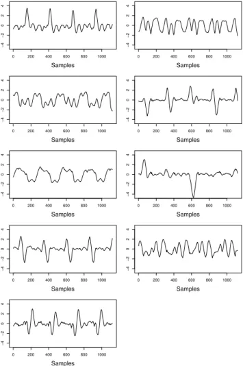
Fig. 2. The examples of the ICA basis functions which are obtained from a single fan: The signals are estimated to be statistically independent by the fastICA method, and they seem to share the characteristics partially.
considered to apply this method to a single-channel mixture using the spectrogram. Such the application is proposed by Casey and Westner [8]. The Casey and Westner develops the powerful framework for decomposition of the audio data and it is possible to reconstruct the meaningful data from the subspace components. In our case, we assume that a number of time series composed of the ICA basis functions are separated into the subspaces by the clustering methods based on as follows.
In order to estimate the subspace, it is necessary to measure the similarities between the ICA basis functions correctly, and to apply the exact clustering method. This time, we focus on just the similarity. For each pair of the ICA basis functions which are time series, their similarities are measured by the following two indicators:
1) Pearson product-moment correlation coefficient:
Cor(x, y) =
∑
i
(xi−x¯)(yi−y¯)
√ ∑
i
(xi−x¯)2 √
∑
i
(yi−y¯)2
. (9)
Where x and y are the input time series, x¯ and y¯ are each average value. This indicator represents the temporal similarities between the ICA basis functions. Using this indicator, it is needless to take into account the ambiguity
of their signs, so that the correlation coefficients has a value of positive and negative. Thus, if the absolute value is taken after the calculations, it would be possible to measure the similarities of each others even for a reverse phase signal.
2) Jensen-Shannon divergence:
DJ S(q||p) = 1
2(DKL(p||q) +DKL(q||p)). (10)
DKL(q||p) = ∫
p(x) log (
p(x)
q(x) )
dx. (11)
WhereDKLis the Kullback-Leibler divergence. The Jensen-Shannon divergence is the symmetrization of theDKL, and this is used in [8]. This indicator represents the probabilistic similarities between the probability distribution of the ICA basis functions, and the probability distribution is estimated by the kernel function that “Gaussian kernel” is used. How-ever, it is necessary to take the absolute in this case.
Using the similarities in the above two methods, these are applied to the group-average clustering method which is one of the popular hierarchical clustering methods [9]. This method can evaluate cluster quality based on all similarities. Also, it is known as being able to avoid difficult problems of the single-link and complete-link criteria, which identify cluster similarity with the similarity of a single pair of components.
C. Feature Extraction
After the clustering of the ICA basis functions by these procedures, they are integrated by taking their averages, and the integrated signals can be regarded as signals with the characteristic of each subspace. However, it is remaining am-biguity of the order which is called a permutation problem. As this countermeasure, we take a sort method based on the magnitude of the variance so that the signals which is integrated into the subspace are able to divide into moderate and intense signal in perspective.
Subsequently, we perform the feature extraction for each of the integrated signals. We employ the five measures as features extracted from the integrated signals. There are two main types of features. One is the three of the frequency domain features that are focused on a periodicity of signals, and the other is the two of the non-Gaussianity features that are focused on the frequency distribution of ones. The former intends that the power spectrum of the integrated signals has various frequency ranges and powers, the latter intends that the frequency distributions of the ones are statistically different. The details of those two types of features are as follows:
1) Frequency Domain Features: After conversion to the signal power spectral density by using FFT, this features are given by
H =∑
i
Fi ∑
iFi log
( ∑ iFi
Fi )
(12)
0.5m 0.
5m
0. 5m The fans
The radar
Pattern A Pattern B
0.5m
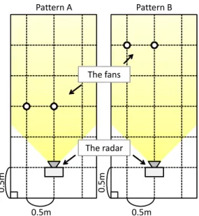
Fig. 3. The Arrangement of the radar and the electric fans: The left shows the pattern A that the radar and the fans are arranged at intervals of 1.0 meter. The right shows the pattern B that the radar and the fans are arranged at intervals of 2.0 meter. The two fans are located in each pattern, EF-D945W is left and F-LN5 is right.
2) Non-Gaussianity Features:
skewness(x) = E[x
3
]
E[(x−x¯)2]32. (13)
kurtosis(x) =E[x
4
]
E[x2]−3. (14)
Where skewness is a measure of the asymmetry of the density function, and kurtosisis a measure of whether the inputs are peaked or flat relative to the Gaussian distribution. After the features are calculated, their values are used in a classification procedure.
IV. EXPERIMENT
A. Experimental Conditions
We used the 24-GHz continuous-wave (CW) microwave Doppler radar (IPS-154) that was manufactured by InnoSent Co., Ltd. Regarding the electric fans, we used two different types. The one was F-LN5 manufactured by Toshiba Co., Ltd, which had a period of about 18 s. The other was EF-D945W manufactured by TWINBIRD Co., Ltd, which had a period of about 10 s. In the experiment, the radar was placed in the room shown by Fig3. Then, because of an effect of distance between the radar and the fans, the experiment was carried out in the two patterns A and B. The height of the fans and the radar were approximately equal to about 0.8 meter. In these conditions, the data were acquired.
B. Data Acquisition and Analysis Process
A number of label data we acquired was 3×2. The breakdown of this first term “3” showed the state that either of the fans was moving and the state that the both fans were moving. Recalling the parameters about the distance with patterns A and B, the total was equal to 6. Each data were sampled at 500Hz and acquired in 9 m. It was configured that the FFT window function was “Hamming
window”, and this size was configured to 2048 samples. Also, a window was slided by 20 samples. The threshold of the cumulative contribution ratio of the SVD was set up at 0.8. The clustering number of ward’s method was configured to 2.
These acquired data was recognized by theSupport Vector Machine(SVM) which was Multi-class classifier. In this case, we used the soft-margin SVM so that the features of the label data were mixed with each other, and a soft-margin parameter C was configured to 1. The maximization of the margin was achieved by using the positive definite kernel function which was “Gaussian kernel”. The identification window size for applying the SVM was composed of 40 s, and it was overlapping by a second.
C. Result
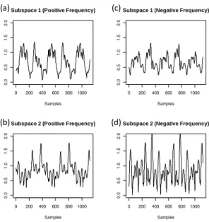
1) Integrated the ICA Basis Functions: Fig4. shows the result of integrating the ICA basis functions into the subspace 1 and 2 is obtained from the mixed-signal during about the 40 s. On the other hand, Fig5. and Fig6. shows the results are obtained from a single fan on similar condition. Fig5. is compatible with F-LN5 which is arranged in a linear direction of the radar, and Fig6. corresponds with EF-D945W. Looking at these different subspaces, they are divided into the slow and fast vibration waveforms. Paying attention to the difference of positive and negative frequency, they are similar in perspective, but its temporal positions of the peaks are different. This is considered that it is caused by the oscillation components of the fans.
2) Recognition by the SVM: The purpose of this study is to recognize the number of oscillating fans. This time, we do not take account into the case that fans are not present. So it is easy to recognize this case, because its amplitude is very different in comparison with others. It is necessary to consider about the parameters which are related to distances and indicators about the clustering process. For simplicity,
Subspace 1 (Positive Frequency)
Samples 0 200 400 600 800 1000
0
.0
0
.5
1
.0
1
.5
2
.0
Subspace 2 (Positive Frequency)
Samples 0 200 400 600 800 1000
0
.0
0
.5
1
.0
1
.5
2
.0
Subspace 1 (Negative Frequency)
Samples 0 200 400 600 800 1000
0
.0
0
.5
1
.0
1
.5
2
.0
Subspace 2 (Negative Frequency)
Samples 0 200 400 600 800 1000
0
.0
0
.5
1
.0
1
.5
2
.0
(a) (c)
(d) (b)
Fig. 5. The single signal (by F-LN5 with a period of about 18 s) is integrated into each subspace. The meaning of the symbols is the same as Fig. 4.
Subspace 1 (Positive Frequency)
Samples 0 200 400 600 800 1000
0
.0
0
.5
1
.0
1
.5
2
.0
Subspace 2 (Positive Frequency)
Samples 0 200 400 600 800 1000
0
.0
0
.5
1
.0
1
.5
2
.0
Subspace 1 (Negative Frequency)
Samples 0 200 400 600 800 1000
0
.0
0
.5
1
.0
1
.5
2
.0
Subspace 2 (Negative Frequency)
Samples 0 200 400 600 800 1000
0
.0
0
.5
1
.0
1
.5
2
.0
(a) (c)
(d) (b)
Fig. 6. The single signal (by EF-D945W with a period of about 10 s) is integrated into each subspace. The meaning the of symbols is the same as Fig. 4.
we define the label name of the data, the fan (F-LN5) is referred to as the “F1” and the other fan (EF-D945W) is referred to as the “F2”, also the two fans are referred to as the “MIX”. Now, the SVM classifier is trained by using the “MIX” data as the “two fans” and the binded data which are composed of “F1” and “F2” data as “a single fan”. Also, the training data are only using the pattern B to compare the pattern A. As for the test data for the recognition, it is including all the data. The results of the recognition using the “correlation” for clustering the ICA basis functions is described in TABLE I, and the result of recognition using the “Jensen-Shannon divergence” is described in TABLE II. The values of the results represent the precisions, that is expressed as a percentage. The left side rows indicates the training data, and the upper side columns indicates the test data. As explained in section 2, the microwave
Doppler radar outputs the signals which are proportional to the reflection and distance. The training data which are used by the SVM are obtained in the context of just 2.0 meter distance between the radar and the fans. So it is difficult to recognize the test data by using the training data in the way that their reflection and distance are different as a rule. The accuracies of “correlation” and “Jensen-Shannon divergence” are described in TABLE III. The accuracy indicates that how close a measured value is to the actual value.
TABLE I
THERECOGNITIONPRECISION(%)USED“CORRELATION”
F1(A) F2(A) MIX(A) F1(B) F2(B) MIX(B)
“A single fan” 95
.7 91.4 25.7 100.0 84.3 17.1
“Two fans” 4
.3 8.6 74.3 0.0 15.7 82.9 TABLE II
THERECOGNITIONPRECISION(%)USED“JENSEN-SHANNON DIVERGENCE”
F1(A) F2(A) MIX(A) F1(B) F2(B) MIX(B)
“A single fan” 100
.0 85.7 4.3 100.0 95.7 0.0
“Two fans” 0
.0 14.3 95.7 0.0 4.3 100.0 TABLE III
THEACCURACY(%)
The indicators Accuracy
Correlation 88
.1
Jensen-Shannon divergence 96
.2
V. CONCLUSION
In this paper, we proposed a method based on ICA using the Doppler signals to detect the number of the oscillating fans, as a basic research for applying the human sensing data. And the method is applied to the Doppler signals which are generated by the one or two electric oscillating fans. The output signals which are decomposed by the STFT are applied to ICA, and the ICA basis functions are obtained. Subsequently, the subspaces are extracted from the ICA basis functions, and the five features are calculated by each of them. In this process, we compare the two indicators which are used for calculating similarities between the ICA basis functions and the effects of the distance between two different points. The results are obtained by the SVM. In conclusion, the minimum precision for the mixture signal which belongs to the test data is 95.7% in case of using the “Jensen-Shannon divergence”. The accuracies of the two indicators shows that the probabilistic similarities “Jensen-Shannon divergence” are superior to the temporal similarities “correlation” between the ICA basis functions.
REFERENCES
[1] C. Li, J. Cummings, J. Lam, E. Graves, and W. Wu, “Radar remote monitoring of vital signs,”IEEE Microw. Mag., vol. 10, no. 1, pp. 47– 56, February, 2009.
[2] A. D. Droitcour, O. Boric-Lubecke, and J. Lin, “A microwave radio for Doppler radar sensing of vital signs,”IEEE MTT-S Int. Microwave Symp. Dig., vol. 1, pp. 157–178, 2001.
[3] Yanming Xiao, Changzhi Li and Jenshan Lin, “A Portable Noncontact Heartbeat and Respiration Monitoring System Using 5-GHz Radar,”
Sensors Journal, IEEE, vol. 7, no. 7, pp. 1042–1043, July, 2007. [4] K.-W. Gurgel and T. Schlick, “Remarks on Signfal Processing in HF
Radars Using FMCW Modulation,”Proc. of the International Radar Symposium IRS’2009, Hamburg, Germany, Proceedings pp. 63–67, September, 2009.
[5] Mori. T and Sato. T, “Influence of relative position and pose between sensor and human on respiration measurement with microwave Doppler sensor,”Networked Sensing Systems (INSS), Seventh International Con-ference, pp. 97–100, June, 2010.
[6] A. Hyvarinen and E. Oja, “A Fast Fixed-Point Algorithm for Inde-pendent Component Analysis,”Neural Computation, vol. 9, no. 7, pp. 1483–1492, October, 1997.
[7] A. Hyvarinen and P. Hoyer, “Independent subspace analysis shows emergence of phase and shift invariant features from natural images,”
Proc. Int. Joint Conf. on Neural Networks, vol. 2, pp. 1059–1064, July, 1999.
[8] W. Day and H. Edelsbrunner, “Efficient algorithms for agglomerative hierarchical clustering methods,”Journal of Classification, vol. 1, no. 1, pp. 7–24, 1984.
[9] M. A. Casey and A.Westner, “Separation of mixed audio sources by independent subspace analysis,”Proc. Int. Comp. Music Conf., Berlin, Germany, pp. 154–161, May, 1997.