A Work Project, presented as part of the requirements for the Award of a Master Degree in Economics from the NOVA - School of Business and Economics.
Catastrophic health care expenditures in Portugal and
its drivers
Francisca Miguel Leitao Silva Pinhao
#3119
A Project carried out on the Master in Economics Program, under the supervision of: Prof. Pedro Pita Barros
Titulo
Abstract
This work assesses levels, drivers and policy implications of catastrophic health ex-penditures (CHE) in Portugal in the year of 2015. Moreover by following the same methodological approach as studies for previous years, it allows for comparison and assessment of evolution. CHE incidence is calculated. Possible determinants of CHE are estimated through a logistic model. A simulation of additional coverage of pharma-ceutical is presented. Main findings point to a decrease in the level of CHE from 2010 to 2015, identify elderly as the most exposed group and estimate a decrease in CHE of up to 1pp as consequence of a higher coverage of pharmaceuticals.
1
Introduction
Studies on health economics provide important insights in terms of policy making. The topic itself is very sensitive and deserves special attention. Countries have different methods of financing health sector. The Portuguese Constitution (1976) states the right to universal and comprehensive health services approximately free of charge. However, in 2013 Portugal registered a share of out-of-pocket spending of 28% (OECD, 2015), well above the average across the OECD countries (19%). The economic reasoning behind out-of-pocket payments is closely linked to the concept of efficiency and aims at reducing overconsumption due to moral hazard. However, this can lead individuals having to pay large proportions of their available income resulting in pushing them into poverty. A study for the USA (Merlis, 2002) shows that when a head of households is an older person, a person with disability or is unemployed those households are more likely to be affected when compared to others. For the case of Portugal there are evidence of this being a sizeable issue. Kronenberg and Barros (2014) identify the most vulnerable groups and suggest exemption for some of them, as a way of mitigate the tendency for those incurring in catastrophic health care expenditures. Most recent works as Borges (2013) show that even with enlarged economic exemptions increases in user charges have a harmful effect on the percentage of people incurring in catastrophic health care expenditures.
The objective of this work is to continue the research that has been done on the topic for Portugal, resorting the same data source although for more recent periods. In the light of recent economic crisis, analyzing data from 2015 has increased interest. A comparison is established not only with the previous studies above mentioned but also with research on income inequality and impoverishment as a consequence of the crisis, namely Rodrigues et al. (2016). Lastly, a simulation and scenarios analysis are also done regarding pharmaceuticals’ coverage and the effects of hypothetical increases of it on the percentage of people incurring in catastrophic health care expenditures.
concept and ways of measuring catastrophic health care expenditures. Section 3 presents the data and methodology. Results are reported in Section 4. Section 5 provides an analysis on the impact of pharmaceuticals’ coverage on CHE. A reflection on health care expenditures during crisis aftermath is presented on Section 6. Section 7 concludes.
2
Literature Review
Berki (1986) has firstly introduced the concept of catastrophic expenditure defining it as one which represents a large part of household budget and therefore affects its ability to keep customary standard of living. Russel (1996) pointed out the concern about the opportunity cost of health care spending. This view has been reinforced by later studies which have also been providing different measures of catastrophic expenditures.
Wagstaff and Doorslaer (2003) have firstly applied two different approaches to the concept of catastrophic health care expenditures (CHE). The first one sets the threshold in terms of proportionality of income by considering the OOP payments as a proportion of the income and usually setting the thresholds between 2.5% and 15%. The fact that in this approach same thresholds are used regardless of the financial condition of the household raises issues related to the greater probability of richer households exceeding the threshold with much less severe consequences than those for the poorest households. Authors’ second approach introduces the concept of “capacity to pay” and defines it as the total expenditures except the subsistence need. By doing this the authors are able to estimate incidence of CHE after allowing deductions for food expenditure. Health expenditure is therefore considered as a fraction of household income subtracting food expenditure.
Xu et al. (2003) suggests another approach for measuring household’s capacity to pay for health care by subtracting the food expenditure of the median household from households’ income. Households that spend more than 40% of their capacity to pay on health care are considered to incur in CHE.
pay-ments exceed a threshold of the household’s capacity to pay, which in the case of this study has taken several values between 10% and 40%.
3
Data and Methodology
3.1
Survey Description
Data comes from a national representative household survey, the Portuguese Household Budget Survey – IDEF - Inquérito às Despesas das Famílias – which included 11398 house-holds interviewed between March of 2015 and March of 2016. The survey was carried out by Statistics of Portugal (INE), the official body in charge of production of data on the country, and represents the most recent edition of data series on household budgets, following the work that has been done since the 60s.
3.2
Dependent Variable
Catastrophic health care expenditure (CHE) occurs when a household’s total out-of-pocket (OOP) healthcare payments equal or exceed a certain threshold of their capacity to pay for non-subsistence spending. The term catastrophic is related to what happens to the opportu-nity cost of health care expenditure when households are not able to spend a given fraction of their resources on other goods and services besides it, due to excessive OOP payments.
For comparison purposes the most common threshold in the literature was used, following the WHO definition and setting it as 40%. Following Wagstaff and Doorslaer (2003) and Xu et al. (2003) CHE is defined with respect to capacity to pay. This last concept corresponds to the difference between total expenditures and the subsistence spending of a household. In this study subsistence needs were computed as the median food expenditure of the households, in line with Xu et al. (2005). Notwithstanding Evetovits et al. (2012) approach was also tested, considering an extended basket including expenses other than food, namely clothing and utility bills. Similarly, and regardless of the adoption of WHO definition of CHE, others
thresholds were tested, namely 10%, 20% and 30%.
Analytically and following Borges (2013), let Y be OOP, x the total household expendi-ture, f(x) the household subsistence spending and z the defined threshold. A household i will therefore be said to incur in CHE if: Yi
xi−f (xi ) ≥ z. As it is easily perceived, the condition
Yi >0 is imposed, meaning that only OOP payments greater than zero can be considered in
the assessment of CHE. It raises a limitation of CHE highlighted by Wagstaff and Doorslaer (2003): the potential exclusion of households in a situation of such poverty that prevent them from having any access to medical care.
3.3
Independent Variables
Poverty Line: In order to be able to relate impoverishment and health care expenditures a poverty line has been computed. OECD approach has been followed as it is easily found in previous related research as in Kronenberg and Barros (2014) and Borges (2013). Therefore, poverty line is defined as 60% of median income. Household income is considered after adjustment using the equivalence square root method. From the poverty line it is therefore derived the concept of poverty rate, computed as the fraction of people under the poverty line in the total of individuals of the different groups.
Set of explanatory variables: the choice of determinants of CHE was made based on the availability of data and in line with the literature on the topic. An initial assessment on the individual significance was made by running logistic regressions for each one of them, allowing to use the statistically significant ones together in the subsequent analyses.
3.4
Model
The independent variable above characterized, the incurrence of CHE, takes a binary form, assuming the value 1 if the household incurs in CHE and the value 0 otherwise. Following Kronenberg and Barros (2014) and the general literature on the topic, a logistic regression has been chosen to model the problem. Hence, the probability p of falling into CHE is:
pi = Pr (yi = 1| x) = F (x0iβ) = ex0iβ
1+ex0iβ. F (.) is the logistic cumulative distribution function ensuring that 0≤p≤1. The coefficients are log-odds and are interpreted as the variation in the logit for a unit variation in the explanatory variable. In order to make this interpretation more complete and keeping in mind the interest of preserving similarities with previous studies in order to seek their comparability, odds-ratio are reported, following Kronenberg and Barros (2014) and Borges (2013). Odds-ratio provides the ratio of the odds of an event occurring in one group relatively to the odds of another event. When odds-ratio takes the value 1 we face two regressors with the same probability of causing an event, y. If it assumes a value below 1 (but strictly positive), there is a regressor x with lower probability of causing y than the baseline. In an opposite way, when odds-ratio is above 1, the regressor x is more likely to cause y than the one which it is being compared. Marginal effects are computed as AMEs (average marginal effects) due to the fact of being observation specific. Hence they calculate the marginal effect of a regressor for each household in the sample and subsequently present their average.
4
Results
4.1
Incidence of CHE
Tables 1, 2 and 3 present the proportion of Portuguese households incurring in CHE in 2015 by region and income quintile and different measures of catastrophe are computed. In (1) subsistence needs are considered as food expenditures accordingly to WHO definition and in line with Borges (2013) while in (2) the concept becomes broader, considering an extended
Table 1: CHE proportion per income group CHE40 CHE30 CHE20 CHE10 1st quintile 0.05085 0.10748 0.22117 0.45597 2nd quintile 0.01462 0.04219 0.12573 0.34962 3rd quintile 0.00044 0.01237 0.06452 0.24790 4th quintile 0.00094 0.00897 0.04627 0.22993 5th quintile 0.00091 0.00272 0.02132 0.16697 Overall (1) 0.01430 0.03632 0.09888 0.29444 Overall (2) 0.04685 0.07940 0.15345 0.35322
Table 2: CHE proportion per household type
CHE40 CHE30 CHE20 CHE10
1 adult 0.01044 0.02372 0.05598 0.19734 1 elderly 0.05670 0.12107 0.25134 0.52261 2+ adults 0.00329 0.01646 0.04937 0.22379 2+ adults/elderly 0.02386 0.06339 0.17984 0.47187 1 adult + children 0.00000 0.00378 0.04537 0.18904 2+ adults + 1 child 0.00202 0.00605 0.03530 0.17751 2+ adults + 2+ children 0.00000 0.00251 0.02261 0.13379
basket including expenditures in food, clothing and utilities. The remaining analysis for region, income quintiles and household type consider the method in (1).
The results presented for incidence of CHE by household type reveal large disparities. Households including elderlies are clearly the most affected ones, especially one-person house-holds. In fact by relaxing the concept of CHE and focusing on the first column for a CHE level of 10%, one concludes that more than half of the one-elderly households are exposed to
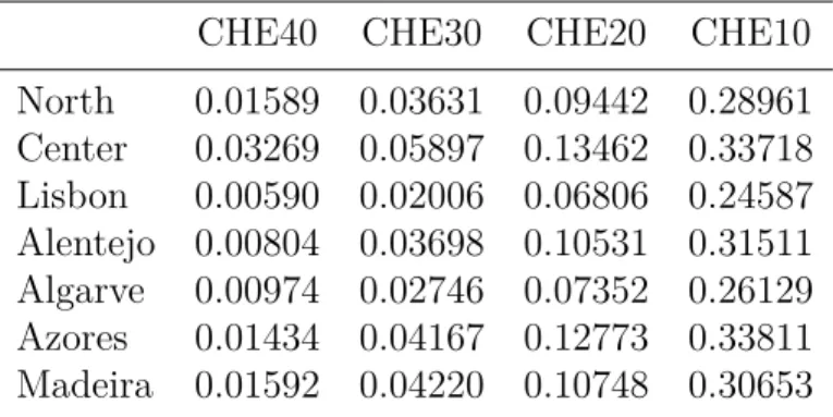
Table 3: CHE proportion per Region CHE40 CHE30 CHE20 CHE10 North 0.01589 0.03631 0.09442 0.28961 Center 0.03269 0.05897 0.13462 0.33718 Lisbon 0.00590 0.02006 0.06806 0.24587 Alentejo 0.00804 0.03698 0.10531 0.31511 Algarve 0.00974 0.02746 0.07352 0.26129 Azores 0.01434 0.04167 0.12773 0.33811 Madeira 0.01592 0.04220 0.10748 0.30653
it. In line with this, the second most affect group is the one composed by households with two or more adults and at least one elderly.
Table 4 allows for a comparison between the values for 2015 and those resulting from the three previous Portuguese Household Budget Survey held in 2000, 2005 and 2010, using data from Borges (2013).
Borges (2013) found results for catastrophe in Portugal in 2000, 2005 and 2010 of respec-tively 5.005%, 3.177% and 2.439%. The result obtained for 2015 (1.43%) reveals a variation of -1.009pp for the last 5 years, slightly higher than the one between 2005 and 2010 (-0.738pp). Xu et al. (2007) performed an incidence analysis of CHE in 89 countries and found a median level of 1.47%. Therefore, in the time frame for which there are available data, that is, between 2000 and 2015, the last year was the first Portugal performed above the median value, although only slightly.
At a regional level, Center registers more percentage of CHE, followed by North and Madeira. Lisbon has the lowest values. Borges (2013) has reported Azores and Madeira to be the most affected regions in 2010 closely followed by Center.
Concerning income levels, differences are observed. 1st quintile, corresponding to the poorest one, has the higher percentage of incidence. It then continuously decreases until the second two quintiles that in fact register the same value. This is in line with the literature on the topic (Wagstaff and Doorslaer, 2003). When comparing the income quintiles analysis with Borges (2013) results for 2010 it is clear that the poorest quintile was the one that remained more affected. The other four quintiles have registered variations between 0.59pp and -1.07pp. The first one however has only decreased by 0.47pp. The difference in the pattern of CHE occurrence across income quintiles when compared with Borges (2013) may be due to significant changes in the income distribution itself, therefore affecting the determination of the quintiles. However, more data would be needed in order to conclude about the topic. Comparison on the occurrence of CHE by household type is not possible, since such data is not available from Borges (2013).
Table 4: Comparison between year of analysis and data on previous years (Borges, 2013) 20001 20051 20101 20152 CHE40 5.005% 3.177% 2.439% 1.43% Region North 3.527% 3.011% 2.439% 1.59% Center 6.097% 3.836% 2.485% 3.27% Lisbon 4.990% 2.287% 2.264% 0.59% Alentejo 7.315% 5.350% 2.969% 0.80% Algarve 7.794% 2.749% 1.827% 0.97% Azores 7.331% 2.552% 3.090% 1.43% Madeira 5.832% 3.964% 3.062% 1.59% Income quintile 1st 15.711% 8.519% 5.556% 5.09% 2nd 8.218% 5.558% 2.283% 1.46% 3rd 3.384% 1.930% 1.112% 0.04% 4th 1.417% 0.854% 0.813% 0.09% 5th 0.393% 0.593% 0.681% 0.09%
4.2
Econometric modelling of CHE determinants
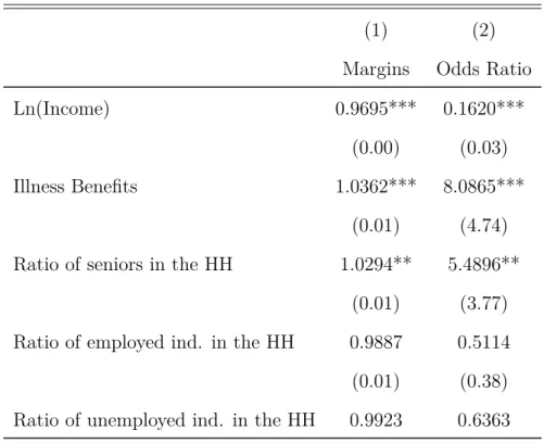
Table 5: Margins and Odds Ratio from logistic regression
(1) (2)
Margins Odds Ratio
Ln(Income) 0.9695*** 0.1620***
(0.00) (0.03)
Illness Benefits 1.0362*** 8.0865***
(0.01) (4.74) Ratio of seniors in the HH 1.0294** 5.4896**
(0.01) (3.77) Ratio of employed ind. in the HH 0.9887 0.5114 (0.01) (0.38) Ratio of unemployed ind. in the HH 0.9923 0.6363
1Source: Borges (2013). 2Own calculations.
(0.01) (0.42) EDUC 4th Grade 0.9912** 0.6295** (0.00) (0.12) 6th Grade 0.9823*** 0.2911** (0.01) (0.16) 9th Grade 0.9905 0.6037 (0.01) (0.27) High School 0.9774*** 0.1185** (0.01) (0.13) Higher Education 0.9790*** 0.1759 (0.01) (0.19) NUTS Center 1.0120** 1.6668** (0.01) (0.42) Lisbon 0.9877*** 0.4007*** (0.00) (0.14) Alentejo 0.9874*** 0.3896** (0.00) (0.15) Algarve 0.9906* 0.5335* (0.01) (0.20) Azores 0.9974 0.8682 (0.01) (0.28) Madeira 1.0055 1.2953 (0.01) (0.40) N 8259 8259
Exponentiated coefficients * p<0.10, ** p<0.05, *** p<0.01
The log-transformed income variable is statistically significant at 1% level. Its odds-ratio is smaller than 1, evidencing that a higher level of income leads to a lower probability of facing CHE, which goes in line with economic intuition.
The fraction of senior people on the household seniorratiois also statistically significant
at 1% level and presents an odds-ratio above 1, as expected. Households composed by elderly people are more likely to incur in CHE.
The ratios of employed, unemployed and unable to work people on the household size are all not significant, in contrast with previous literature as Borges (2013) and Kronenberg and Barros (2014) who found significant results for at least one of them.
Regarding age of the head of household none of the dummy variables turned out to be significant, differently from what Borges (2013) found.
Except for 9th grade, all the other variables related to education of the head of household are significant at a 5% level. All the odds-ratio are lower than 1, leading to the interpretation that a degree of education decreases the likelihood of incurring in CHE, when compared to none.
When comparing these results with Borges (2013) for the years of 2000, 2005 and 2010 one finds the same effect of education of the head of household, meaning significance and magnitude of the odds-ratio. Similar thing happens for the ratio of seniors in the household, even though it only holds for 2010 and current results for 2015 present a higher odds-ratio.
5
The impact of pharmaceuticals’ coverage on CHE
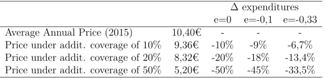
Pharmaceuticals are the biggest source of heath spending, having accounted for more than 71% of the expenditure in health care in 2015. To assess the effects of an increase in coverage
of pharmaceuticals on CHE a simulation is performed under two different scenarios. In the first one it is assumed a price elasticity of demand for the consumption of pharmaceuticals of 0. In the second one, and based on the literature in the topic, lower and upper bounds for price elasticity are used. Accordingly to Ringel et al. (2002) I have set the bounds as -0,1 and -0,33. From the natural interpretation of elasticities, comes that a reduction of 1% in the pharmaceuticals’ price leads to a 0,1% or 0,33% increase in their consumption. The Portuguese Authority of Medicines and Health Products, Infarmed (Infarmed, 2015), provides data on the average annual prices of pharmaceuticals. Following the 2 scenarios above mentioned I have tested for 3 hypothetical levels of additional coverage. Table 6 presents the expected variation on pharmaceuticals’ expenditures.
Table 6: Estimates of variation in pharmaceuticals expenditures ∆ expenditures e=0 e=-0,1 e=-0,33
Average Annual Price (2015) 10,40€ - -
-Price under addit. coverage of 10% 9,36€ -10% -9% -6,7% Price under addit. coverage of 20% 8,32€ -20% -18% -13,4% Price under addit. coverage of 50% 5,20€ -50% -45% -33,5%
From this reduction on pharmaceuticals’ expenditures – and consequently in health ex-penditures – two scenarios are possible: households can allocate the disposable income to any other good or service, keeping their total expenditures level constant; or they can decide not to allocate the surplus, causing the total expenditures to decrease. The impacts of both alternatives on CHE are detailed on tables 7 and 8.
Table 7: Estimates for occurrence of CHE under additional coverage – constant level of household expenditures
e=0 e=-0.1 e=-0.33 Reference 10% 0.01149 0.01193 0.01246
0.01430 20% 0.00956 0.01009 0.01079
Table 8: Estimates for occurrence of CHE under additional coverage - adjusted household expenditures
e=0 e=-0.1 e=-0.33 Reference 10% 0.01281 0.01290 0.01325
0.01430 20% 0.01097 0.01132 0.01202
50% 0.00649 0.00728 0.00921
6
Health care expenditures during crisis aftermath
The recent past of the country, which faced an intense economic crisis, was particularly demanding. Rodrigues et al. (2016) show a decrease in income of more than 12% between 2009 and 2014. Moreover, they report that between 2009 and 2012 69% of the individuals suffered from that income decrease. In the same study the authors focus on understanding which groups were most affected. In this section a comparison is made between Rodrigues et al. (2016) findings and the sample being analyzed.
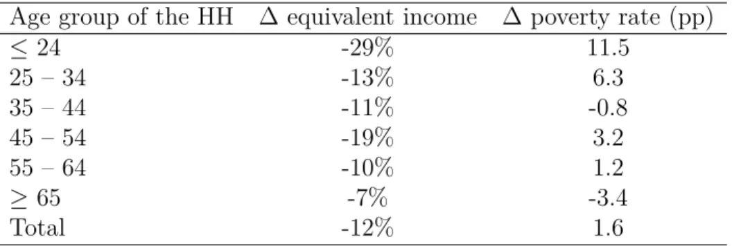
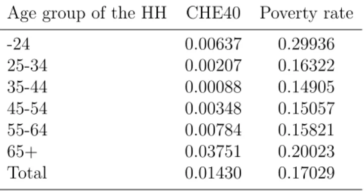
Table 9: Variation of income and poverty rates by age group of the head of household between 2009 and 2014
Age group of the HH ∆ equivalent income ∆ poverty rate (pp)
≤ 24 -29% 11.5 25 – 34 -13% 6.3 35 – 44 -11% -0.8 45 – 54 -19% 3.2 55 – 64 -10% 1.2 ≥ 65 -7% -3.4 Total -12% 1.6 Source: Rodrigues et al (2016)
Rodrigues et al. (2016) findings show that households which individual of reference is a senior (last age group) were the least affected by the decrease in income. Both the variation in equivalent income and the poverty rate show the best evolution in the time frame considered. This data contrasts with the current analysis, as we can see that the elderly age group still reveals the higher percentage of CHE in 2015. However, another variables need to be taken into account such as the natural increased likelihood of older people to become sick and
Table 10: Percentage of occurrence of CHE and poverty rate for 2015 Age group of the HH CHE40 Poverty rate
-24 0.00637 0.29936 25-34 0.00207 0.16322 35-44 0.00088 0.14905 45-54 0.00348 0.15057 55-64 0.00784 0.15821 65+ 0.03751 0.20023 Total 0.01430 0.17029
therefore to incur in higher health care expenditures.
On the other hand, when analyzing the poverty rate for 2015 it becomes easier to relate with the referred literature. In fact the youngest age group reveals the third highest percent-age of CHE in the sample. The authors emphasize the low level of income of this percent-age group, a circumstance that persists in the year of this analysis. It is intuitively concluded that this condition turns this population group into a vulnerable one, when it comes to CHE.
7
Conclusion
This work analyses data from 2015 on CHE allowing it to be compared with previous years. Regarding the occurrence of CHE it registers a decrease from 2.439% to 1.43%, evidencing an improvement of the overall condition of the households related to CHE. Occurrence by household type shows a lot of heterogeneity across categories with clear evidence of the unfavourable condition of the elderly. The two household groups containing people above 65 years old register the higher values for CHE occurrence. The analysis by income quintiles reveals a predominance of a higher percentage of CHE at lower income levels. Occurrence of CHE by income quintiles show a different pattern from the last years, suggesting a change in income distribution which couldn’t be adequately investigated in this context.
Concerning the determinants of CHE only income, receiving illness benefits, fraction of people above 65 years old on the household, region and education of the head of household are statistically significant in the analysis.
The high poverty rate on both the lowest and the highest age groups should get attention from policy makers. The latest situation, of the highest age group, when put together with the currently percentage of CHE, confirms that the elderly are a group that needs protection from against catastrophe.
The simulation on additional coverage of pharmaceuticals has revealed the potential de-crease in CHE occurrence. For an additional 10% coverage level, the estimates point to a reduction between 0.105pp and 0.281pp. For the scenario of 20% additional coverage those values vary between 0.228pp and 0.474pp. Lastly, an additional 50% coverage would result in a decrease in the percentage of CHE between 0.509 and 1.00 pp. A policy with similar results to those of the additional coverage may be to ensure the decrease of pharmaceuticals’ price through, for example, promotion of generics.
References
OECD. How does health spending in portugal compare? 2015.
Mark Merlis. Family out-of-pocket spending for health services: a continuing source of
finan-cial insecurity. Commonwealth Fund New York (NY), 2002.
Christoph Kronenberg and Pedro Pita Barros. Catastrophic healthcare expenditure–drivers and protection: the portuguese case. Health Policy, 115(1):44–51, 2014.
Ana Rita Galrinho Borges. Catastrophic health care expenditures in Portugal between
2000-2010: Assessing impoverishment, determinants and policy implications. PhD thesis,
NSBE-UNL, 2013.
C FARINHA Rodrigues, R Figueiras, and V Junqueira. Desigualdade do rendimento e po-breza em portugal: As consequências sociais do programa de ajustamento. Fundação
Francisco Manuel dos Santos, page 92, 2016.
SE Berki. A look at catastrophic medical expenses and the poor. Health affairs, 5(4):138–145, 1986.
Adam Wagstaff and Eddy van Doorslaer. Catastrophe and impoverishment in paying for health care: with applications to vietnam 1993–1998. Health economics, 12(11):921–933, 2003.
Ke Xu, David B Evans, Kei Kawabata, Riadh Zeramdini, Jan Klavus, and Christopher JL Murray. Household catastrophic health expenditure: a multicountry analysis. The lancet, 362(9378):111–117, 2003.
Ke Xu, World Health Organization, et al. Distribution of health payments and catastrophic expenditures methodology. 2005.
T Evetovits, P Gaal, S Szigeti, F Lindeisz, and J Habicht. Informing decision makers: Analysis of financial protection over time in the context of policy change. In European
Conference on Health Economics, 2012.
Ke Xu, David B Evans, Guido Carrin, Ana Mylena Aguilar-Rivera, Philip Musgrove, and Timothy Evans. Protecting households from catastrophic health spending. Health affairs, 26(4):972–983, 2007.
Jeanne S Ringel, Susan D Hosek, Ben A Vollaard, and Sergej Mahnovski. The elasticity of demand for health care. a review of the literature and its application to the military health system. Technical report, RAND NATIONAL DEFENSE RESEARCH INST SANTA MONICA CA, 2002.
8
Annex
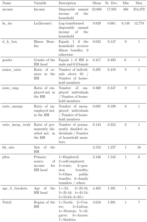
Table 11: Descriptive statistics
Name Variable Description Mean St. Dev. Min Max
income Income Disposable annual
income of the household
23,088 17,935 468 354,270
ln_inc Ln(Income) Log-transformed
disposable annual income of the household
9.829 0.661 6.148 12.778
d_h_ben Illness
Bene-fits Equals 1 if thehousehold receives illness benefits; 0 otherwise
0.022 0.147 0 1
gender Gender of the
HH head Equals 1 if HH ismale and 0 if female 0.417 0.493 0. 1 senior_ratio Ratio of
se-niors in the HH Number of individ-uals above 65 / Number of house-hold members 0.295 0.418 0 1
ratio_emp Ratio of
em-ployed ind. in the HH Number of em-ployed individuals / Number of house-hold members 0.369 0.347 0 1
ratio_unemp Ratio of
un-employed ind. in the HH Number of unem-ployed individuals / Number of house-hold members 0.085 0.199 0 1
ratio_incap_work Ratio of per-manently dis-abled ind. in the HH
Number of perma-nently disabled in-dividuals / Number of household mem-bers
0.144 0.224 0 1
hh_size Size of the
HH 2.552 1.237 1 16 pfrm Primary source of income for HH head 1=Employed; 2=self-employed; 3=rents; 4=pen-sion benefits; 5=Other public benefits; 6=family transfers / others 2.448 1.542 1 6
age_b_brackets Age of the
HH head 1=-24;3=35-44; 4=45-54;2=25-34; 5=55-64; 6=65+
4.403 1.391 1 6
Nuts2 Region of the
HH 1=North; 2=Cen-ter; 3=Lisbon; 4=Alentejo; 5=Al-garve; 6=Azores; 7=Madeira