AdS Black Holes from
Localized Boundary
Sources
João Pedro Alves da Silva
Mestrado em Física
Departamento de Física e Astronomia da Universidade do Porto 2015
Orientador
Miguel Sousa Costa, Professor Associado, Faculdade de Ciências da
Universidade do Porto
Co-orientador
Jorge Eduardo Santos, Lecturer in Theoretical Physics, University of
Cambridge
Todas as correções determinadas pelo júri, e só essas, foram efetuadas.
O Presidente do Júri,
Acknowledgements
I’m very thankful for these 5 years in Porto, in particular for the past months where I’ve started to engage in research. I’d like to show my gratitude to Jorge Santos, for all his time and guidance. My time in Cambridge was very instruc-tive. I’d also like to thank Miguel Costa for teaching me a lot of subjects. More generally, I’m grateful for all the friends and colleagues in FCUP.
I acknowledge the Gulbenkian Foundation for the significant financial sup-port provided through Programa de Est´ımulo `a Investigac¸˜ao 2014.
Abstract
We study a massive scalar field in a spacetime with a negative cosmologi-cal constant. We impose as boundary conditions that, near the conformal boundary, spacetime is AdS and the scalar field behaves as a localized de-fect. For the values of the field strength B examined, we provide evidence
that no Schwarzschild AdS black hole is formed. This is to be contrasted with the findings in Hovering Black Holes from Charged Defects, [Class. Quant. Grav., vol. 32, no. 10] by Horowitz, Iqbal, Santos and Way, where the authors considered an analogous setup, but with a maxwell field, instead of a scalar field. They found that, for a large class of profiles for the boundary maxwell field, a Reissner-N¨ordstrom AdS black hole is formed in the bulk.
In this thesis, we also review some topics involved in numerically solving the Einstein equations, namely the deTurck gauge and spectral methods in general relativity. We perform perturbative calculations as a check on our numerical work.
Resumo
Estudamos um campo escalar massivo, num espac¸o-tempo com constante cosmol´ogica negativa. Impomos como condic¸˜ao de fronteira que, perto da fronteira conforme, o espac¸o-tempo ´e AdS e o campo escalar comporta-se como um defeito localizado. Para os valores do coeficiente do campo B
ex-aminados, damos ind´ıcios de que nenhum buraco negro Schwarzschild AdS se forma. Isto deve ser contrastado com as investigac¸˜oes em Hovering Black Holes from Charged Defects, [Class. Quant. Grav., vol. 32, no. 10] por Horowitz, Iqbal, Santos e Way, em que os autores consideraram um cen´ario an´alogo, mas com um campo de maxwell, ao inv´es de um campo escalar. Eles obtiveram que, para uma vasta gama de tipos de campos de maxwell na fronteira, forma-se um buraco negro AdS Reissner-N¨ordstrom no interior do espao-tempo.
Nesta tese, tamb´em explicamos alguns t´opicos envolvidos na resoluc¸˜ao num´erica das equac¸˜oes de Einstein, nomeadamente o calibre de deTurck e m´etodos espectrais em relatividade geral. Fazemos c´alculos perturbativos de maneira a validar os nossos resultados num´ericos.
Contents
1 Introduction 1 2 deTurck Gauge 2
2.1 General Remarks and Definition . . . 2
2.2 Diffeomorphisms . . . 4
2.3 Implementing the deTurck gauge . . . 5
3 Chebyshev Polynomials and Newton’s method 7 3.1 Chebyshev Polynomials . . . 7
3.2 Newton’s method . . . 8
4 Gauge Gravity Duality 10 4.1 Anti-deSitter Space . . . 10
4.2 Anti-deSitter Black Holes . . . 18
4.3 Some comparisons between gravity in AdS and CFT’s . . . 19
5 Hovering Black Holes from Charged Defects 24 6 Setup 25 7 Boundary Conditions 27 7.1 Conformal Boundary . . . 27
7.2 Regularity Condition at x = 0 . . . 27
7.3 IR Horizon: irrelevant profile . . . 27
7.4 IR Horizon: marginal profile . . . 28
8 Bulk Spacetime 30 9 Discussion and Further Work 35 Appendix 35 Appendix A - Perturbative Calculation for ODE’s . . . 35
Appendix B - Perturbative Calculation for PDE’s . . . 39
Appendix C - Weyl Tensor: definition and properties . . . 45
Appendix E - Spectral method: convergence properties . . . 47 Appendix F - Code Display . . . 49
List of Figures
1 Bounded interval seen from the complex plane. . . 7
2 Penrose diagram of Minkowski space. . . 16
3 Diagram of AdS space. . . 17
4 Comparison between Schwarzschild and Schwarzschild-AdS4 black holes in terms of their specific heat. . . 20
5 Poincar´e Patch in angular coordinates. . . 26
6 Maximum of the Contraction of the Weyl Tensor in the IR horizon as a function of B. . . 29
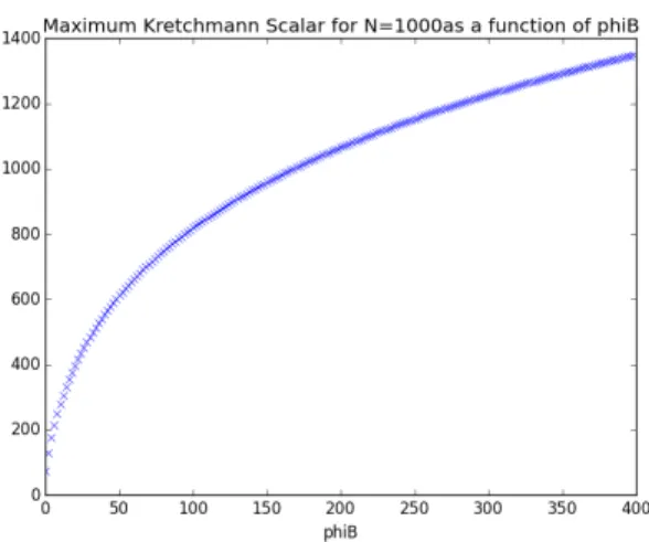
7 Maximum of the Curvature in the IR horizon as a function of B. 29 8 Maximum of the Kretchmann Scalar in the IR horizon as a func-tion of B. . . 30
9 Comparison between numerics and perturbative calculation. Max-imum of the curvature in the IR horizon for a range of values of B. . . 30
10 Maximum of the Curvature in the bulk as a function of B. . . 31
11 Maximum of the Kretchmann scalar in the bulk as a function of B. 31 12 Maximum of the norm of the deTurck vector in the bulk as a function of B. . . 32
13 Maximum of the contraction of the Weyl Tensor in the bulk as a function of B. . . 32
14 Absolute value of the curvature over the Poincar´e patch for B = 2.8. . . 33
15 gttfor x = 0. . . 34
16 Comparison between numerics and perturbative calculation. Max-imum of the Kretchmann Scalar in the bulk spacetime computed for a range of values of B. . . 34
17 Comparison between numerics and perturbative calculation. Kretch-mann Scalar in the IR horizon for B= 0.6. . . 39
18 deTurck norm as a function of grid size. . . 47
19 Kretchmann scalar as a function of grid size. . . 48
21 Newton’s method in python. . . 49
22 Passing expressions from Mathematica to Python. . . 49
23 Writing the differentiation matrices in Python. . . 50
1 Introduction
In [1], the authors solved the Einstein-Maxwell equations with a negative cos-mological constant for a stationary and axisymetric spacetime, imposing that at the conformal boundary the metric is AdS and the maxwell field behaves as a localized source. The main finding was that, for a large class of profiles for the maxwell field on the boundary, if the source is strong enough, then a black hole is formed in the bulk. Moreover, for the profiles in which this happens, the size of the black hole increases universally as a function of the strength of the defect and does not depend on the particular way it decays. In this thesis, we study a similar scenario, but instead of a maxwell field we use a scalar field to serve as a localized defect.
In the first few sections, we review some well known topics. In section 2 we consider the deTurck gauge, which is essential for the numerical calculations involved in solving the Einstein equations. Afterwards, in section 3, we discuss the spectral method based on Chebyshev polynomials we used to solve our PDE’s and we also explain our use of Newton’s method. In section 4 we review the topics in gauge gravity duality that are relevant to our work. In section 5 we state the main results in [1] that motivated our work. In Appendix C, we define and prove a few properties about the Weyl tensor that we use. In Appendix
D, we elaborate on the numerical hurdles we encountered. In Appendix E, we
illustrate the powerful features of spectral methods in tackling general relativity calculations. Finally, in Appendix F, we display parts of our code.
The rest of the thesis contains original work. In section 6 we introduce our basic setup. We deal with the boundary conditions in section 7. This already involves some numerical work. In section 8 we display our numerical results for the bulk spacetime. Section 9 contains the conclusions and problems for the future. Appendix A and Appendix B contain the perturbative calculations we did as a check on our numerical results.
2 deTurck Gauge
2.1 General Remarks and Definition
A calculation in GR often involves writing an ansatz for the metric in terms of a few unknown fields and then using the Einstein equations and the matter field equations to solve for the unknown fields. The trouble is that it is often (but not always) the case that there are more unknowns than differential equations to solve for them. In this circumstance, the Einstein equations and the matter field equations by themselves are not enough to determine the metric.
Why does this happen? Generally, the metric can haveD(D+1)
2 independent
components. The Einstein equations involve the Ricci tensor, which is also a symmetric tensor. Yet, it has minus D independent components than the metric tensor, because of the Bianchi identities. Typically, the counting we have done is not accurate because when we write down an ansatz it doesn’t have D(D+1)
2
independent components (the point of an ansatz is that it should only have a few). Despite this, this gives an idea why gauge redundancy happens.
Though the extra degrees of freedom contained in the metric are not phys-ical, there’s nothing wrong with them. They can be explained by the existence of diffeomorphism symmetry, to be explained in section 2.2. This corresponds to the fact that the ansatz does not totally fix the coordinate system we are in. This freedom in changing coordinate systems is the gauge freedom of general relativity.
Let us now define the deTurck vector. Consider a manifold equipped with a metric gµ⌫ and a background metric ¯gµ⌫. We want the background metric to be
near the actual metric gµ⌫. The deTurck vector ⇠µis defined as
⇠µ= g↵ ( µ↵ (g) µ↵ (¯g), (1) where the ’s represent Christoffel symbols. The first is calculated for the ac-tual metric and the second for the background metric. Notice that ⇠µis a tensor,
because the difference of Christoffel symbols is a tensor. Introducting the de-Turck gauge consists in setting the dede-Turck vector equal to zero.
In order to motivate the definition of the deTurck vector, let us examine the possible character of the Einstein equations. As is well known, they constitute
a set of second order PDE’s. Let us consider a general second order PDE in the variables x1, ..., xn. It can always be written in the form
X
ij
Lij(x1, ..., xn)@i@ju + ... = 0, (2)
where ... means terms which do not involve second derivatives. This is remi-niscent of the equations for the conic sections, with @i replaced by xi and Lij
constant. Just like for the conic sections, the behaviour of PDE’s depends on the eigenvalues of the operator L =PijLij(x1, ..., xn)@i@j. Three cases are
relevant for us
• All eigenvalues of L have the same sign (positive or negative). In this case, the PDE is called elliptic. The prototype for elliptic PDE’s is the Laplace equation. In particular, the solutions are all analytic in the interior of their domain. They are usually solved by a relaxation method, which involves experimenting with some guess solution for the whole domain and then using an algorithm that, given the guess, improves on it to give a more accurate solution.
• One eigenvalue is negative and the others are all positive or one eigen-value is positive and the others are all negative. In this case, the PDE is said to be hyperbolic. The prototype for this is the scalar wave equation. As opposed to elliptic equations, solutions to hyperbolic equations do not have to be smooth. Usually, the boundary conditions contain information about just one time slice and one solves the equation by evolving from one time slice to another. If the boundary conditions are non smooth, this is propagated in the solution for later times.
• One eigenvalue is 0 and the other ones are all positive or all negative. In this case, the PDE is called parabolic. The prototype for this is the heat equation. It is a hybrid between elliptic and hyperbolic equations.
The use of the deTurck gauge turns the Einstein equations into elliptic equa-tions for stationary spacetimes. In subsection 2.3 we will give evidence as to why this is true. See [2] for more detailed explanations.
2.2 Diffeomorphisms
In this section, we just want to show why, given a certain vector Aµ, the metrics
gµ⌫ and gµ⌫ + ✏r(µA⌫), where ✏ is a very small quantity, are physically
equiv-alent, in the sense that one can be obtained from the other by a coordinate transformation. This is a fact we will use in section 2.3
Consider a general spacetime equipped with a vector field V . Let us con-sider the set of curves { i} generated by V , i.e. such that at each point the
velocity vector of these curves equals V at that point. It is clear that, if V is sufficiently smooth, these curves cover the whole of spacetime and do not in-tersect each other. Conversely, a set of curves with the last two preceding properties generates a smooth vector field V by the property of their velocities. From here, we conclude that the existence of a smooth vector field V is equiva-lent to the existence of a one parameter group of diffeomorphisms of spacetime on itself (the parameter is the parameter of the curves).
Let us consider a system of coordinates S, which labels a point P of space-time by Xµand which writes the metric in that point as g
µ⌫(X). Consider now
a different coordinate system S0, which labels the same point P of spacetime
by X0µ= Xµ Vµ✏and writes the metric at that point as g0
µ⌫(X0). S0just labels
the points differently from S by looking at the curves i and lagging the time a
little bit by ✏.
We now wish to compare gµ⌫(X)and g0µ⌫(X). Note that this compares two
different points of spacetime, yet the label X labels one point in S and the same label X labels another point in S0. We have that
gµ⌫(X) = @x0↵ @xµ @x0 @x⌫g 0 ↵ (X0). (3)
Now note that
@x0↵
@xµ = ↵
µ @µV↵✏ + O(✏2), (4)
g↵0 (X0) = g↵0 (X) @⇢g0↵ (X)V⇢✏ + O(✏2). (5)
Plugging the last two equations into (3) one obtains
The lesson here is the following. Sometimes, one uses a certain label X for a point and writes a metric gµ⌫ on it. Afterwards, one decides to write another
metric g0
µ⌫ using the same label X. Yet, despite using the same label all the
time, one has performed a change of coordinates (without noticing!).
2.3 Implementing the deTurck gauge
In order to investigate the character of the Einstein equations, let us look at the Ricci tensor Rµ⌫ calculated from a metric gµ⌫ and perturb it with gµ⌫ !
gµ⌫ + hµ⌫, where hµ⌫ is a tiny perturbation with very small wavelength. For
concreteness, we can put hµ⌫ = aµ⌫exp (ik· x), where aµ⌫ is tiny and k is very
large. Since k is very large, when we examine Rµ⌫, we can assume gµ⌫ to be
constant. To first order in hµ⌫, it is straightforward to obtain
R↵ = 1 2⇤h↵ 1 2@↵@ h + @⇢@(↵h ⇢ ), (7) where⇤ ⌘ gµ⌫@
µ@⌫. Looking at equation 7, it is clear that we can find some
nonzero value of k for which Rµ⌫ is null. This isn’t surprising, as we know
that the Einstein equations can have a wavelike character. We will now make certain assumptions, so as to eliminate this possibility.
To deal with this problem, first notice that we are only considering stationary spacetimes, so⇤ ! r2. The pernicious
1
2@↵@ h + @⇢@(↵h
⇢
). (8)
term will be dealt with by the deTurck gauge.
It is intructive to notice that Rµ⌫ is insensitive to the change in the
pertur-bation hµ⌫ ! hµ⌫+rµw⌫, where wµ⌫ is a tiny vector field. This corresponds
to the usual diffeomorphism freedom explained in section 2.2.
We would like to define a quantity dependent on the metric such that its change with gµ⌫ ! gµ⌫+ hµ⌫ is equal to (8). The gauge condition would then
consist in fixing this quantity. Consider g ⌫(@ g⌫µ 1
2@µg ⌫). (9)
1
2@µh + @ hµ. (10)
If this is zero, then (8) is null, just like we wanted. The deTurck vector is nothing but a covariant version of (9).
Using the fact that the covariant derivative of the metric is zero (using the Christoffel symbols), one obtains that the upper index version of (9) is equal to
g↵ ⇢↵ . (11)
This is a non covariant quantity. We can make it covariant by instead consider-ing
⇠⇢= g↵ ( ⇢↵ ¯⇢↵ ), (12) where ¯⇢
↵ is the Christoffel symbol calculated with respect to a fixed
back-ground metric. This is a covariant quantity, because the difference of Christof-fel symbols is a tensor. It is called the deTurck vector. Finally, notice it has the same transformation properties with respect to gµ⌫ ! gµ⌫+ hµ⌫ that (11) has.
How to implement the deTurck gauge? We will take advantage of the fol-lowing fact. Under the transformation gµ⌫ ! gµ⌫+ hµ⌫, the change in r(µ⇠⌫) is
equal to (8). So, the operator
RHµ⌫ = Rµ⌫ r(µ⇠⌫), (13)
is elliptic. This means that when using the deTurck gauge we should always replace Rµ⌫ ! RHµ⌫. In substitution of the Einstein equations, we call the
cor-responding equations Einstein-deTurck.
In practice, instead of simultaneously solving the Einstein-deTurck equa-tions and the gauge equation ⇠µ = 0, we will just solve the Einstein-deTurck
equations and hope that in the end the deTurck vector ends up being zero. In all our numerical calculations, we have checked that this is so1. Under certain
assumptions, it is possible to prove that there are no solutions to the Einstein-deTurck equations with nonzero ⇠µ. When such solutions exist, they are called
Ricci solitons. See [3] for more details.
1In all our numerical calculations, we made sure ⇠µ⇠
3 Chebyshev Polynomials and Newton’s method
We now explain how we numerically solved the Einstein-deTurck equations.
3.1 Chebyshev Polynomials
2Chebyshev polynomials are a complete basis for smooth functions defined on
[ 1, 1]. Given a function f(x), we define its Nth order Chebyshev interpolant as PN
n=0anTn(x), where Tn(x)is the nth order Chebyshev polynomial and anis a
coefficient which depends on the function f. In the limit N ! 1 the Chebyshev interpolant will converge to f, if f is sufficiently smooth. In this section, we will define the Chebyshev polynomials and show how to compute the Chebyshev interpolant (i.e., the coefficients an) of a smooth function defined on a bounded
interval.
Suppose we have a function f(x) defined on a bounded interval [a, b] which we want to approximate using an Nth order interpolant. We can rescale this in-terval to [ 1, 1], approximate the function in this new domain using Chebyshev polynomials and then rescale back again to the original domain. Thus, without loss of generality, we will always assume that functions in this section are de-fined on [ 1, 1] (if a function is 2d, we will say the domain is [ 1, 1] ⇥ [ 1, 1], etc).
Let us look at the interval [ 1, 1] in the complex plane.
Figure 1: Suppose we want to approximate a function f(x), where x 2 [ 1, 1]. Putting ✓ ⌘ arccos(x), let us define g : [ ⇡, ⇡] ! R such that g(✓) = f(x) for
⇡ ✓ 0 and g(✓) is even.
Since g( ⇡) = g(⇡), g can easily be extended to a periodic function of pe-riod 2⇡. Thus, it is possible to write g(✓) as a Fourier series: g(✓) =P+1
n=0ancos(n✓)
(the series only involves cos because g is even). We can now define an Nth order trigonometric interpolant of g as QN ⌘ PNn=0ancos(n✓). From this,
we obtain an interpolant PN(x) of f(x) by defining PN(x) = QN(✓), where
xand ✓ are related by x = cos(✓). Thus, PN(x) = PNn=0ancos(n arccos x).
It is easy to check that cos(n arccos x) is polynomial in x. We thus define Tn(x)⌘ cos(n arccos x). The coefficients an can be computed by usual Fourier
analysis methods in g(✓). This estabilishes an intimate connection between ex-pansion in Chebyshev polynomials for functions defined on [ 1, 1] and Fourier expansion for functions defined on [ ⇡, ⇡].
We must now decide which interpolating points to use in the [ 1, 1] domain. We have seen that interpolating f(x) by PN(x) is equivalent to interpolating
g(✓)with QN(✓). For the domain [ ⇡, ⇡] it is natural to choose the
interpolat-ing points ✓n = nN⇡, with n = N + 1, ..., N. In condensed matter physics
language, these points constitute the first Brillouin zone. We are thus led to the definition of Chebyshev nodes xn = cos(nN⇡), n = 0, ..., N which we will
use as interpolating points. Notice that the Chebyshev nodes are distributed throughout the entire [ 1, 1] region, with particular emphasis on the borders. Because of this, we say that Chebyshev interpolation is a global interpolation method, since it takes into account a function’s behaviour in its entire domain and not just on a single region.3
3.2 Newton’s method
We will now give the final step involved in solving the Einstein equations nu-merically. For simplicity, we will assume we are dealing with just one ODE, instead of with a set of PDE’s, but the generalisation will be trivial.
Consider then an ODE in a certain unknown function q(x) and suppose we have already picked the nodes x0, ..., xN we want to use. Using the nodes,
we turn the ODE into a set of N + 1 system of equations. To each inner node,
3The previous motivation for the Chebyshev polynomials is neat, but it doesn’t explain why they
work so well. In fact, the most important property of the Chebyshev polynomials is that, for large number N of nodes, its nodes have a density of N
will correspond an equation that can be obtained from the ODE by making substitutions of the sort q(x) ! qi, q0(x) ! q0i, q00(x) ! qi00, where qi, q0i, ...
are new unkowns. qi represents the value of q at the node i, q0i represents
the value of the derivative at the node i, etc. For example, suppose the ODE is q00(x) + q(x)2 = 0. Then, we will have a system of equations q00
i + qi2 = 0,
i = 1,..., N 1. For the outer nodes, we impose boundary conditions. For example, if q(x) = 0 at x = x0, then we add the equation q0= 0.
This procedure generates N + 1 equations for more than N + 1 unknowns, because each value of the function q at the nodes is an unknown, each deriva-tive is another unknown, each second derivaderiva-tive is another unknown, etc. Let us now relate the derivatives q0
i, qi00, ..., with the values qi. Suppose we pick as
nodes the Chebyshev nodes. We can write a polynomial interpolation of q as q(x) =
i=NX
i=0
qiPiN(x), (14)
where PN
i (x)is a polynomial of degree N which is zero at x0, ..., xi 1, xi+1, ..., xN
and 1 at xi. So q0i= j=N X j=0 Dijqj, (15) where Dij = P 0N
j (xi). This generalizes to second derivatives and so on. The
differentiation matrix Dijonly has to be obtained once for the entire calculation.
See [4] for formulae.
The preceding procedure turns an ODE into a system of N + 1 equations in the unknowns q0, ..., qN. We do not start to solve this immediately, because this
system is often not linear. We deal with this using Newton’s method. First, let us view the previous system of equations as an equality of the sort fi(q) = 0,
where q = (q0, ..., qN) 2 <N +1 and f is a function <N +1 ! <N +1. Suppose
now we have a guess qguess for the previous equality4. We linearize fi(q) =
fi(qguess) +@f@qji(qj (qj)guess), where the matrix
@fi
@qj is calculated at qguess. We
have now a linear system of equations
4In this particular work, suppose we are solving for the metric at low . Then, we can use as
qguessthe information we already know about the AdS metric. For higher B, say we know the
A(qguess)ij qj= B(qguess)j, (16)
where A(qguess)ij = @f@qji and B(qguess)j= f (qguess)j. Next we use a standard
linear solver to obtain q and improve our guess qguess! qguess+ q. We do
this repeatedly until our successive guesses always become the same. Notice that, for this method to work, it is important that the initial guess is close enough to the actual solution.
4 Gauge Gravity Duality
4.1 Anti-deSitter Space
Let us consider the vacuum Einstein equations with a cosmological constant ⇤,
Rµ⌫ 1
2Rgµ⌫+ ⇤gµ⌫= 0. (17) Contracting, one finds that R = 2d
d 2⇤. Thus, R is a constant. Also, by
manip-ulating (17), we obtain that the Ricci tensor has the form Rµ⌫ = Rdgµ⌫. Still,
this does not fix the spacetime we’re in, because there are many physically distinguishable metrics which satisfy (17) for a certain ⇤.
In Appendix C, we show that knowing the Ricci tensor does not exhaust the degrees of freedom contained in the Riemann tensor. The extra degrees of freedom are contained in an object called the Weyl tensor. Let us consider spacetimes with a cosmological constant (i.e. (17) is satisfied) with zero Weyl tensor. The Riemann tensor then takes the simple form
Rabcd= R
d(d 1)(gacgbd gadgbc). (18) Manifolds that satisfy (18) are called constant curvature spacetimes. Notice that, by virtue of the Bianchi identities, (18) by itself implies that the curvature is constant, without there being any need to invoke Einstein’s equations.
There is a theorem (see [5]) which says that constant curvature spacetimes with the same curvature, dimension and metric signature are locally isomet-ric. Thus, to classify constant curvature spacetimes, all we need to do is find examples with every value of R. If the signature is Euclidean, there are three
possible cases. If R > 0, the geometry is spherical; if R = 0, spacetime is flat; if R < 0, we have an hyperboloid. If the signature is Lorentzian, then if R > 0 we find deSitter space, R = 0 is flat space and R < 0 is Anti-deSitter space.
We now show how to parameterize euclidean constant curvature space-times. This is instructive, as the parameterizations of deSitter and anti-deSitter space that we will show next will look more natural. We start with a d-sphere embedded in d+1 dimensional euclidean spacetime,
(z1)2+ ... + (zd+1)2= L2. (19) We use coordinates z1= L cos(✓1), (20) z2= L sin(✓1) cos(✓2), ... zd= L sin(✓1)... cos(✓d), zd+1 = L sin(✓1)... sin(✓d).
We can now plug this into the euclidean metric dz2
1 + ... + dz2d+1 to get the
induced metric on the d-sphere,
ds2= L2(d✓12+ sin2(✓1)(d✓22+ sin2(✓2)(... sin2(✓d 1)d✓d2)...). (21)
Using this metric, we can now calculate the Riemann tensor (say, using Math-ematica) and see that indeed it has the form of (18).
The d dimensional euclidean R < 0 constant curvature spacetime can be obtained by the embedding
(z1)2+ ... + (zd+1)2= L2 (22)
in R1,d, where R1,dis a d + 1 dimensional spacetime with metric (dz
1)2+ ... +
dz2
d+1, i.e. it has one time coordinate and d space coordinates. To
cosines, to get the required minus signs in (22). So, we put z1= L cosh( ), (23) z2= L sinh( ) cos(✓2), ... zd= L sinh( )... cos(✓d), zd+1= L sinh( )... sin(✓d),
where 2 [0, +1]. The induced metric is L2d 2+ L2sinh2( )d⌦2 d 1.
Let us consider now Lorentzian constant curvature spacetimes. The R > 0 case is just the analogue of (19), yet we are embedding in R(1,d) and not in
R(0,d+1)like in (19), (z1)2+ ... + (zd+1)2= L2. (24) The parameterization is z1= L sinh( ), (25) z2= L cosh( ) cos(✓2), ... zd = L cosh( )... cos(✓d), zd+1 = L cosh( )... sin(✓d).
The induced metric (which is the deSitter metric) is
ds2= L2d 2+ L2cosh2( )d⌦2d 1. (26)
Finally, we consider the R < 0 case with Lorentzian signature, that is, the AdS metric. It is the analogue of (22), but we are embedding in R(2,d 1) and
not in R(1,d), like in (22),
(z1)2 (z2)2+ (z3)2+ ... + (zd+1)2= L2. (27)
The line element of R(2,d 1)is (dz
parameterization is
z1= L cosh( ) cos(✓2), (28)
z2= L cosh( ) sin(✓2),
z3= L sinh( ) cos(✓3),
z4= L sinh( ) sin(✓3) cos(✓4),
... zd= L sinh( )... cos(✓d),
zd+1 = L sinh( )... sin(✓d).
The induced metric is the AdS metric, which is
ds2= L2cosh2( )d✓22+ L2d 2+ L2sinh 2
( )d⌦2d 2. (29)
Notice ✓22 [ ⇡, ⇡] is a time coordinate5.
We will now try to understand AdS space from the point of view of symme-try. We start by introducing a few relevant concepts. A maximally symmetric spacetime is a spacetime with the maximum allowed number of linearly inde-pendent Killing vector fields. A d dimensional spacetime can have only d(d+1)
2
independent Killing vector fields, a fact we will now prove. We start by deriving the formula
rarb⇠c= Rdbca⇠d, (30)
where ⇠µis a Killing vector field. We have that
rarb⇠c rbra⇠c= Rdabc⇠d, (31)
rcra⇠b rarc⇠b= Rdcab⇠d, (32)
rbrc⇠a rcrb⇠a = Rdbca⇠d. (33)
Using Killing’s equation,
rarb⇠c rbra⇠c = Rdabc⇠d, (34)
rcra⇠b+rarb⇠c = Rdcab⇠d, (35)
rbra⇠c+rcra⇠b= Rdbca⇠d. (36)
Now consider (34)+(35)-(36) and use the Bianchi identities to get (30).
We will now use (30) to show that if we know ⇠µ and Lµ⌫ ⌘ rµ⇠⌫ at any
point P of spacetime, then we know ⇠µ and Lµ⌫ everywhere. Consider then
a point P of spacetime where ⇠µ and Lµ⌫ are known and consider another
arbitrary point Q of spacetime. Let Vµbe a vector field, such that it generates
a curve that goes from P to Q. To know how ⇠µ and Lµ⌫ change along , we
can solve a set of ODE’s,
Vµrµ⇠⌫ = VµLµ⌫, (37)
VµrµL↵ = VµR⌫↵ µ⇠⌫.
This is first order, so knowing ⇠µ and Lµ⌫ at P are enough initial conditions
to solve it. Thus, the values of ⇠µ and Lµ⌫ at Q are completely fixed by their
values at P .
We now investigate the number of independent components of ⇠µand Lµ⌫
at P . ⇠µ has d independent components and Lµ⌫ has d(d 1)2 , because of
Killing’s equation. So, there are at most d(d 1)
2 + d = d(d+1)
2 linearly
inde-pendent Killing vector fields.
As an example of maximally symmetric spaces, consider a d dimensional homogeneous and isotropic euclidean spacetime. Homogeneity means that there is an isometry between any two points of spacetime. Isotropy means that, for every point P of spacetime, if you take two arbitrary vectors Vµand Wµ
be-longing to the tangent space at P , then there’s an isometry which leaves P fixed and transforms Vµinto Wµ. There are d Killing vector fields which
gener-ate translations (homogeneity) and d(d 1)
2 Killing vectors fields which generate
rotations (isotropy), so we conclude that euclidean homogeneous and isotropic spacetime is maximally symmetric.
Continuing this example, we will now show how the properties of homo-geneity and isotropy imply that spacetime is of constant curvature, i.e. (18) holds. Consider the Riemann tensor with two indices down and two up Rcd
ab.
By virtue of its symmetries, we can view the Riemann tensor as a linear op-erator L from the space W of antissymetric tensors of rank (0, 2) on itself. W has an inner product generated by the metric, i.e. given any two elements wab
product is positive definite, since the signature of the metric is euclidean. Since Rabcd = Rcdab, the operator L is self adjoint with respect to this inner product.
Thus, W has a basis composed of a set of linearly independent eigenvectors of L. Now, because of isotropy, no two eigenvectors can be distinguished from each other and so all the eigenvalues are the same. This means that L must be equal to KI, where K is the eigenvalue and I is the identity operator. Because of translation symmetry, K is the same everywhere. In terms of components, this implies that
Rcdab= K [c [a
d]
b]. (38)
Lowering the indices, we arrive at equation (18), with K = R d(d 1).
Let us now show that constant curvature spacetimes are maximally sym-metric. For example, consider AdSd. As we have seen, it can be viewed as the
surface
(z1)2 (z2)2+ (z3)2+ ... + (zd+1)2= L2 (39)
in R2,d 1. R2,d 1is a d+1 dimensional maximally symmetric space, with
trans-lational and rotational symmetry. When we pass to AdSd, we lose all
transla-tions, but we keep all rotations. The group of rotations of R2,d 1is SO(2, d 1),
which has (d+1)d
2 generators. Thus, AdSd is maximally symmetric. An
analo-gous argument works for the other constant curvature spacetimes.
We turn our attention to the causal structure of Anti-deSitter space. It is useful to change coordinates and draw a diagram. Before doing that, we start by drawing the Penrose diagram of Minkowski space, as it will be useful to compare. The point of Penrose diagrams is to write coordinates where infinities can be brought to finite values of the coordinates. Instead of using the metric gµ⌫ of the system we are looking to study, we consider instead a metric ⌦2gµ⌫
conformal to the first one. This preserves the causal structure of spacetime, which is what we are interested in. This can be made clear by an example.
Consider then two dimensional Minkowski space with metric ds2= dt2+
dx2. Define now u = t+x
2 and v = t+x
2 . With these definitions, the metric
becomes ds2 = dudv. Define now ˜U and ˜V by tan( ˜U ) = uand tan( ˜V ) = v.
ds2= 1
cos( ˜U )2cos( ˜V )2( d ˜U d ˜U ). Defining now ˜T = ˜V U˜ and ˜X = ˜U + ˜V we get
ds2= d ˜T
2+ d ˜X2
4 cos( T + ˜˜2Xcos(T + ˜˜2X). (40) Geometrically, this can be represented by a diagram:
Figure 2: Penrose diagram of Minkowski space. The vertical coordinate rep-resents ˜T and the horizontal coordinate ˜X. The tilted lines represent lightlike infinity. ˜T and ˜X range from [ ⇡, ⇡].
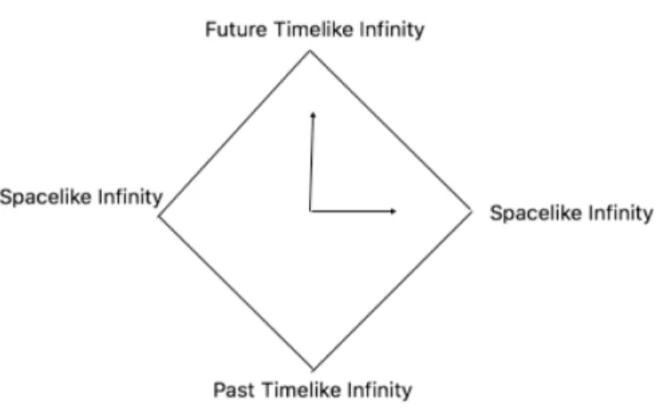
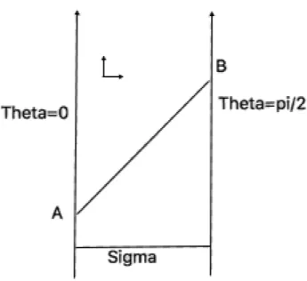
Let us now turn our attention to Anti-deSitter space. Consider the AdSd
metric ds2 = L2cosh2
( )d⌧2+ L2d 2+ L2sinh2
( )d⌦2
d 2, where we have
extended already ⌧ 2 R. Consider the change of coordinates tan(✓) = sinh( ), where ✓ 2 [0,⇡
2], because 2 [0, +1]. The line element is now ds2 = 1
cos2(✓)( d⌧2+ d✓2+ sin2(✓)d⌦2d 2). This is not quite a Penrose
compactifi-cation, since we were unable to bring infinities in ⌧ to finite values (see figure (3)).
Finally, we introduce a new set of coordinates of Anti-deSitter space, called Poincar´e coordinates. As we have seen already, we can view AdSd as the
following surface in R2,d 1, (z1)2+ ( z2+ z3)(z2+ z3) + d+1 X i=4 zi2= L2. (41)
Figure 3: Diagram of AdS space. The vertical coordinate represents ⌧ and the horizontal coordinate ✓. Notice that ✓ 2 [0,⇡
2], while ⌧ 2 R. ⌃ is a spacelike
surface and the line that goes from point A to point B represents the path of a light ray. If we place observers at every point of ⌃, they will be ignorant of the light ray just described, because it does not cross ⌃. Hence, ⌃ is not a Cauchy surface. AdS has no Cauchy surfaces, since, if you draw a spacelike surface, you can always find light rays that travel from lightlike infinity to lightlike infinity without ever crossing that spacelike surface, as this drawing illustrates. Consider the coordinates,
z1= t exp( y L), (42) z2= L cosh( y L) + exp(Ly) 2r (x 2 t2), z3= L sinh(y L) exp(Ly) 2r (x 2 t2), z3+i= xiexp ( y L), with i = 1, ..., d 2and x2 =Pd 2
i=1 x2i. By substituting (42) into the lhs of (41),
we see that indeed we get L2. Yet, notice that we are only parameterizing half
of AdSd, because z2+ z3 = L exp (Ly) > 0. The induced metric is obtained by
putting (42) into the metric of R(2,d 1). We get ds2= exp (2y
Finally, defining the z coordinate such that exp (y L) = L z, we obtain ds2=L 2 z2( dt 2+ dz2+ dx2), (43)
where z goes from 0 to +1.
4.2 Anti-deSitter Black Holes
Anti-deSitter black holes are black hole solutions to the vacuum Einstein equa-tions with a negative cosmological constant. Since our thesis problem is in 4 dimensions, we will restrict our discussion to that case. We start by rewriting the AdS4 metric. Consider the metric as written in (29). Let us extend the
domain of ✓2 to R and do the transformation t = L✓2 and r = L sinh( ). We
obtain ds2= (1 + r 2 L2)dt 2+ dr2 1 +Lr22 + r2d⌦22. (44)
(44) looks similar to the Schwarzschild metric. It turns out that, if we add a ”Schwarzschild term” to this metric, then we obtain the metric
ds2= (1 2M r + r2 L2)dt 2+ dr2 1 2M r + r2 L2 + r2d⌦22, (45)
which is still a solution to the vacuum Einstein equations with a negative cos-mological constant. Notice that this metric contains a black hole, whose horizon is at r⇤, where r⇤ is such that 1 2M
r⇤ +
(r⇤)2
L2 = 0. We observe that, defining
g(r) ⌘ 1 2M
r +
r2
L2, then g0(r) > 0always. Since limr!0g(r) = 1 and
limr!+1g(r) = +1, then g(r) has a root and it is unique. A spacetime with
the metric (45) is called AdS-Schwarzschild.
It is well known that stationary black holes exhibit thermodynamical be-haviour, through the so called laws of black hole mechanics. In particular, a black hole’s temperature T is equal to k
4⇡, where k is the surface gravity. We
now show how to calculate the temperature of black holes with metrics of the type
ds2= f (r)dt2+ 1
f (r)dr
2+ r2d⌦2
2, (46)
where the function f(r) is zero at the horizon. Our method is quick, yet heuris-tic6. An important result in quantum field theory at finite temperature is that
6There’s a more rigorous argument that gives the same result, which involves using the
the partition function of a system at temperature T can be written as the path integral of a quantum field theory, where in the path integral we consider time to be an imaginary and periodic quantity with period 1
T (see [6]). Guided by
that principle, we consider the euclidean version of (46), i.e. we picture time as an imaginary quantity t = i⌧, where ⌧ is a real variable. Near the horizon r⇤,
f (r)⇠ f0(r⇤)(r r⇤), so we define a coordinate ⇢ such that d⇢2= dr2
f0(r⇤)(r r⇤).
More explicitly, we define ⇢ ⌘p(r r⇤)p 2
f0(r⇤). The metric is then
ds2=⇢2f0(r⇤)2
4 d⌧
2+ d⇢2+ r(⇢)2d⌦2
2. (47)
As we mentioned before, ⌧ should be periodic. When ⇢ ! 0, the⇢2f0(r⇤)2
4 d⌧2+
d⇢2portion of the metric should reduce to R2. Thus, ⌧ must have period 4⇡ f0(r⇤),
so the temperature of the black hole isf0(r⇤) 4⇡ .
Let us now see some examples of this formula. For a Schwarzschild black hole, f(r) = 1 2M
r , so T = 1
8⇡M. For a Schwarzschild AdS black hole, after
some algebraic manipulations, we get T = L2+3(r⇤)2 4⇡L2r⇤ .
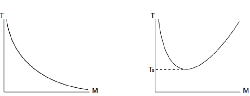
It is instructive to compare the specific heat of Schwarzschild and AdS-Schwarzschild black holes. For AdS-Schwarzschild, @T
@M = 1
8⇡M2. This is negative,
which means that Schwarzschild black holes are unstable thermodynamic ob-jects. To see that, consider putting a Schwarzschild black hole at temperature T in contact with a heat bath at temperature T0. If T0 > T, the heat bath
pro-vides energy to the black hole. Since @T
@M < 0, this causes the temperature of
the black hole to go down, so the system goes away from thermodynamic equi-librium. Analogously, if T0< T, the black hole loses energy, yet its temperature
increases, so once again one deviates from thermodynamic equilibrium. AdS-Schwarzschild black holes don’t suffer from this disease. For them,
@T @M = 3(r⇤)2 L2 4⇡L2(r⇤)2 1 M +(r⇤ )3 L2 , so @T @M is positive if r⇤ > L p
3, which happens for
M > 2 3p3L.
4.3 Some comparisons between gravity in AdS and CFT’s
7We start by comparing the degrees of freedom of a quantum field theory in d
dimensional Minkowski space to a gravity theory in Anti-deSitter space in d + 1 dimensions, using the holographic principle.
Figure 4: At the left, the graph refers to AdS4 and at the right to AdS4
-Schwarzschild. The specific heat of AdS4-Schwarzschild is positive after
M > 2 3p3L.
To simulate a quantum field theory, suppose we arrange a d 1 dimensional cubic lattice, with linear size R and separation between lattice points ✏. The number of degrees of freedom of the quantum field theory are then R(d 1)
✏(d 1)Ns,
where Nsare the number of degrees of freedom per lattice site.
The holographic principle states that the degrees of freedom of a system are contained in its boundary. Specifically, for AdSd+1, it says that the number
of degrees of freedom are equal to A
4GN, where A is the area of the conformal
boundary and GN is Newton’s constant, which has dimensions of [Length]d 1
in units where c = 1 and ~ = 1. A is equal toRz=0;t=t0d
d 1xpg. Now, in
this case, pg = Ld 1
zd 1, which is infinite at z = 0. So, we make the integration
at z = ✏. Also, we say thatRdd 1x = Rd 1. So, the number of degrees of
freedom is Ld 1 4GN(
R ✏)
d 1. This number scales the same way with R and ✏ as it
did for the quantum field theory.
We now prove that the d dimensional conformal group acting on Minkowski space is isomorphic to the group of symmetry of AdSd+1. This provides another
link between conformal field theories in d dimensional Minkowski space and gravity in AdSd+1.
First, we start by defining what is the conformal group. The conformal group is the Lorentz group plus translations, dilatations and special conformal trans-formations. A special conformal transformation generated by a certain vector bµ is the transformation xµ
! x0µ = xµ x2bµ
inversion, after a translation, after an inversion, because xµ x2bµ 1 2b· x + b2x2 = xµ x2 bµ (xµ x2 bµ)2 . (48)
Let us investigate the size of the d dimensional conformal group. It has
d(d 1)
2 Lorentz rotations, plus d translations, d special conformal
transforma-tions and finally 1 dilatation. So, it has(d+1)(d+2)
2 generators, which is the same
number that SO(d, 2) has.
A representation of the conformal group is
Pµ= i@µ, (49)
D = ixµ@µ,
Lµ⌫ = i(xµ@⌫ x⌫@µ),
Kµ= i(2xµx⌫@⌫ x2@µ),
for translations, dilatations, rotations and special conformal transformations, re-spectively. From this, we can deduce its Lie algebra. The nonzero commutators are [D, Pµ] = iPµ, (50) [D, Kµ] = iKµ, [Kµ, P⌫] = 2i(⌘µ⌫D Lµ⌫), [K⇢, Lµ⌫] = i(⌘⇢µK⌫ ⌘⇢⌫Kµ), [P⇢, Lµ⌫] = i(⌘⇢µP⌫ ⌘⇢⌫Pµ), [Lµ⌫, L⇢ ] = i(⌘⌫⇢Lµ + ⌘µ L⌫⇢ ⌘µ⇢L⌫ ⌘⌫ Lµ⇢).
The generators of SO(d, 2) form an antisymmetric tensor JAB, with Lie
al-gebra
[JAB, JCD] = i(⌘ADJBC+ ⌘BCJAD ⌘ACJBD ⌘BDJAC), (51)
where uppercase latin indices go from 1 to d + 2 and the metric ⌘ABis diagonal
with signature { 1, +1, ..., +1, 1}.
such that (51) is obeyed. Define Jµ⌫ = Lµ⌫, (52) Jd+1,µ= Kµ+ Pµ 2 , Jd+2,⌫ = Kµ Pµ 2 , Jd+1,d+2= D,
where the greek indices go from 1 to d and we define JABto be antisymmetric.
It is now a straightforward algebraic computation to show that (51) is satisfied. This proves that indeed the d dimensional conformal group acting on Minkowski space is isomorphic to SO(d, 2).
Suppose we want to calculate the correlation function
< T{O1(x1)...On(xn)} > (53)
of a certain quantum field theory on a fixed background metric. One way of doing that is to add to the lagrangian L(x) the functionsPn
i=1J(x)Oi(x)and
then use < T{O1(x1)...On(xn)} >= 1 Z0 ( i J(x1) )...( i J(xn) )Z[J]J=0, (54)
where Z[J] is the generating functional obtained by the substitution L(x) ! L(x) +Pni=1J(x)Oi(x).
If the background metric is not fixed, like in a quantum theory of gravity, then in the path integral we must also sum over different metrics. The state-ment of AdS/CF T is that, under some assumptions, the generating functional of a conformal field theory in d dimensional Minkowski space is equal to the generating functional of a gravity theory in an asymptotically AdSd+1space.
Furthermore, this duality is often of the strong/weak coupling type and of the quantum/classical type. By that, we mean that it often relates quantum field theories with strong coupling to classical theories of gravity with weak coupling. This means that we can, to good approximation, compute the gener-ating functional on the gravity side by just picking the most probable path and computing exp(iSgrav(gµ⌫, 1, 2, ...)), where gµ⌫, 1, 2, ...are the field
config-urations which solve the equations of motion. Using that, we can then calcu-late functional derivatives and compute correlation functions. The calculation of
Sgrav(gµ⌫, 1, 2, ...)usually involves careful regularization of infinities related
to integrations on the conformal boundary8.
We now derive an important result to our later investigations. In this thesis, we are studying an asymptotically AdS spacetime. So, near the conformal boundary where z = 0, the metric is always
ds2=L2
z2(⌘ µ⌫dx
µdx⌫+ dz2), (55)
where ⌘µ⌫ is the minkowski metric in d dimensions and we are studying AdS
space in d + 1 dimensions. Let us write the KG equation⇤ m2 = 0using
this metric z2 L2(@ 2 z + ⌘µ⌫@µ@⌫ ) (d 1) z L2@z m 2 = 0. (56)
We decompose the scalar field in fourier components
(z, x) = exp (ik· x)fk(z) (57)
and the KG equation becomes
z2fk00(z) (d 1)zfk0(z) (k2z2+ m2L2)fk(z) = 0. (58)
Near z ⇠ 0, k2z2+m2L2
⇠ m2L2. Equation (58) suggests a power law solution.
We try fk(z) = z and we get that the equation is satisfied provided = d
2±
q
(d2)2+ m2L2.
For our present case, plugging d = 3 (spacetime is in dimensions d + 1) and m2= 2
L2 in the last formula9, we obtain = 1and += 2. So, near z ⇠ 0
(z, x) = 1(x)z + 2(x)z2. (59)
The gauge-gravity duality provides a physical meaning to the quantities
1(x)and 2(x). Introducing a scalar field in the gravity theory, corresponds in
the CFT to adding a source termR ddxJ(x)O(x) to the action, where J(x) is
8See [8] for details on this point.
a function we choose (that’s why we call it a source) and O(x) is a scalar op-erator. The gauge gravity duality says that 1(x) = J(x)and 2(x) = hO(x)i,
where hO(x)i is the expectation value for the operator O(x)10.
5 Hovering Black Holes from Charged Defects
Given the great influence it has on our work, we summarize here the main points of [1]. In this paper, solutions of the Einstein-Maxwell equations with a negative cosmological constant were studied, imposing the following boundary conditions. First, it was demanded that spacetime becomes AdS near the con-formal boundary. The second condition is that near z ⇠ 0 the maxwell field Aµ
becomes equal to just µ(r)dt, where µ(r) is a function we choose. In [1], only localized defects were studied, that is, µ(r) ! 0 as r ! 1.
[1] considered profiles where µ(r) goes like a
r , at infinity. Using units where
c =~ = 1, this means that a has dimensions [E]1 . So, if < 1, we will say
that µ(r) is a relevant profile, if = 1, it is a marginal profile and if > 1, it is irrelevant. The reason for this definition is the following. When the profile is irrelevant, the IR horizon is the usual Poincar´e horizon, i.e. it is exactly equal to AdS spacetime there. The IR horizon is the region farther away from the conformal boundary, so in this case this means that the irrelevant profile isn’t strong enough to deform spacetime there. By contrast, for the marginal profile the IR horizon is deformed. Relevant profiles would deform spacetime in the IR horizon so much, that they weren’t studied (their metric there would be very different from AdS)11.
The authors considered the cases where µ(r) is marginal and irrelevant. It turns out that for a large class of profiles in both cases, for sufficiently large a, a Reissner-N¨ordstrom AdS black hole is formed in the bulk. For increasing a, the size of the black hole grows. They could find in this way very large black
10A generalization of this is possible for n-point correlation functions.
11Let us clarify the meaning of this classification with regards to our own work. We study a
massive scalar field, which is a relevant operator in the dimension we’re in. Near the conformal boundary, this scalar field goes like z 1(r), where 1(r)is just some function, which we call a
profile. According to its decay with r ! 1, we say that this profile may be relevant, marginal or irrelevant. This does not change the fact that the scalar field is a relevant operator.
hole solutions, as large as 3L, where L is the AdS radius.
Let a⇤ be the value of a for which a black hole is formed for a certain profile. The main finding of the paper is that, for every profile that exhibits a black hole, the black hole size increases always the same way with a/a⇤. The details of the profile are irrelevant. An explanation for this universality was not provided.
The point of our work was, instead of introducing a boundary maxwell field, studying instead a scalar field.
6 Setup
We study gravity with a scalar field described by the action S = 1 G Z d4xp g(R 2⇤ + 4V ( ) + 2r · r ), (60) where V ( ) = 1 2m 2 2and ⇤ = (d 1)(d 2)
2L2 = L32. Note that is
dimension-less. This gives rise to the following equations of motion Gµ⌫+ 3 L2gµ⌫ ⇣ 2@µ @⌫ + 2V ( ) ⌘ = 0. (61) We choose m2 = 2
L2. Despite being negative, the mass is above the BF
bound, so it induces no instability. This particular value is chosen so that it coincides with the mass of a scalar field conformally coupled to the curvature of AdS4space. Such a field has a mass12
m2= ⇠(d)R = d 2 4(d 1) d(1 d) L2 = d(d 2) 4L2 = 2 L2. (62)
We can now write the ansatz to solve these equations. In order to understand where it comes from, we start by rewriting the metric of the Poincar´e patch of AdS space as
ds2AdS4 =
L2
z2( dt
2+ dz2+ dr2+ r2d 2). (63)
Let us define the polar coordinates z = ⇢ cos ✓, r = ⇢ sin ✓. Then, ds2AdS4= L2 cos2✓( dt2+ d⇢2 ⇢2 + d✓ 2+ sin2✓d 2). (64)
12I do not know a reference for this, but it was proven in the course Topics in Theoretical Physics
Defining ⇢ = 1 ⌘ ds2AdS4 = L2 cos2✓( ⌘ 2dt2+d⌘2 ⌘2 + d✓ 2+ sin2✓d 2). (65)
This way, AdS4is foliated by ⌘ = const slices which are conformal to < ⇥ S2.
Notice that there is now a zero temperature horizon at ⌘ = 0 $ z = 1, r = 1. We call this an IR horizon.
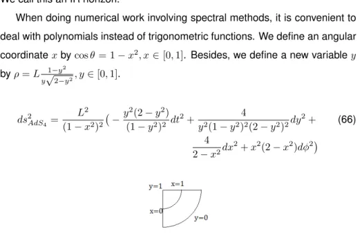
When doing numerical work involving spectral methods, it is convenient to deal with polynomials instead of trigonometric functions. We define an angular coordinate x by cos ✓ = 1 x2, x2 [0, 1]. Besides, we define a new variable y by ⇢ = L 1 y2 yp2 y2, y2 [0, 1]. ds2 AdS4 = L2 (1 x2)2 y2(2 y2) (1 y2)2 dt 2+ 4 y2(1 y2)2(2 y2)2dy 2+ (66) 4 2 x2dx 2+ x2(2 x2)d 2
Figure 5: Poincar´e Patch in the new coordinates. The IR horizon is at y = 0. y = 1is just a point (the corner). The conformal boundary is at x = 1 or y = 1. The axis is at x = 0.
The conformal boundary is at x = 1 or y = 1. Since the metric of our system (with the scalar field) must be asymptotically AdS4, stationary and
axisymmet-ric, we choose the following ansatz ds2= L 2 (1 x2)2 y2(2 y2) (1 y2)2 q1(y, x)dt 2+ 4 y2(1 y2)2(2 y2)2q2(y, x)dy 2+ 4 2 x2q3(y, x)(dx x q5(y, x) y dy) 2+ x2(2 x2)q 4(y, x)d 2 .(67)
The function q5(y, x)allows for a crossed term in the metric. Near the conformal
boundary, the scalar field must go like (z, r) ⇠ z (r), where (r) is a certain profile we choose. We study profiles that decay like B
r . B has dimensions of
[E]1 and so it is said to be relevant if < 1, marginal if = 1 and irrelevant if
= (1 x2)q6(y, x) (68)
This makes our life easier when imposing boundary conditions for the scalar field at the conformal boundary. We remark that the total number of PDE’s that this procedure originates is 6.
7 Boundary Conditions
7.1 Conformal Boundary
The conformal boundary is at x = 1 or y = 1. So, at those places, we put q1=
q2 = q3 = q4 = 1, q5 = 0. The condition for q6 is q6 = L 1 y
2
yp2 y2 (L
1 y2
yp2 y2),
where is the profile that we are considering. At y = 1, q6 = lim✏!0✏ (✏)13.
An important distinction between the marginal and irrelevant case occurs when we consider the boundary condition for q6at x = 1, y = 0. This corresponds to
r! 1. For the marginal case, q6= 0, for the irrelevant case, q6= 0. We will
see that this is important for the IR horizon.
7.2 Regularity Condition at x = 0
We need to impose boundary conditions at x = 0 and y = 0. These come from the fact that we assume all the fields qi to be analytic functions. We
Taylor expand the equations of motion around x = 0 and impose that the zeroth and first order terms be null. We obtain from this that q(0,1)
1 (y, 0), q2(0,1)(y, 0),
q4(y, 0) q3(y, 0), q4(0,1)(y, 0), q (0,1)
5 (y, 0)and q (0,1)
6 (y, 0)are null.
7.3 IR Horizon: irrelevant profile
We consider now the boundary conditions for y = 0. Unlike the x = 0 case, we obtain a set of second order non linear ODE’s in the variables q1(0, x), ..., q6(0, x).
The boundary conditions are the ones we already obtained when we consid-ered the x = 0 and x = 1 case, i.e., at x = 0 all the x derivatives are null and
13If (r) = 0
q3 = q4 and at x = 1, q1= q2= q3= q4= 1, q5= 014. In the irrelevant profile,
q6 = 0at x = 1. Notice that there can be only one solution that solves the set
of ODE’s and respects the boundary conditions.
The simplest guess is to try q1(0, x) = q2(0, x) = q3(0, x) = q4(0, x) = 1,
q5(0, x) = q6(0, x) = 0. It clearly obeys the boundary conditions. It turns out
that it also solves the set of ODE’s, so it is the solution we are looking for. This has a simple interpretation: when the profile is irrelevant it decays quickly and so it does not change the IR horizon, which is still the usual Poincar´e horizon. We bring attention to the fact that the conformal boundary is connected to the IR horizon at x = 1, y = 0 , z = 0, r ! 1, i.e., exactly at the place where the decay of the profile should be most relevant.
7.4 IR Horizon: marginal profile
In the marginal case, q6= 0at x = 1, so the solution for the irrelevant profile
is no longer valid15. We solved the set of ODE’s numerically, according to the
methods explained in section 3.
After knowing q1(0, x), ... q6(0, x), we did a Taylor expansion of scalars like
the curvature, the kretchmann and the norm of the Weyl tensor around y = 0 and calculated the zeroth order term. We graph the maximum along x of all these three quantities as a function of B, as you can see in figures (6), (7) and
(8).
Scalars like the Kretchmann and the curvature increase with B, which
makes sense since the energy momentum tensor goes with 2
B. More
surpris-ingly, W2
⌘ WabcdWabcd, where Wabcd is the Weyl tensor, tends to a constant
for large . As we show in Appendix C, this means that the degrees of freedom contained in the Riemann tensor, which do not depend on the matter field en-ergy momentum tensor, are becoming fixated. We can interpret this as having the metric changing as little as possible with B, given the constraint that the
Einstein equations must be obeyed.
14This can also be seen by taking the non linear ODE’s and Taylor expanding around x = 0 and
x = 1.
15This set of ODE’s has another interesting property. Suppose we take the original Einstein
equations and now assume that the fields qi, i = 1, ..., 6 only depend on x. The equations we
Figure 6: Maximum of the Contraction of the Weyl Tensor in the IR horizon as a function of B
Figure 7: Maximum of the Curvature in the IR horizon as a function of B
As a check on our numerical analysis, we performed a perturbative calcu-lation for small B. See figure 9 for the result and appendix A for the details
Figure 8: Maximum of the Kretchmann Scalar in the IR horizon as a function of
B
Figure 9: Curvature in the IR horizon for B = 0.2. The agreement between
numerical and perturbative methods is total.
8 Bulk Spacetime
16Having discussed the issue of what boundary conditions to impose, we turn
our attention to the numerical solution of the Einstein equations in the bulk. For concreteness, we focus on the irrelevant profile (r) = B
( 2+r2)32, with = 1
in units of L. Like in section 7.4, we can see in figures 10 and 11 how the
maximum value of scalars like the curvature or the Kretchmann scalar increase with B. In figure 12, we sketch the evolution with Bof the norm of the deTurck
vector.
Figure 10: Maximum of the Curvature in the bulk as a function of B. As
expected, it increases with B.
Figure 11: Maximum of the Kretchmann scalar in the bulk as a function of B.
As expected, it increases with B.
A major difficulty in our numerical work is that the norm of the deTurck vector increases with . A way to counter this is to use larger grids for increasing
Figure 12: Maximum of the norm of the deTurck vector in the bulk as a function of B. It is always below the threshold we imposed of 10 10L 2.
B. Because of the computational cost, we were unable to get reliable results
beyond B ⇠ 14.
The maximum of the contraction of the Weyl tensor in the bulk also in-creases with Bfor the range of values we’re considering. See figure 13.
Figure 13: Maximum of the contraction of the Weyl Tensor in the bulk as a function of B.
It is also interesting to investigate the spatial distribution of scalars along the Poincar´e patch. See figure 14, for the case of the curvature.
Figure 14: Absolute value of the curvature. It attains its maximum for x = 0 and y in between 0 and 1.
In analogy to [1], we investigate whether a small AdS-Schwarzschild black hole is formed. It should behave like a particle on a background metric. We thus ask if the metric allows at any Ba static geodesic, that is, a particle that
only moves in the t direction, in our present coordinate system. More precisely, if the particle’s velocity is (p1
gtt, 0, 0, 0), is it ever possible that u
⌫
r⌫uµ = 0?
Symmetry suggests that, if this is to happen, it should happen at the axis at x = 0, because at x 6= 0 the particle needs to choose a certain ' to be in and there’s symmetry in '17. Also, we calculated scalars like the curvature and the
Kretchmann and they all attain their maximum at x = 0. Because of this, we focus on x = 0.
Remembering now that @
@t is a Killing vector and the regularity conditions at
x = 0, @xgtt = 0and gxy = 0, the only nonzero component of u⌫r⌫uµ is the y
component, which gives
17By ' here we mean the angular coordinate and not the scalar field. Hopefully one can tell from
1 2
1 ( gtt)
gyy@y( gtt) (69)
Figure 15: gtthas no maximum, nor minimum, i.e. @ygttis never null at x = 0.
This remains the case for all values of Bthat we have studied.
So, we expect that there is no AdS-Schwarzschild black hole.
We check our numerical work with a perturbative calculation (see appendix
B for details).
Figure 16: Maximum of the Kretchmann Scalar in the bulk spacetime com-puted using numerics and perturbative methods. For small B there’s perfect
9 Discussion and Further Work
Our present work is still very incomplete and there are still a lot of relevant ques-tions to ask. Is there a value of B above which we can not find a solution to
the Einstein equations, just like in [1]? In the limit B ! 1, does the maximum
of the contraction of the Weyl Tensor in the bulk tend to a constant, just like it happens in the IR horizon? We need to extend the calculation we have done in section 8 for larger values of Bin order to answer these questions. Besides,
we should consider other profiles and see if the conclusions from section 8 still hold, namely if an AdS-Schwarzschild black hole is still absent18.
It would be interesting to consider a similar scenario to this one, where in-stead of adding a scalar field to AdS space, we add a scalar field to planar AdS Schwarzschild spacetime. One difference now is that the IR horizon possesses a certain temperature19.
We have seen that the maximum of the contraction of the Weyl Tensor tends to a constant with larger B in the IR horizon and we hypothesize that this is
true in the bulk as well. That would mean that the Riemann tensor is getting as constant as it can, while still satisfying the Einstein equations for different values of B. We could certainly gain a lot of knowledge if we could obtain an
analytical expression for the metric in the limit B! 1.
More broadly speaking, there are further problems we could takle which are related to this study. One of them is generalizing the deTurck gauge for non stationary spacetimes. This would be very helpful, as it would enable us to study gravity in AdS space in a dynamical setting using spectral methods.
Appendix
A - Perturbative Calculation for ODE’s
We calculate the metric for small B. Our method is the following. First, we
use the metric of AdS space and write with it the Klein Gordon equation for
18We have already made some numerical calculations and until now that conclusion still holds,
but a systematic study is needed.
19The study of a maxwell field coupled to a charged complex scalar field in planar AdS
the scalar field. We solve this equation to linear order in B. Armed with this
knowledge, we calculate the energy momentum tensor to order 2
B. Now we
solve the Einstein equations to order 2
B, i.e., we obtain the metric to order 2
B. We have now gone full circle and we can use the metric to order 2B to
obtain the scalar field to order 3
B and then use that to obtain the metric to
order 4
Band so on... The point here is that the energy momentum tensor Tµ⌫
is quadratic in the scalar field ,
Tµ⌫= gµ⌫ @ · @ + 2V ( ) + 2@µ @⌫ . (70)
We will now explain this procedure more carefully. First, we remark that not all the six fields qi, i = 1, ..., 6are non zero and independent at the IR horizon.
In fact, q5(0, x) = 0and q1(0, x) = q2(0, x)20. Redefining q3 ! q2and q4! q3,
let us write21
q1(x) = 1 + a1(x) B+ a2(x) 2B+ ... (71)
q2(x) = 1 + b1(x) B+ b2(x) 2B+ ... (72)
q3(x) = 1 + c1(x) B+ c2(x) 2B+ ... (73)
(x) = d1(x) B+ d2(x) 2B+ .... (74)
Since at x = 1 spacetime must be AdS, ai(1) = bi(1) = ci(1) = 0. Also, at
x = 0we impose the regularity conditions written in section 7.2.
Using this, we can now make similar expansions for the energy momentum tensor, the metric, the box operator and the Riemann tensor, with the result
Tµ⌫= Tµ⌫(2) 2B+ Tµ⌫(3) 3B+ Tµ⌫(4) 4B+ ... (75)
gµ⌫ = g(0)µ⌫ + g(1)µ⌫ B+ g(2)µ⌫ 2B+ gµ⌫3 3B+ ... (76)
⇤ = ⇤(0)+⇤(1)
B+⇤(2) 2B+ ... (77)
Rµ⌫ = R(0)µ⌫ + R(1)µ⌫ B+ Rµ⌫(2) B2 + Rµ⌫(3) 3B+ Rµ⌫(4) 4B+ .... (78)
Let us see how this works explicitly to order 2. At the beginning, we only know
20I know that I can solve the set of ODE’s by imposing these conditions, but I’m unaware of a
physical reason why this must be true.
21In this case, it is not convenient to put = (1 x2)q 6(x)
all the zeroth order terms. The KG equation to linear order is
(⇤(0) m2) (1)(x) = 0, (79) with the boundary conditions that (1)(x)goes like 1 x2 near x = 122 and
the derivative of (1)(x) at x = 0 equals 0. We solve this ODE and obtain (1)(x) = 1 x2.
The Einstein equations, to linear order, are G(1)
µ⌫ + ⇤gµ⌫(1)= 0. (80)
The boundary conditions are that g(1)
µ⌫ must be null at the conformal boundary
and that it should obey the regularity conditions at x = 0. The equations (80) are a homogeneous set of ODE’s, i.e., they contain no source term. Together with the boundary conditions, they imply g(1)
µ⌫ = 0. Hence,⇤(1)= 0.
The KG equation to second order is
(⇤(0) m2) (2)= ⇤(1) (1), (81)
with the boundary conditions that (2) is null at x = 1 and its derivative is zero
at x = 0. Also, the rhs of (81) is null, since⇤(1)= 0. So, (2)= 0.
We can now obtain T(2)
µ⌫. Writing the Einstein equations to second order,
we will obtain a non homogeneous set of ODE’s for g(2)
µ⌫. The equations are
8x(x2 1)2a2(x) 8x(x4 2x2 2)b2(x) + (x2 1) ⇣ ( 5x4+ 11x2+ 2)a02(x) +x (x2 1)((x2 2)a002(x) + 16) + 2x(x2 2)b02(x) 2x(x2 2)c02(x) ⌘ = 0 24xb2(x) + (x2 1) 4a02(x) 2b02(x) + 4c02(x) + 16x3 16x x5c002(x) 3x3c002(x) + 2xc200(x) x4c02(x) + 3x2c02(x) = 0 2x x2 1 2a 2(x) + 2x x4 2x2 2 b2(x) + x2 1 x4 2x2 1 a02(x) + x x x2 2 c02(x) + 2 x6 3x4+ 2 = 0 (82) These equations are not elliptic, as a b00(x)term is missing. Notice we have
not imposed the deTurck gauge, so this is natural. Let’s solve the third equation for b2(x)and plug that into the first two equations.
22This amounts to demanding that near the conformal boundary, the scalar field goes like z 1(r)
b2(x) = 1 2x (x4 2x2 2)(x 2 1) 2x x2 1 a 2(x) + x4 2x2 1 a0 2(x) + x x x2 2 c02(x) + 2 x6 3x4+ 2 ( 1 + x2) 24x3 x2 1 a2(x) + 9x6+ 19x4+ 4x2 2 a02(x) + x x x8 5x6+ 10x4 6x2+ 12 c02(x) + x6 3x4+ 2 a002(x) + x2 2 x2c002(x) = 0 (1 + x2 3x4+ x6) 24x3 x2 1 a2(x) + 9x6+ 19x4+ 4x2 2 a0 2(x) + x x x8 5x6+ 10x4 6x2+ 12 c02(x) + x6 3x4+ 2 a002(x) + x2 2 x2c002(x) = 0. (83) Clearly, the last two equations are equivalent. To make progress, we must choose a gauge. Our philosophy during this section will be to impose a gauge order by order. That way, we can look at the equations and choose. We put c2(x) = ↵a2(x). To order 2, ↵ is a gauge variable, i.e., when we calculate
scalars like the curvature or the kretchmann they will not depend on ↵ to order 2. Yet, if we want to proceed with the calculation to higher order, we will have to fix ↵, so in that sense it is not a gauge variable. Solving the equations (83) and imposing the boundary conditions, we obtain
a2(x) = (x 2 1)3 2↵x4 4↵x2 2, b2(x) = 1 ( ↵x4+ 2↵x2+ 1)2 x 2 1 2 ✓ 1 2( ↵ 2) + 1 ↵2x8 7↵2x6 2 + ✓5↵ 2 2 ◆ ↵x4 ✓ ↵2 9↵ 2 1 ◆ x2), c2(x) = ↵ x 2 1 3 2↵x4 4↵x2 2. (84)
No new methods are involved in going to higher orders, so we will not show the details here. We calculated expressions up to order 4. In order 5, we started to encounter dilogarythms and so we stopped.
As we have seen, for B= 0.2this expansion works well. For larger values,
![Figure 1: Suppose we want to approximate a function f (x), where x 2 [ 1, 1].](https://thumb-eu.123doks.com/thumbv2/123dok_br/18903861.935617/16.918.349.538.735.894/figure-suppose-want-approximate-function-f-x-x.webp)