MATHEMATICAL AND NUMERICAL METHODS FOR INVERSE
PROBLEMS USING FUNDAMENTAL SOLUTIONS TECHNIQUES
Disserta¸c˜ao apresentada para obten¸c˜ao do Grau de Doutor em Matem´atica, especialidade An´alise Num´erica, pela Universidade Nova de Lisboa, Faculdade de Ciˆencias e Tecnologia.
Acknowledgements
I’m grateful to the Faculdade de Ciˆencias e Tecnologia (UNL) and in particular to the department of mathematics for conceding me a three years leave to do this work. In this period, I was also supported by Funda¸c˜ao para a Ciˆencia e Tecnologia (MCES) through the scholarship SFRH/BD/27914/2006.
I thank my advisor, Professor Carlos Alves, for accepting me at his research group in CEMAT. I was a complete stranger to both inverse problems and meshfree methods (and in fact to Prof. Alves) and he had the patience to guide my first steps in these worlds.
I started my first steps in the world of numerical analysis with Professor Elvira Coim-bra, while a licenciatura student. My interest for numerical analysis grew when I became teaching assistant at a numerical analysis course gave by her. It has been a pleasure to be able to work with both.
I thank my ”old” friends from the department of mathematics (FCT–UNL), my not so old friend from the Mestrado course in applied mathematics at IST and my (not so new) Ph.D. colleages from IST. Either discussing scientific work or simply talking nonsense at the most strange places it has always been fun.
I can’t seem to find the exact word to thank the support of my family (both old and new). It is even harder to fully express my gratitude to my wife M´onica and our son Vasco for the patience (and impatience) as I neared the completion of this work.
Resumo
Neste trabalho s˜ao estudados m´etodos matem´aticos e num´ericos para problemas inversos relacionados com a identifica¸c˜ao e reconstru¸c˜ao de forma, recupera¸c˜ao de coeficientes de Robin e fontes a partir de medi¸c˜oes na fronteira. Numa primeira fase, a identifica¸c˜ao de formas e coeficientes ´e estudada num contexto de problemas de valores na fronteira para a equa¸c˜ao de Laplace, num dom´ınio limitado Ωc. A fronteira de Ωc ´e dada pela reuni˜ao de duas curvas fechadas e regulares Γ (exterior) eγ (interior). Emγ, considera-se uma condi¸c˜ao de fronteira homog´enea do tipo Dirichlet ou Neumann. Demonstra-se que a partir de dados de Cauchy num conjunto relativamente aberto Σ⊂Γ ´e poss´ıvel identificar γ e a condi¸c˜ao de fronteira a´ı definida. Apresenta-se um crit´erio que permite distinguir a condi¸c˜ao de fronteira emγ a partir de um par de dados de Cauchy em Γ. Desenvolvem-se dois m´etodos num´ericos para a resolu¸c˜ao do problema inverso geom´etrico (reconstru¸c˜ao deγ), considerando em γ ⊂R2 uma condi¸c˜ao de Dirichlet homog´enea. O primeiro, ´e um
m´etodo que consiste na separa¸c˜ao da parte mal posta (por interm´edio da resolu¸c˜ao de um problema de Cauchy) da parte n˜ao linear (m´etodo de decomposi¸c˜ao). O segundo, ´e um m´etodo iterativo do tipo quasi–Newton que requer a resolu¸c˜ao de v´arios problemas directos por cada iterada. Prop˜oe-se a aplica¸c˜ao do m´etodo das solu¸c˜oes fundamentais para a resolu¸c˜ao num´erica problemas anteriores (Cauchy e directos) e s˜ao apresentadas v´arias simula¸c˜oes num´ericas para testar estes dois m´etodos.
Seguidamente, considerando uma condi¸c˜ao homog´enea mista em γ estuda-se o prob-lema inverso de identificar o coeficiente de Robin na fronteira γ (que agora se sup˜oe ser conhecida) a partir de um par de dados de Cauchy em Σ⊂Γ. Estuda-se uma adapta¸c˜ao dos m´etodos de decomposi¸c˜ao e quasi–Newton anteriormente propostos e apresentam-se v´arias simula¸c˜oes num´ericas para testar e comparar os resultados obtidos atrav´es destes m´etodos.
Os m´etodos matem´aticos e num´ericos apresentados para o problema de Laplace s˜ao estudados e implementados para os correspondentes problemas geom´etrico e de Robin em elasticidade linear (sistema de Lam´e).
Abstract
In this work we study mathematical and numerical methods for inverse problems related with the identification and reconstruction of shapes, boundary coefficients and sources from boundary measurements. The geometric and coefficient problem is studied in the context of a boundary value problem for the Laplace equation in a non simply connected bounded domain Ωc. The boundary of Ωc is the union of two regular closed curves Γ (exterior) and γ (interior). Assuming a homogeneous Dirichlet or Neumann boundary condition on γ, we show that from a single pair of Cauchy data on an accessible part of the boundary Σ ⊂ Γ we can identify both the boundary condition and the boundary γ. A criterion is presented to distinguish such situations. We study two numerical methods to retrieveγ in the two dimensional case, when considering a homogeneous Dirichlet con-dition on γ. The first is a decomposition method requiring at a first step the resolution of a Cauchy problem. The second is a Quasi–Newton method that requires the resolution of several direct problems. For both situations, we propose the method of fundamental solutions as numerical approximation for the Cauchy and direct problems. Several numer-ical examples are presented and the accuracy and robustness of the methods is discussed. Considering a homogeneous Robin condition on γ, we address the inverse problem that consists in the identification of the Robin coefficient onγ (the boundary is now assumed to be known) from a single pair of Cauchy data on Γ. An adaptation of the decomposition and Quasi–Newton methods is studied and implemented. Several numerical simulations are presented to illustrate and compare the performance of both methods.
The previously developed mathematical and numerical methods are studied in the corresponding geometric and coefficient problems for the Lam´e system. The last chapter concerns the identification of acoustic sources from boundary measurements. We show that, from many boundary measurements, identification may not be possible and we propose the use of data generated from many wave numbers. To solve this linear problem, we describe and implement a numerical method based on the reciprocity gap functional. The method is illustrated with several numerical simulations.
Notation and abbreviations
| | Euclidean norm of a vector in Rd
h, iH inner product in a Hilbert space H
|| ||H the norm of a vector in a Hilbert space H
h, iH×H′ duality pairing between H and the dualH
′ u·v the product defined by u·v:=Pdi=1uivi
∆ Laplacian
dx the infinitesimal volume element dx1. . . dxd
dς the infinitesimal surface element
BVP boundary value problem(s)
KKM Kirsch Kress method
MFS method of fundamental solutions PDE partial differential equation(s)
n, nx the unit normal vector pointing outward on the boundary of a regular bounded domain (atx)
Ω an open set in Rd: Ω is connected and bounded with regular boundary
Γ =∂Ω
Ω the closure of Ω
ΩC the complement of Ω in Rd
C0(Ω) space of continuous functionsf : Ω−→R
Ck(Ω) space of k– times continuously differentiable functionsf : Ω−→R Ck(Ω,Rd) k– times continuously differentiable functionsf : Ω−→Rd
Hr(Ω) the Sobolev space of orderr on Ω Hr(Ω) the Sobolev space (Hr(Ω))d
L2(Ω) the Hilbert space of square integrable functions on Ω
L2(Ω) the Hilbert space (L2(Ω))d
Contents
1 Introduction 1
2 Preliminary results 5
2.1 Poisson equation . . . 5
2.1.1 Fundamental solutions . . . 8
2.1.2 Integral representation . . . 8
2.2 Helmholtz equation . . . 11
2.2.1 Fundamental solutions . . . 13
2.2.2 Integral representation . . . 13
2.3 Elasticity system . . . 14
2.3.1 Fundamental tensors . . . 16
2.3.2 Elastostatic potentials . . . 16
2.4 Inverse problems . . . 18
2.4.1 Ill–posedness and regularization . . . 18
2.4.2 Ill conditioning in inverse and direct problems . . . 22
3 Obstacle identification from a single measurement for a Laplace problem 25 3.1 Geometric problem . . . 26
3.1.1 Inverse problem . . . 28
3.1.2 Local Lipschitz stability . . . 32
3.2 Robin problem . . . 39
3.2.1 Inverse problem . . . 41
3.2.2 Local Lipschitz stability . . . 44
3.3 Conclusions . . . 46
4 The MFS for direct and inverse problems - Laplace equation 47 4.1 The MFS for direct problems . . . 48
4.1.2 Numerical simulations . . . 56
4.2 A MFS based decomposition method for the inverse geometric problem . . 65
4.2.1 The MFS for the inverse (Cauchy) problem . . . 65
4.2.2 Numerical implementation . . . 68
4.2.3 Numerical simulations . . . 72
4.3 Iterative reconstruction of the inclusion by a Quasi–Newton method . . . . 80
4.3.1 Numerical simulations . . . 85
4.4 The MFS applied to the inverse Robin problem . . . 97
4.4.1 Decomposition method . . . 97
4.4.2 Numerical simulations . . . 99
4.4.3 Iterative reconstruction of the coefficient by a Quasi–Newton method104 4.4.4 Numerical simulations . . . 107
4.5 Conclusions . . . 110
5 Identification and MFS reconstruction of obstacles - linear elasticity 113 5.1 Geometric problem . . . 114
5.1.1 Inverse problem . . . 114
5.2 Robin problem . . . 115
5.2.1 Inverse Robin problem . . . 117
5.3 The MFS approximation for direct problems in linear elasticity . . . 118
5.3.1 Numerical implementation . . . 119
5.3.2 Numerical simulations . . . 120
5.4 Application of the decomposition method to the elastic geometric inverse problem . . . 126
5.4.1 Numerical simulations . . . 127
5.5 Application of the optimization method to the elastic geometric problem . 133 5.5.1 Numerical simulations . . . 136
5.6 Decomposition method for the inverse Robin problem . . . 145
5.6.1 Numerical simulations . . . 146
5.7 Conclusions . . . 148
6 Identification and source reconstruction from boundary data 149 6.1 Direct and inverse problem . . . 150
6.2 Restricted identifiability with a single wave number . . . 150
6.2.1 Identification in linear/affine classes . . . 152
6.3 Identification of sources using multiple frequencies. . . 157
6.5 Numerical implementation for the direct problem . . . 159
6.5.1 Numerical examples . . . 160
6.6 Reconstruction of a source using the reciprocity gap functional . . . 163
6.6.1 Numerical examples . . . 165
6.7 Conclusions . . . 172
Final remarks and future work 173
Appendix: Levenberg–Marquardt method for non linear least squares
prob-lems 175
List of Figures
3.1 Example of a domain of propagation Ωc ⊂R2. . . . 26
3.2 Examples for the chosen σ, when Ω1 c∩Ω2c is connected (left) and not con-nected (right). . . 31
3.3 A deformation of Ωc by the diffeomorphism Ψε. . . 33
3.4 Plot of the functions from Example 3.15. . . 42
4.1 A doubly connected domain Ωc and an artificial boundary Γb∪bγ. . . 49
4.2 Geometry of the domains. The black dots represent the source points (direct problem). . . 58
4.3 Absolute error on the boundary (direct problem). . . 59
4.4 Absolute error on the boundary (direct problem). . . 59
4.5 Absolute error on the boundary (direct problem). . . 60
4.6 Absolute error on the boundary (direct problem). . . 60
4.7 Geometry of the domain for the Robin problem. The blue line represents the boundary of∂Ωcand black dots the location of the point sources (direct problem). . . 62
4.8 Considered Robin coefficients. . . 63
4.9 Error on the boundary - Example 1 (direct problem). . . 64
4.10 Error on the boundary - Example 2 (direct problem). . . 64
4.11 Error on the boundary - Example 3 (direct problem). . . 64
4.12 Limit situation where the operator matrix arising from the direct MFS (on the left), M(Γ, γ), formally tends toM(Γ,Γ), the matrix arising from the KKM, used as a Cauchy solver in a different region of interest (on the right). 66 4.13 Example of noise free data. . . 71
4.14 Example of the above data with noise. . . 72
4.15 Left– segment defined by two points on Γ and bγ2 (black dots). Right– solution of the inverse problem along the line of the left plot. The red dot is the computed approximation. . . 74
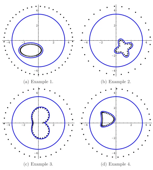
4.16 Reconstruction of the shape considering noise free data. . . 75
4.17 Reconstruction of the shape considering noise free data. . . 75
4.18 L–curve for the first example. The red dot corresponds to the selected value for regularization parameter. . . 76
4.19 Dirichlet data fitting with the MFS. . . 76
4.20 Neumann data fitting with the MFS. . . 76
4.21 Reconstruction of the ellipsis from noisy data. . . 77
4.22 Reconstruction of the ellipsis from noisy data. . . 77
4.23 Comparison between the reconstruction of γ2 using the proposed internal curve (left) and bγ2 =∂B(c2,0.5) (right). Noise level: 5%. . . 78
4.24 Reconstruction of γ2 from noisy data (Noise level: 10 %). . . 79
4.25 Reconstruction of γ3 from noisy data. . . 79
4.26 Reconstruction of γ4 from noisy data. . . 80
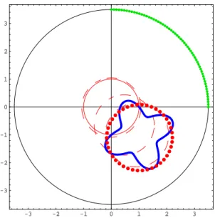
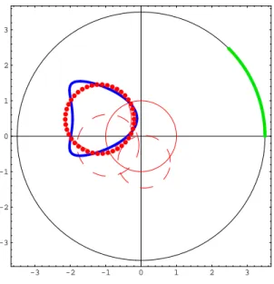
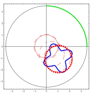
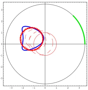
4.27 Reconstruction of γ1 (left) and γ2 (right) inC4 for data without noise. . . . 86
4.28 Reconstruction of γ3 in C0 (left) and C4 (right) for data without noise. . . . 87
4.29 Reconstruction of γ4 in C4 for data without noise. . . 87
4.30 Reconstruction of γ1 in C4. . . 88
4.31 Reconstruction of γ1 in C4. . . 89
4.32 Reconstruction of γ2 in C4. . . 90
4.33 Reconstruction of γ3 in C0 (left) and C4 (right). Noise level: 5 %. . . 91
4.34 Reconstruction of γ3 in C0 (left) and C4 (right). Noise level: 10 %. . . 91
4.35 Reconstruction of γ4 in C4. . . 92
4.36 Reconstruction of γ2 in C0 from incomplete noise free data. . . 93
4.37 Reconstruction of γ2 in C0 (left) and C4 (right) from incomplete noise free data. . . 93
4.38 Reconstruction of γ4 in C0 from incomplete noise free data. . . 94
4.39 Reconstruction of γ4 in C0 (left) and C4 (right) from incomplete noise free data. . . 94
4.40 Reconstruction of γ2 in C0 from incomplete noisy data. Noise level: 5 %. . 95
4.41 Reconstruction of γ2 inC0 (left) andC4 (right) from incomplete noisy data. Noise level: 5 %. . . 96
4.42 Reconstruction of γ4 in C0 from incomplete noisy data. Noise level: 5 %. . 96
4.43 Reconstruction of γ4 inC0 (left) andC4 (right) from incomplete noisy data. Noise level: 5 %. . . 97
4.44 Reconstruction of the Robin coefficient from noise free boundary data. . . 99
4.45 Reconstruction of Z3 from noise free boundary data. . . 99
4.47 Reconstruction of Z2 from noisy data. . . 101
4.48 Reconstruction of Z3 from noisy data. . . 102
4.49 Error of the Cauchy data fitting from partial data. . . 102
4.50 Reconstruction of Z2 from partial noise free boundary data. . . 103
4.51 Reconstruction of Z3 from partial noise free boundary data. . . 103
4.52 Reconstruction of Z2 from partial noisy boundary data. Noise: 5% . . . 103
4.53 Reconstruction of Z3 from partial noisy boundary data. Noise: 5% . . . 104
4.54 Iterative reconstruction of the Robin coefficient inC4 from noise free bound-ary data. . . 108
4.55 Iterative reconstruction of Z3 in C4 from noise free boundary data. . . 108
4.56 Iterative reconstruction of Z1 in C4 from noisy boundary data. . . 109
4.57 Iterative reconstruction of Z2 in C4 from noisy boundary data. . . 109
4.58 Iterative reconstruction of Z3 in C4 from noisy boundary data. . . 110
4.59 Iterative reconstruction of Z2 in C4 from data measured on the arc [0, π/2]. 110 5.1 Geometry of the domains and distribution of point sources (direct problem).121 5.2 Absolute error on Γ - First example (direct problem). . . 122
5.3 Absolute error onγ - First example (direct problem). . . 122
5.4 Absolute error on Γ - Second example (direct problem). . . 122
5.5 Absolute error onγ - Second example (direct problem). . . 123
5.6 Absolute error on Γ - Third example (direct problem). . . 123
5.7 Absolute error onγ - Third example (direct problem). . . 123
5.8 Error on Γ - Example 1 (direct problem). . . 125
5.9 Error on γ - Example 1 (direct problem). . . 125
5.10 Error on Γ - Example 2 (direct problem). . . 125
5.11 Error on γ - Example 2 (direct problem). . . 126
5.12 Reconstruction of the elastic inclusion for the first example using the de-composition method (noise free data). . . 128
5.13 Reconstruction of the shape considering noise free data. . . 129
5.14 Reconstruction of γ1 from noisy data. . . 129
5.15 Reconstruction of γ2 from noisy data. . . 130
5.16 Reconstruction of γ3 from noisy data. . . 131
5.17 Reconstruction of γ2 from incomplete noise free data. . . 132
5.18 Reconstruction of γ3 from incomplete noise free data. . . 132
5.19 Reconstruction of γ2 from incomplete noisy data (noise level: 5%). . . 133
5.20 Reconstruction of γ1 inC0 (left) andC4 (right) from data without noise. . . 137
5.22 Reconstruction of γ3 in C0 (left) and C4 (right) from data without noise. . . 138
5.23 Reconstruction of γ1 in C0 (left) and C4 (right) from data with 5% of noise. 139
5.24 Reconstruction of γ1 in C0 (left) and C4 (right) from data with 10% of noise.139
5.25 Reconstruction of γ2 in C0 (left) and C4 (right) from data with 5% of noise. 140
5.26 Reconstruction of γ2 in C0 (left) and C4 (right) from data with 10% of noise.140
5.27 Reconstruction of γ3 in C0 (left) and C4 (right) from data with 5% of noise. 141
5.28 Reconstruction of γ3 in C0 (left) and C4 (right) from data with 10% of noise.141
5.29 Reconstruction of γ2 in C0 (left) and C4 (right) from incomplete noise free
data. . . 142 5.30 Reconstruction of γ2 in C0 (left) and C4 (right) from incomplete noise free
data. . . 143 5.31 Reconstruction of γ3 in C0 (left) and C4 (right) from incomplete noise free
data. . . 143 5.32 Reconstruction of γ3 in C0 (left) and C4 (right) from incomplete noise free
data. . . 144 5.33 Reconstruction of γ2 in C0 (left) and C4 (right) from incomplete data with
5% of noise. . . 144 5.34 Reconstruction of γ2 in C0 (left) and C4 (right) from incomplete data with
5% of noise. . . 145 5.35 Reconstruction of the Robin coefficient from noise free boundary data. . . 146 5.36 Reconstruction of Z1 with the explicit formulation (data with 5 % of noise).147
5.37 Reconstruction in C4 from data with 5 % of noise. . . 147
5.38 Reconstruction of Z2 from incomplete noise free data. . . 148
6.1 Plot of the sources in Ω. . . 161 6.2 Distribution of collocation and source points. The black dots represent
source points, the red dots represent collocation points and the full blue line is the boundary of the domain. . . 161 6.3 Absolute error for the approximation of f1 (left) and the approximation of
the boundary condition (right). . . 162 6.4 Absolute error for the approximation of f2 (left) and the approximation of
the boundary condition (right). . . 163 6.5 Absolute error of the boundary condition approximation for the third
ex-ample. . . 163 6.6 Reconstruction of f1 considering noise free data obtained from a single
6.7 Reconstruction off1 considering noise free data obtained from several
mea-surements. . . 166 6.8 Reconstruction off1 considering data with several levels of noise, obtained
from three measurements. . . 167 6.9 Reconstruction off2 considering noise free data obtained from several
mea-surements. . . 169 6.10 Reconstruction off2 considering data with 5% of noise obtained from three
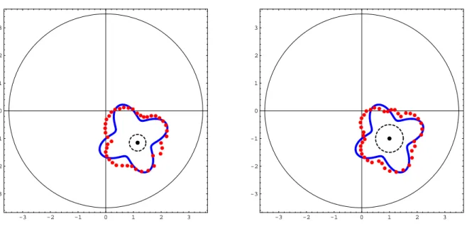
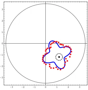
measurements. . . 170 6.11 Contour plot regarding the reconstructions of f2 considering three
bound-ary measurements. . . 170 6.12 Reconstruction of four points sources considering noise free data obtained
from several boundary measurements. . . 171 6.13 Reconstruction of four points sources considering data with 5% of noise
obtained from four boundary measurements. . . 171 6.14 Contour plot regarding the reconstruction of four points sources (red dots)
List of Tables
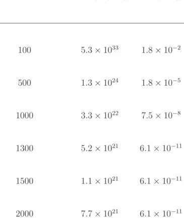
4.1 Evolution of the condition number and the error on the boundary with the number of collocation points, for example 2. . . 61 4.2 Distinguishing an inclusion from a cavity by the value of RΓgndς. . . 73
1
Introduction
The study of inverse problems in partial differential equations is an area of intensive research in our days. From the mathematical point of view, these problems are quite challenging due to their ill–posed nature. In the early work of Hadamard (cf. [46]), ill– posed problems were believed to be incorrectly posed, ”artificial” and that they would not describe physical systems. Many properly formulated inverse problems arise from physical systems. The successful non intrusive medical imaging, discovery of oil reservoirs from seismic measurements (to name a few) are a proof that, despite several mathematical and computational challenges, we can in fact obtain some meaningful information from boundary or exterior measurements. Moreover, one should have in mind that, in practise, a mathematical model (in our case a PDE) is used to describe the physical problem and tested with real measured data. Assuming that the model describes the physical system accurately, two natural questions arise:
1) How many measurements must we consider in order to identify the object?
2) If two measurements that are in some sense close to each other were generated by two objects can we still expect that the objects are ”close” to each other ?
The first is an identifiability question and the second a stability question and are two of the main theoretical questions for the inverse problem.
In inverse problems, the existence issue is inherent to its formulation, in two aspects: i) we assume that the measured data is given (ie. a solution exists);
ii) the measurements are not exact, are affected by noise (ie. a solution that produces such results does not exist).
Robust numerical methods are also very important. If on one hand we need fast and accurate numerical solvers on the other the method has to be sufficiently robust to deal with the ill posedness. If for the robustness issue regularization methods are usually applied (with good results) the search for a fast accurate (and easy to implement) numerical solver for the underlying PDE is very important.
The method of fundamental solutions (MFS) is a meshfree numerical method usually applied to solve certain boundary value problems. The approximation is given by a linear combination of several shifted fundamental solutions that automatically solve the PDE (here we shall consider Laplace and Helmholtz equations and the Lam´e system) and therefore one only has to fit the boundary condition(s). The method has the three aforementioned properties for the addressed problems: is easy to implement, is a fast solver and for sufficiently regular boundaries and boundary data it produces excellent results.
In this work we study several inverse problems related to the identification of sources, boundary coefficients and shape from measurements on an accessible part of the boundary. The study is complemented with several numerical methods relying on the MFS and numerical examples are provided to illustrate the feasibility of the methods. The work is organized as follows:
We start with some useful results or concepts that will be used through the work (Chapter 2).
In Chapter 3 we study two inverse problems that can serve as a model for detection of corrosion from boundary measurements. The domain is a two connected set with interior boundary γ and exterior boundary Γ. Inside, Laplace equation holds and on Γ we have a Dirichlet condition.
not identically constant, a single pair of (compatible) Cauchy data is sufficient to identify γ. We extend this result and show that under the same assumptions we can identify both boundary shape γ and boundary condition on γ. We present a criterion to distinguish such boundary conditions from the Cauchy data on Γ. The well known expression for the domain derivative for the Dirichlet problem is derived and as a consequence, the local Lipschitz stability result.
The second part of this chapter is devoted to the identification of a Robin boundary coefficient Z on γ from Cauchy data on Γ. This Robin problem is similar to other Robin problem addressed by several authors in the literature (eg. [50], [33]) and the identifiability, derivative expression and Local Lipschitz stability results were established using the same type of arguments.
Chapter 4 is devoted to the MFS and its applications to direct and inverse problems and is complemented with several numerical simulations. First a theoretical study of the MFS for the Laplace equation in two connected domains and an application to direct problems in such domains. Several numerical examples are provided with the twofold objective of showing the accuracy of the method for several boundary value problems and to obtain artificially generated boundary measurements for the inverse problem.
The second part is devoted to MFS based methods for the inverse geometric and Robin problems. The methods can be divided in two categories: decomposition based methods and Newton–type of methods.
The first decomposes the ill posedness and non linearity of the inverse problem in two steps. The ill posedness is addressed by solving the linear Cauchy problem. Although several authors have used the MFS as Cauchy problem solver (eg. [52], [67]), to our knowledge, no direct theoretical proofs regarding this numerical approximation have been provided. We provide such results in section 4.2.1 and establish a connection with the MFS approximation for the direct problem. The numerical method for the inverse geometric problem consists in computing an approximate solution for the Cauchy problem and a line search method, based on maximum principle results, to reconstruct the shape of γ. Several numerical examples are presented in order to illustrate the feasibility of the method.
A Levenberg–Marquardt optimization method based on the MFS approximation for direct problems is proposed for the inverse geometric problem. We implemented the proposed method and compared the results with those of the decomposition method. Numerical tests with partial data were also considered.
The decomposition approach provided a simple reconstruction method for the Robin problem. The Levenberg–Marquardt method was adapted to the Robin problem and a numerical comparison of both methods is presented (for complete and incomplete Cauchy data).
The mathematical study of the geometric and Robin (inverse) problems for the elasto-static problem is addressed in Chapter 5 where the MFS based methods described in the previous chapter are extended to the Lam´e system. This chapter is based on the papers [13] and [14].
2
Preliminary results
This introductory chapter surveys useful results concerning the partial differential equa-tions that will be used in the following chapters and some discussion about inverse prob-lems and ill posedness. Since we will be dealing mainly with interior probprob-lems, we start with the definition of domain.
Definition 2.1 We define (interior) domain as an open, bounded and connected set Ω⊂Rd with regular boundary Γ :=∂Ω (at least C1).
We will address the casesd= 2,3. We recall that on a regular boundary Γ, the normal vector n is defined at each point. In this work, we will always assume that the normal vector points outward with respect to the domain Ω.
2.1
Poisson equation
Poisson equation or potential equation
∆u=f in Ω (2.1)
is the classical example for second order elliptic partial differential equations and it is a mathematical model to some important physical phenomena. For instance:
• Gravitation problems: u is the gravitation field generated by the mass distribution f.
• Conductivity problems: For a body with constant electric or thermal conductivity K,uis the electric or thermal potential and, for a given source f, we have Poisson’s equation
∆u=f /K.
In absence of sources, that is f ≡0, equation (2.1) is called Laplace equation. These equations may have several solutions and some extra condition(s) must be considered.
The usual boundary conditions for the Poisson equation are: • Dirichlet:
u=g on Γ.
This means that the temperature (in thermal conductivity problems) or the voltage (electrostatic problems) is imposed.
• Neumann:
∂nu=g1 on Γ,
wheren is the outward unit normal to the boundary and ∂nuis the normal
deriva-tive on Γ. With this condition we impose heat flux (thermal problems) or current (electrostatic).
• Robin:
∂nu+Zu=g1 on Γ,
which is a more general boundary condition. We note that, for the Robin coefficient Z = 0 we obtain the Neumann condition and for Z =∞the Dirichlet condition. The following are the well known Hopf’s lemma and strong maximum principle for Laplace equation. For a proof, see [37].
Lemma 2.2 (Hopf ’s lemma) Let u∈ C2(Ω)∩C0(Ω) be a function satisfying Laplace’s
equation in a domain Ω with C2 boundary. Assume further that u >0in Ω and that, for
some x0 ∈∂Ω, u(x0) = 0. If the normal derivative ∂nu at x0 exists then
Theorem 2.3 (Maximum principle) If u∈C2(Ω) is a solution of Laplace equation in a
connected open set Ω, is such that for some x0 ∈Ω
u(x)≤u(x0), ∀x∈Ω
then u is constant in Ω.
A function u ∈ C2(Ω) that satisfies ∆u = 0 in Ω is called a classical solution of
Laplace’s equation. However, classical solutions to boundary value problems may not exist and we must consider weak solutions. In this framework, the boundary conditions must be understood in the trace sense. For instance, if Ω is a domain with C2 boundary
and u∈H2(Ω) then, by the trace theorem, the trace
τΓu:=u|Γ
is an element in H3/2(Γ) ⊂ L2(Γ) and τ
Γ : H2(Ω) → H3/2(Γ) is linear, continuous and
surjective. The normal trace of u∈H2(Ω),
τn
Γu:=∂nu|Γ
is inH1/2(Γ)⊂L2(Γ) and τn
Γ :H2(Ω) →H1/2(Γ) is also linear, continuous and surjective
(eg. [37]). Foru∈H1(Ω) with Ω a domain withC1 boundary the traceτ
Γuis an element
inH1/2(Γ) (trace theorem). In this case, ifu∈H1
∆(Ω) where
H1
∆(Ω) := ©
u∈H1(Ω) : ∆u∈L2(Ω)ª,
the normal trace τn
Γu can be defined as an element in H−1/2(Γ). In both situations,
the trace and normal trace are linear and continuous fromH1(Ω) (H1
∆(Ω)) onto H1/2(Γ)
(H−1/2(Γ)). We recall that H−1/2(Γ) can be identified with the dual of H1/2(Γ) using
L2(Γ) as pivot space and that the inclusions
H1/2(Γ)⊂L2(Γ)⊂H−1/2(Γ)
hold. The realization of the duality pairing is just the L2(Γ) inner product extended to
H1/2(Γ)×H−1/2(Γ).
2.1.1
Fundamental solutions
A fundamental solution for the Laplace equation is a solution of ∆Φ =−δ
in Rd, where δ is the Dirac delta distribution centered at the origin. A fundamental solution is not unique and depends on the dimension of the space. When Ω ⊂ R2 (2D
case) we consider
Φ(x) :=− 1
2π log|x| and in the 3D case (Ω⊂R3)
Φ(x) := 1 4π|x|.
Fundamental solutions are analytic in Rd except at the origin, where there is a
singu-larity. We note that a shift of the singularity from the origin to a pointycan be obtained by taking the point source function
Φy(x) := Φ(y−x), x∈Rd\ {y}. (2.2) This notation is justified by the fact that ∇xΦy(x) 6=∇yΦy(x) (despite Φy(x) = Φx(y)). A shift on the fundamental solution is a response to a shift of the mass center on the Dirac delta. More precisely, ∆Φy = −δy in Rd, where δy denotes the Dirac distribution with mass center at y.
2.1.2
Integral representation
Gauss–Green integration by parts formulas are an essential tool in the study of several boundary value problems. Given u∈H2(Ω), v ∈H1(Ω), we have the first Green formula
Z
Ω∇
u· ∇vdx−
Z
Γ
∂nuvdς =−
Z
Ω
∆uvdx
and, if v ∈H2(Ω), the second Green formula Z
Ω
(∆uv −u∆v)dx=
Z
Γ
The reciprocity functional (cf. [31]) is defined by
R(v) :=
Z
Γ
(∂nuv−u∂nv)dς
and by the second formula,
R(v) =
Z
Ω
(∆uv−u∆v)dx, ∀u, v ∈H2(Ω).
In the particular case ∆u= ∆v = 0, we obtain the reciprocity relation
R(v) = 0.
Given some integrable density φ, the single layer potential is defined by
LΓ(φ)(y) := Z
Γ
Φy(x)φ(x)dςx, y ∈Rd\Γ
and thedouble layer potential by
MΓ(φ)(y) := Z
Γ
∂nxΦy(x)φ(x)dςx, y ∈R d
\Γ.
We use the notation (LΓ(φ))+ and (LΓ(φ))− to indicate the restriction ofLΓ(φ) to Ω C
and Ω respectively. The same notation will be used for the double layer potential. We denote by SΓ± and KΓ± the trace of the single and double layer potentials, ie.,
SΓ±(φ) := τΓ(LΓ(φ))± and KΓ±(φ) :=τΓ(MΓ(φ))±
and byNΓ± and DΓ± the normal traces
NΓ±(φ) := τΓn(LΓ(φ))± and D±Γ(φ) :=τ
n
Γ(MΓ(φ))±.
Define
KΓ(φ)(y) := Z
Γ
∂nyΦy(x)φ(x)dςx, y ∈Γ. (2.3)
Theorem 2.4 ([34]) Given φ ∈H1/2(Γ) and ψ ∈H3/2(Γ) we have,
(a) SΓ+(φ) =SΓ−(φ) (c) NΓ±(φ) =∓12φ+K∗
Γ(φ)
(b) KΓ±(ψ) = ±1
2ψ+KΓ(ψ) (d) D
+
where K∗
Γ denotes the adjoint of KΓ.
Let f be a source with compact support Ωf and such that Φyf is integrable in Rd. The Newton potential is defined by the improper integral
V(f)(y) :=
Z
Rd
Φy(x)f(x)dx.
When the previous integration is performed on some open set Ω ⊂ Rd we write VΩ(f).
Letu− ∈H2(Ω) be such that ∆u− =f in Ω. Green’s formula yield
u−(y) =−VΩ(f)(y) + (LΓ(∂nu−))−(y)−(MΓ(u−))−(y), y ∈Ω.
On the other hand, if u+ ∈H2(ΩC) is such that ∆u+=f in ΩC and
u+(y) = O(|y|−α) ∧ ∇u+(y) =O(|y|−1−α) |y| → ∞ (2.4) then (see [34]), if α >0,
u+(y) = −VΩC(f)(y)−(LΓ(∂nu+))+(y) + (MΓ(u+))+(y), y ∈Ω
C
.
Thus, if u := χΩu− + χΩCu+, where χΩ denotes the characteristic function on Ω and defining the boundary jumps
[u]Γ :=u−|Γ−u+|Γ, [∂nu]Γ :=∂nu−|Γ−∂nu+|Γ
we conclude that
u(y) =−V(f)(y) +LΓ([∂nu]Γ)(y)−MΓ([u]Γ)(y), y ∈Rd\Γ. (2.5)
We note that this integral representation is unique, in the sense that, if u(y) =−V(f)(y) +LΓ(φ)(y)−MΓ(ψ)(y)
then
[u]Γ=u−|Γ−u|+Γ =SΓ−(φ)−KΓ−(ψ)−SΓ+(φ) +KΓ+(ψ) = ψ
and
[∂nu]Γ =∂nu−|Γ−∂nu|+Γ =NΓ−(φ)−DΓ−(ψ)−NΓ+(φ) +D+Γ(ψ) =φ.
classical result and a proof can be found in [37]. Our proof, however, is different and gives insight to derive similar results for other problems with solutions admitting integral representations of the form (2.5).
Lemma 2.5 Let u be defined by (2.5) and suppose that Ωf ⊂ Ω and u = 0 in ΩC. If
Σ⊂Γ is a relative (non empty) open set such that
[u]Σ = [∂nu]Σ = 0
then u= 0 in the connected component of Ω\Ωf containing Γ.
Proof. With this hypothesis, we can write
u=
(
−VΩ(f) +LΓ\Σ([∂nu])−MΓ\Σ([u]) in Ω
0 in ΩC∪Σ .
By analyticity of fundamental solutions, this representation implies that u is analytic in
Rd\(Ωf ∪(Γ\Σ)). On the other hand,u= 0 in ΩC and by analytic continuation through
Σ, we conclude thatuis also null in the connected component of Ω\Ωf containing Γ.
Corollary 2.6 Let u∈H2(Ω) satisfy (
∆u=f in Ω
u=∂nu= 0 on Σ
for a sourcef, null in an open and connected set ΩCf ⊂Ω such that Γ⊂∂ΩCf. Then,
u= 0 in ΩCf.
In particular, the unique solution of Laplace equation with null Cauchy data onΣisu= 0. Remark 2.7 We note that the integral representation and Holmgren’s lemma are still valid for u ∈ H1
∆(Ω). In this situation, the normal trace is in H−1/2(Γ) and the single
layer potential must be considered in the duality sense.
2.2
Helmholtz equation
representation formula for a solution of Helmholtz equation. In particular, the Holmgren lemma is also valid for the Helmholtz case.
The Helmholtz equation
∆u+κ2u= 0
arises naturally in physical applications related to wave propagation and vibration phe-nomena. The constant κ is called wave number and can be seen as the quotient between the frequency ω > 0 and the speed of the wave propagation c. In the presence of an acoustic source, we have the non homogeneous Helmholtz equation
∆u+κ2u=f.
For κ = 0, this non homogeneous equation reduces to Poisson equation. Although the wave number can be a complex function we will consider only the constant and non negative situation.
Plane waves
Plane waves are functions defined by
vκ,db(x) := eiκx·bd, db∈Sd−1
where Sd−1 := {x ∈ Rd : |x| = 1} and are particular solutions of the homogeneous Helmholtz equation, ie.,
(∆ +κ2I)vκ,db= 0 in Rd
in all directions db∈Sd−1.
Boundary conditions
For a domain Ω with boundary Γ, we consider the Dirichlet and Neumann conditions:
• Dirichlet:
u=g on Γ.
With this condition we are imposing (or measuring) the pressure for the sound wave at the boundary.
• Neumann:
and this corresponds to the prescription of the normal component of the velocity of the wave at the boundary.
When null pressure is imposed on the boundary we obtain theeigenvalue problem for the Laplace–Dirichlet operator
(
∆u=−κ2u in Ω
u= 0 on Γ .
2.2.1
Fundamental solutions
A fundamental solution for the Helmholtz equation satisfies ∆Φκ+κ2Φκ =−δ inRd and the usual expression is (see [34])
Φκ(x) := i 4H
(1)
0 (κ|x|) (2.6)
in the 2D case and
Φκ(x) := e iκ|x| 4π|x|
in the 3D case, whereH0(1) is the first H¨ankel function. When there is no ambiguity about the dependence on κ, we simply write Φ. With this notation, the point source function Φy :Rd\ {y} −→C defined by
Φy(x) := Φ(y−x) is analytic and we have
∆Φy+κ2Φy =−δy in Rd.
2.2.2
Integral representation
Consider the Newton and the boundary layer potentials with kernel given by the afore-mentioned fundamental solution and the corresponding trace and normal trace. Then, the acoustic version of Theorem 2.4 holds (see [34]) and the asymptotic behavior is now given by the Sommerfeld radiation condition
lim r→∞r
d−1 2 (∂u
where r = |x| and the limit is assumed to hold uniformly in all directions x/|x|. Thus, for u satisfying the inhomogeneous Helmholtz equation and the Sommerfeld radiation condition we have the integral representation
u(y) =−V(f)(y) +LΓ([∂nu]Γ)(y)−MΓ([u]Γ)(y), y ∈Rd\Γ.
The following, is the version of corollary 2.6 for the Helmholtz equation.
Lemma 2.8 Let u∈H2(Ω) satisfy (
∆u+κ2u=f in Ω
u=∂nu= 0 on Σ⊂Γ
for a source f, null in an open and connected set ΩCf ⊂Ω such that Γ⊂∂Ω
C
f. Then, u= 0 in ΩCf.
In particular, the unique solution of the homogeneous Helmholtz equation in Ω with null Cauchy data on Σ is u= 0.
Considering the single layer potential defined in a duality sense, the integral represen-tation and the previous lemma are valid for u∈H1
∆(Ω).
2.3
Elasticity system
An Hookean or linear elastic body has the property that the stress tensor,σ, is zero in the undeformed state and deforms with a linear stress-strain relationship without dissipation of energy. Supposing further that the body is isotropic and homogeneous, we have by Hooke’s law
[σ(u)]ij = [λ(∇.u)I+ 2µǫ(u)]ij where:
• u = (u1, . . . , ud), d = 2,3 is a vectorial function describing the displacement of the body and∇ ·u is the divergence of the displacement,
• ǫ is the stress-strain tensor ofu and is given by
[ǫ(u)]ij = 1 2
µ
∂ui ∂xj +
∂uj ∂xi
= 1 2
£
• λ andµare theLam´e coefficients, which are (positive) parameters describing elastic properties of the body.
The equations of motion of an elastic body under a body force f are given by
∇ ·σ(u)−f =ρ∂
2u
∂t2
where ρ is the mass density. When there is no body force and when the body is in static equilibrium the equations of motion reduce to the Lam´e system (or Cauchy–Navier equation of elastostatics)
∇ ·σ(u) = 0.
We define
∆∗u:=∇ ·σ(u).
Using the formal identity ∆ =∇(∇·)− ∇ × ∇× we can write ∆∗u =µ∇ ·(∇u) + (λ+µ)∇(∇ ·u)
=µ∆u+ (λ+µ)∇(∇ ·u), where ∆u= (∆u1, . . . ,∆ud).
The usual boundary conditions for the Lam´e system are:
• Dirichlet:
u=g on Γ.
This means that the displacement on the boundary is prescribed.
• Neumann:
∂n∗u=g1 on Γ,
where ∂∗
nu :=σ(u)n is the traction vector.
• Robin:
∂n∗u+Zu=g1 on Γ,
2.3.1
Fundamental tensors
A fundamental solution for the Lam´e system is a solution of ∆∗Φ=−δI
in Rd, whereI is the identity matrix. We consider (eg. [34])
[Φ(x)]i,j := λ+ 3µ 4πµ(λ+ 2µ)
µ
−log|x|δij+ λ+µ λ+ 3µ
xixj
|x|2 
, 1≤i, j ≤2
in R2 and in R3,
[Φ(x)]i,j := λ+ 3µ 8πµ(λ+ 2µ)
µ
1
|x|δij +
λ+µ λ+ 3µ
xixj
|x|3 
, 1≤i, j ≤3,
where δij is the Kronecker delta. The point source function Φy is defined as in (2.2).
2.3.2
Elastostatic potentials
Integration by parts formulas are given by:
Z
Ω
σ(u) :ǫ(v)dx−
Z
Γ
∂n∗u·vdς =−
Z
Ω
∆∗u·vdx
for u∈H2(Ω) and v∈H1(Ω), where
σ(u) :ǫ(v) :=X i,j
σi,j(u)ǫi,j(v)
is the tensorial inner product. The bold notation H2(Ω) represents the product space
(H2(Ω))d.
If u, v∈H2(Ω), Z
Ω
(∆∗u·v−u·∆∗v)dx=
Z
Γ
(∂n∗u·v−u·∂n∗v)dς.
Given some integrable density φ = (φ1, . . . , φd), the single layer elastostatic potential is defined by
LΓ(φ)(y) := Z
Γ
understood in the sense
Z
Γ
Φy(x)φ(x)dςx =
·Z
Γ
([Φy(x)]j,1φ1(x) +. . .+ [Φy(x)]j,dφd(x))dςx
¸
j
, 1≤j ≤d. (2.7)
The double layer potential is defined by
MΓ(φ)(y) := Z
Γ
∂n∗xΦy(x)φ(x)dςx, y ∈Rd\Γ,
where
∂n∗xΦy(x) =
h
∂∗nx(Φy(x)ei)j
i
i,j,1≤i, j ≤d and ei is the i-th vector of the standard basis in Rd.
The single and double layer elastostatic potentials behave near the boundary like the scalar (harmonic) potentials. Using the ”bold letters” for the trace and normal trace notations we have.
Theorem 2.9 ([34]) Given φ ∈H1/2(Γ) and ψ ∈H3/2(Γ) we have,
(a) S+Γ(φ) =S−Γ(φ) (c) N±Γ(φ) = ∓1 2φ+K
∗
Γ(φ)
(b) K±Γ(ψ) = ±12ψ+KΓ(ψ) (d) D+Γ(ψ) =D−Γ(ψ)
where K∗
Γ denotes the adjoint of KΓ and KΓ is defined as in (2.3).
Letf be a source with compact support Ωf and such thatΦyf is integrable inRd. The Newton potential is defined by
V(f)(y) :=
Z
Rd
Φy(x)f(x)dx
where the improper integral is understood in the sense of (2.7). The usual notationVΩ(f)
denotes the integration on some open set Ω⊂Rd.
Theorem 2.10 If
u=−V(f) +LΓ(φ)−MΓ(ψ)
and u satisfies the asymptotic conditions (2.4) with α >0 then
We conclude with the elastostatic version of Holmgren’s lemma (also called Almansi’s lemma).
Lemma 2.11 Given a relatively open set Σ⊂Γ let u∈H2(Ω) satisfy (
∆∗u=f in Ω u=∂∗
nu=0 on Σ⊂Γ
for a source f, null in an open and connected set ΩCf ⊂Ω such that Γ⊂∂Ω
C
f . Then,
u=0 in ΩCf .
In particular, the unique solution of Lam´e system with null Cauchy data on Σ is u=0.
2.4
Inverse problems
The aim of collecting data is to gain meaningful information about a physical system or phenomenon of interest. If the collected (measured) data dependents on some inaccessible quantities then it is expected that the data contains, somehow, information about those quantities of the system. Loosely speaking, in an inverse problem we measure an effect and want to determine the cause. As opposite, in a direct or forward problem we have a complete description of a phenomenon (cause) and want to predict the outcome of some measurements (effect). A first remark is that in the inverse problem, one cannot expect to obtain information regarding parameters or other quantities that do not make sense in the actual model. From the mathematical point of view, this means that in the inverse problem one assumes the existence of an associated direct problem.
2.4.1
Ill–posedness and regularization
In general, direct problems arewell–posed and inverse problems areill–posed (in the sense of Hadamard). We recall that for an operator F : U → V, where U ⊂ X, V ⊂ Y and X, Y are normed spaces the equation
F φ=gn (2.8)
is well–posed if F is bijective and the inverse F−1 is continuous, and ill–posed if at least
(2) F is not injective or
(3) F−1 exists but is not continuous.
The surjective question in inverse problems is not the right question to ask. In fact, it is not possible to characterize all the possible outcomes of a given experience. Moreover measurement errors are expected to occur and equation (2.8) may fail to have a solution for noisy right hand side data.
The injectivity question addresses whether the model information, φ, can be uniquely identified from the value F φ. This will be the identifiability results presented through this work.
The third point regards instability which is a common feature of inverse problems.
To further analyze ill–posedness, assume thatX, Y are Hilbert spaces andF :X →Y is linear and compact. Denote by F∗ :Y →X its adjoint. The self adjoint and compact operatorF∗F :X →X has a countable number of non negative eigenvalues (λ
n)n∈N with
finite (geometric) multiplicity. The scalars νi :=
p
λi, i∈N
are called singular values of the operator F. As usual, we consider the order (repeating the singular value according to the multiplicity of the corresponding eigenvalue)
ν1 ≥ν2 ≥. . .
Theorem 2.12 In the above conditions, there exists orthonormal sequences (φn) in X
and (ψn) in Y such that
F φn =νnψn, F∗ψn =νnφn, ∀n ∈N. For each φ∈X, we have the singular value decomposition
φ =X n≥1
hφ, φiiXφn+Qφ
with the orthogonal projection operator Q:X →kerF and
F φ=X n≥1
νnhφ, φniXψn.
Each system (νn, φn, ψn) with these properties is called a singular system of F.
Theorem 2.13 (Picard) Let F : X → Y be a compact linear operator with singular system (νn, φn, ψn). The equation
F φ=gn
is solvable if and only if gn belongs to the orthogonal complement (kerF∗)⊥ and satisfies
X
i≥1
1 ν2
i
| hgn, ψiiY |2 <∞.
In this case a solution is given by
φ=X i≥1
1
νi hgn, ψiiY φi.
Proof. See [36].
Now consider a perturbation of gn in the direction of ψi that is,
gδn =gn+δψi.
A solution to the corresponding perturbed problem is φδ =φ+δφi/νi and we have
||φδ−φ|| X
||gδ
n−gn||Y = 1
νi
which can be can large because F is compact. Thus, a small perturbation on gn can
induce a large perturbation on the solution.
Regularization methods
Regularization methods are methods for constructing a stable approximate solution. Sup-pose F is injective and that gn ∈ F(X). Given a perturbation gδn with a known error
level
||gδn−gn||Y ≤δ
we want to construct a stable (and reasonable) approximationφδ to the exact solution of (2.8), i.e., we want φδ to depend continuously on gδ
n.
Definition 2.14 LetX, Y be normed spaces and F :X →Y be an injective bounded linear operator. A family of bounded linear operators Rµ : Y → X, µ > 0 with the property of pointwise convergence
lim
µ→0RµF φ=φ,
for all φ ∈ X is called a regularization scheme for the operator F. The parameter µ is called the regularization parameter.
The regularization scheme approximates the solution of (2.8) by φδµ:=Rµgδn.
We will now describe one of the most used regularization scheme, theTikhonov regu-larization.
Theorem 2.15 Let F : X → Y be a compact linear operator between Hilbert spaces. Then, for each µ > 0 the operator µI +F∗F : X → X is bijective and has a bounded
inverse. Furthermore, if F is injective then
Rµ := (µI +F∗F)−1F∗
describes a regularization scheme with||Rµ|| ≤1/2√µ.
The next result shows that the stability is achieved by introducing a balance between the residual||F φ−gn||2Y and the size of the solution ||φ||2X.
Theorem 2.16 Let F : X → Y be a compact linear operator (between Hilbert spaces) and µ >0. Then for each gn ∈Y there exists a unique φµ∈X such that
||F φµ−gn||2Y +µ||φµ||2X = inf φ∈X
©
||F φ−gn||2Y +µ||φ||2X
ª
.
The minimizer is the unique solution of
(µI+F∗F)φ =F∗gn and depends continously on gn.
||φδµ−φ||X ≤δ||Rµ||+||RµF φ−φ||Y
then, typically, the first right hand side term increases and the second term decreases as µ→0. Thus, depending onδ, the choice of regularization parameterµ must be carefull. On one hand, accuracy of the approximation asks for a small parameter µ and on the other stability asks for a large parameter µ.
Quite often, the choice of regularization parameterµis made bytrial and error. There are also several practical methods for the choice of µ. The following are two of the most used.
• Morozov discrepancy principle The motivation for the Morozov discrepancy principle (cf. [72]) is based on the consideration that, for perturbed datagδ
n, the residual||F φ−gn||Y should not be smaller than the accuracy of the measurements ofgn, i.e., the regularization
parameter should be chosen such that
||F φδ
µ−gnδ||Y =cδ with some fixed parameter c≥1.
• L–curve criterion The L–curve (cf. [65]) is perhaps the most convenient graphical tool for displaying the trade-off between the size of the regularized solution and its fit to the given data as the regularization parameter varies. It is a log–log plot of the norm
||F φδ
µ−gnδ||Y versus||φδµ||X, forµ >0. It has an ”L” shape and the criterion to choose the regularization parameter is to find µsuch that the pair (log (||F φδ
µ−gnδ||Y),log (||φδµ||X)) lies on the ”corner” of the curve.
2.4.2
Ill conditioning in inverse and direct problems
In the following we will consider boundary layer integral operators such as F : L2(ˆΓ) → L2(Γ)
φ 7→ LΓb(φ) .
Then, solving the integral equation of the first kind, F φ=gn
is an inverse problem that fits in the previous general framework for linear operators. It is interesting to note that this might be seen in two different contexts:
(i) in the inverse problem context – for instance in the decomposition method that we will address;
(ii) in the direct problem context – related to the method of fundamental solutions. It is clear that (i) is the usual context while dealing with the Cauchy problem. The ill posedness is an unavoidable feature of the inverse problems. On the other hand, it appears in (ii), in the context of direct problems, only as our choice for the forward solver. These two subjects will be related in Section 4.2.
In the classical method of fundamental solutions one may use Tikhonov regularization techniques to overcome the ill posed nature of the first kind integral equation. This has been only considered in the discretized framework, in terms of matrices.
In theoretical terms, density results have been used to prove that the range of F is dense, and therefore show the applicability of the method. It is important to stress here that the application of Tikhonov’s regularization schemeRµ to the operatorF also allows to define a pseudo-inverse
Rµ= (µI +F∗F)−1F∗ here with the adjoint
F∗ψ =L
Γ(ψ) (on ˆΓ).
This pseudo-inverse gives the best approximations (in the sense of Theorem 2.16), φµ =Rµgn
3
Obstacle identification from a single
measurement for a Laplace problem
In this chapter we study the identification of inclusions or cavities within a conducting medium Ωc by means of external boundary measurements. This is a nonlinear inverse problem in nondestructive testing and it has been considered in the literature as a math-ematical model for detection of corrosion phenomena (eg. [28], [50]). In a simplified model, Laplace equation holds in the medium Ωc. Measuring data on some part Σ ⊂ Γ of the external (accessible) boundary Γ, we aim to detect the occurrence of damage on the inaccessible part of the boundary, γ (note that ∂Ωc = Γ ∪γ). Kaup and Santosa introduced and tested in [56] (see also [57]) a model borrowed from electrical impedance tomography based on electrostatic data collection. Other model, based on temperature and heat flux boundary data, was described by Bryan and Caudill in [28]. This is an example ofthermal imaging.
In the aforementioned literature, two models for the damage due to corrosion in γ have been considered:
(a) The effect of corrosion is modeled by a small perturbation, δγ, of γ. The inverse problem consists in retrieving δγ from data collected at an accessible part of the boundary (eg. [28], [57]).
(b) The corrosion is represented by a non negative exchange coefficient Z in a Robin boundary condition. The inverse problem is to obtain the Robin coefficient Z onγ again from data at an accessible part of the boundary (eg. [50]).
In this chapter, the first section is dedicated to the inverse geometric problem that can model (a) . We start with the statement of the inverse problem (paragraph 3.1.1) and we study the identification of an inclusion or cavity from a single boundary measurement. Then, in paragraph 3.1.2, we present a well known result of the domain derivative for the Dirichlet problem with a twofold objective: first to discuss a local Lipschitz stability result and second to use the derivative expression for an iterative reconstruction method. The same organization was considered for the Robin problem related to (b) (second section).
3.1
Geometric problem
In this section we analyze the identifiability of an inclusion or cavity from a pair of boundary data and provide a criterion to distinguish them using such data. We start with the statement of the direct problem. Let ω,Ω⊂ Rd (d = 2,3) be two open, simply
connected and bounded domains such that ω⊂Ω. The boundaries Γ :=∂Ω andγ :=∂ω
are assumed to be C2 closed curves. We define the domain of propagation by
Ωc:= Ω\ω.
Ωc is a doubly connected domain with regular boundary ∂Ωc= Γ∪γ (see Fig. 3.1).
Consider the followingdirect problem:
Giveng (an input function), measuregn :=∂nuon Σ⊂Γ, whereusolves the problem
∆u= 0 in Ωc u=g on Γ
Bu= 0 on γ
(3.1)
and B is either the Dirichlet or Neumann boundary operator, ie.:
Dirichlet: B is the operator
Bu=u. The condition
u= 0 on γ
means that ω is a perfectly conducting or rigid inclusion.
Neumann: B is the operator
Bu=∂nu
The condition
∂nu= 0 on γ
means that γ is a perfectly insulating inclusion or a cavity.
For these cases, we denote (3.1) by (PD) and (PN), respectively. The following is a well known result (eg. [42], [77]).
Theorem 3.1 If g ∈ H3/2(Γ) then (PD) and (P
N) are well posed, with solution in H2(Ωc).
Remark 3.2 If the regularity of the boundary is C1 and g ∈ H1/2(Γ), the previous
problem has a unique (weak) solution inH1(Ωc). The stronger assumptions γ ∈ C2 and
u∈H2(Ω
c) will be needed for the domain derivative calculation.
3.1.1
Inverse problem
The inverse geometric problem can be stated as:
(IGP):From a single pair of Cauchy data on Σ⊂Γ, identify the inclusion ω.
This is well known to be an ill posed and non linear inverse problem. In fact, without prior assumptions on the boundary data, (IGP) may not even be uniquely solvable. The following definition will give a framework to address (IGP).
Definition 3.3 Let Σ⊂Γ be a nonempty and open set in the topology of Γ. We define
GD(Γ) :={(φ, ψ)∈H3/2(Γ)×H1/2(Γ) ∧ ∃u∈H2(Ωc) solving (PD) with φ=u|Γ ∧ ψ =∂nu|Γ}
as the space of compatible Cauchy data for problem (PD). Analogously, we define GN(Γ) as the space of compatible Cauchy data for (PN). We denote by GD(Σ) and GN(Σ) the restriction of GD(Γ) and GN(Γ) to Σ, respectively.
As a consequence of Holmgren’s lemma, we can identify compatible boundary data with the solution of (PD) (or (PN)) via
u7→(g, ∂nu)∈ GD(Σ).
In particular, results requiring compatible Cauchy data (inGD(Γ)) are also valid for partial boundary data (in GD(Σ)).
Example 3.4 Consider the circular domain of propagation Ωc:={x∈R2 :r <|x|< R},
with 0< r < R. Letg be a given constant input function on Γ and measure the (constant and non null) datagn =∂nuon Γ, where uis the unique solution of the Dirichlet problem
(PD). We show that in this simple setting, if we know that ω is a centered circle, then its radius, r, can be explicitly computed from the compatible Cauchy data (g, gn). We
consider the radial function
u(x) := a+blog|x|, x∈R2\ {0}
∂B(0, r) and the Cauchy conditions on Γ :=∂B(0, R). Thus,
∂nu(x) = gn on Γ
u(x) = g on Γ u(x) = 0 onγ
⇔
bx/|x| ·x/|x|2 =g
n on Γ
a+blogR=g a+blogr= 0
⇔
b=Rgn
a=g−RgnlogR
r=Re−g/(Rgn)
and the last right hand side equation gives an explicit formula to compute r.
For the general case, the boundary ofωis defined by many parameters and a more subtle analysis for the identification and reconstruction is required. The following lemma will be needed to establish uniqueness of the inverse problem.
Lemma 3.5 Let Ω be a connected domain with regular boundary Γ and consider the decomposition
Γ = Γ0∪Γ1
where Γ0 and Γ1 are relatively open and disjoint sets. Then, if Γ0 = ∅, there exists a
unique solution of the mixed problem
∆u= 0 in Ω u= 0 on Γ0
∂nu= 0 on Γ1
(3.2)
in H2(Ω)/R. If Γ0 6=∅, the unique solution in H2(Ω) is the null function.
Proof. Existence is clear. Considering Green’s formula for u ∈ H2(Ω) solving (3.2) we
obtain
||∇u||2
L2(Ω) =
Z
Ω∇
u· ∇udx=
Z
∂Ω
∂nuudς −
Z
Ω
∆uudx= 0.
Therefore,∇u= 0 in Ω and we conclude that u=c on Ω. For a pure Neumann problem (Γ0 =∅) this means that the solutions of the mixed problem are only constants. Now if
Γ0 6=∅, the condition u|Γ0 = 0 implies u= 0 in Ω.
We now prove that from a single pair of compatible Cauchy data on Σ we can identify and distinguish inclusions from cavities and, in particular, we obtain the uniqueness result for (IGP). Denote byGDg(Σ) (G
g
N(Σ)) the restriction ofGD(Σ) (GN(Σ)) to the pairs where the first component isg|Σ.
Neumann b.c., more precisely,
GDg(Σ)∩ G g
N(Σ) =∅.
Proof. We start by proving that ω is determined by a single pair of (compatible) Cauchy data. Consider two domains of propagation Ω1
c and Ω2c with regular boundaries ∂Ω1c = Γ∪γ1 and∂Ω2c = Γ∪γ2
respectively. Take γi =∂ωi and ωi ⊂Ω.
Let (g, gn) belong toGD(Σ) or GN(Σ) for the domains of propagation Ω1c and Ω2c. This means that exists ui ∈H2(Ωic) solving (PD) or (PN) in Ωic such that
g|Σ =u1|Σ =u2|Σ ∧ gn|Σ =∂nu1|Σ =∂nu2|Σ. (3.3)
Therefore,u1 and u2 have the same Cauchy data on Σ hence, by the Holmgren lemma,
u1 =u2 inΩc,e
where Ωce denotes the connected component of Ω1
c ∩ Ω2c that contains Γ. Now, ∂Ωce = Γ∪eγ1 ∪eγ2 with eγj ⊂ γj and eγ1 ∩eγ2 = ∅. Assume that Ω1c 6= Ω2c and without loss of generality suppose that eγ2 is open and nonempty.
- If Ω1
c∩Ω2c is connected, ie Ω1c∩Ω2c =Ωec, takeσ =ω2\ω1 ⊂Ω1c which is a nonempty open set with boundary ∂σ ⊂eγ2∪γ1 (see Fig. 3.2, left).
- If Ω1
c ∩Ω2c is not connected, take σ as a (simply) connected component of Ω1c\Ωec. Again, ∂σ ⊂eγ2∪γ1. (see Fig. 3.2, right).
In both cases, it is clear that ∆u1 = 0 in σ and on γ1 we have null Dirichlet or
Neumann data. By analytic continuation, u1 has also null Dirichlet or Neumann data on e
γ2. Hence, we can consider a decomposition∂σ =η1∪η2 where we can apply Lemma 3.5.
Thus, u1 is constant on the open and connected set σ and by analytic continuation, u1 is
constant on Ωec. This impliesg|Σ =u1|Σ constant, which contradicts the assumption that
g|Σ is not constant. It follows that Ω1c = Ω2c.
For the second part of the theorem, notice that since Ω1
c = Ω2cthenu1 =u2on Ωc= Ω1c. In particular, if
then, by Holmgren’s lemma, u1 = 0 in Ωc and again this contradicts the fact that g|Σ
is not constant. We can thus conclude that the boundary condition on γ is also fully identified from the single pair of Cauchy data (g, gn) on Σ.
Figure 3.2: Examples for the chosenσ, when Ω1
c∩Ω2c is connected (left) and not connected
(right).
Remark 3.7 If we know a priori that ω is a rigid inclusion then it follows from the previous proof that identification can be establish under the assumption that g is not identically null on Σ. Moreover, the result is still valid ifω is a union of simply connected, disjoint open domains.
A criterion to distinguish inclusions from cavities
As previously proved, given a non constant input function, we can distinguish an inclusion from a cavity from compatible Cauchy data. However, the result does not give a criterion to distinguish such boundaries conditions. The next result presents, in a classical solution framework, a criterion for such identification.
Theorem 3.8 Suppose thatω is a rigid inclusion or a cavity. Letg ∈C0(Γ)be a strictly
positive input function and gn = ∂nu|Γ, where u is a classical solution of (PD) or (PN).
Then, ω is a cavity if and only if RΓgndς = 0.
Proof. Suppose thatω is a cavity and letu be a solution of (PN) in the conditions of the proposition. By Green’s formula, we obtain
0 =
Z
∂Ωc
∂nudς =
Z
Γ
∂nudς+
Z
γ
∂nudς =
Z
Γ
∂nudς =
Z
Γ