Diffusional Kurtosis Imaging using a fast Heuristic Constrained Linear Least Squares Algorithm: a plugin for OsiriX

Setembro, 2014

Nuno Maria Sampaio Mesquita

Licenciatura em Ciências de Engenharia Biomédica

Diffusional Kurtosis Imaging

using a fast Heuristic Constrained Linear

Least Squares Algorithm: a plugin for OsiriX

Dissertação para obtenção do Grau de Mestre em Engenharia Biomédica

Orientador: José Manuel Fonseca, Professor Auxiliar, Faculdade de Ciências e Tecnologia da Universidade Nova de Lisboa

Co-orientador: Mestre João Santinha, Investigador, Uninova

Diffusional Kurtosis Imaging using a fast heuristic constrained linear least squares algorithm: a plugin for OsiriX

Copyright © Nuno Maria Sampaio Mesquita, Faculdade de Ciências e Tecnolo-gia, Universidade Nova de Lisboa.

v “Para seres bem sucedido tens que trabalhar muito.”

vii

Aknowledgements

I would like to thank Professor José Manuel Fonseca not only for his

guid-ance and support abut also for giving me the opportunity to work on this subject.

I am especially grateful to João Santinha for his insight and help on the project.

I would also like to thank all the people at CA3 for their crucial help on

structuring the project. A special thank you to António for his help and insight,

Luís for cheering me up whenever I was sad, Marília for the lifts, Leonardo for

his jokes that helped me get through the darkest days, and Zé for his invaluable

help.

Finally I would like to thank my mother and father for supporting me

ix

Abstract

Diffusion Kurtosis Imaging (DKI) is a fairly new magnetic resonance

imag-ing (MRI) technique that tackles the non-gaussian motion of water in biological

tissues by taking into account the restrictions imposed by tissue microstructure,

which are not considered in Diffusion Tensor Imaging (DTI), where the water

diffusion is considered purely gaussian. As a result DKI provides more accurate

information on biological structures and is able to detect important abnormalities

which are not visible in standard DTI analysis.

This work regards the development of a tool for DKI computation to be

implemented as an OsiriX plugin. Thus, as OsiriX runs under Mac OS X, the

pro-gram is written in Objective-C and also makes use of Apple’s Cocoa framework.

The whole program is developed in the Xcode integrated development

environ-ment (IDE).

The plugin implements a fast heuristic constrained linear least squares

al-gorithm (CLLS-H) for estimating the diffusion and kurtosis tensors, and offers

the user the possibility to choose which maps are to be generated for not only

standard DTI quantities such as Mean Diffusion (MD), Radial Diffusion (RD),

Axial Diffusion (AD) and Fractional Anisotropy (FA), but also DKI metrics, Mean

x

The plugin was subjected to both a qualitative and a semi-quantitative

analysis which yielded convincing results. A more accurate validation

pro-cess is still being developed, after which, and with some few minor

adjust-ments the plugin shall become a valid option for DKI computation.

Keywords: Magnetic resonance imaging, diffusion kurtosis imaging,

xi

Resumo

Imagem por curtose de difusão é uma técnica de imagem por ressonância

magnética relativamente nova que estuda o movimento não-gaussiano da água

em tecidos biológicos tendo em conta as restrições impostas por microestruturas

presentes nos tecidos. Restrições essas que não são consideradas em imagem por

tensor de difusão, que considera uma difusão gaussiana. Consequentemente, a

técnica de imagem por curtose de difusão permite obter informação mais

de-talhada sobre as estruturas biologicas e possibilita a identificação de lesões que

não são perceptíveis em imagem por tensor de difusão.

O presente trabalho consiste no desenvolvimento de uma ferramenta para

computação de imagem por curtose de difusão. Esta ferramenta tem um formato

de plugin para o software de imagem médica OsiriX. Como este software corre

no sistema operativo Mac OS X, o programa é escrito em Objective-C, e usufrui

da interface de programação Cocoa. O programa é integralmente desenvolvido

no ambiente de desenvolvimento integrado Xcode.

O plugin implementa um algoritmo que segue uma aproximação heurística

do método dos mínimos quadrados lineares para a estimar os tensores de difusão

e curtose e, permite ao utilizador escolher que mapas gerar para tanto métricas

xii

difusão axial e anisotropia fraccionária assim como métricas de imagem por

cur-tose de difusão, sendo estas a curcur-tose média, curcur-tose axial e curcur-tose radial.

O plugin foi sujeito tanto a uma análise qualitativa como a uma análise

semi-quantitativa, produzindo bons resultatdos para ambas. Uma validação

mais precisa está em desenvolvimento, após a qual, e depois de alguns pequenos

melhoramentos e ajustes, a ferramenta poderá ser uma opção válida para

com-putação de imagem por curtose de difusão em ambiente clínico.

Palavras-chave: Imagem por ressonância magnética, imagem por curtose

de difusão, imagem por tensor de difusão, OsiriX, método dos mínimos

xiii

Contents

AKNOWLEDGEMENTS VII

ABSTRACT IX

RESUMO XI

CONTENTS XIII

LIST OF FIGURES XIX

LIST OF TABLES XXIII

ACRONYMS XXIV

1 INTRODUCTION 1

1.1 Motivation 1

1.2 Objectives 2

xiv

2 THEORETICAL BACKGROUND 7

2.1 Diffusion MRI 7

2.2 Definition of Kurtosis 8

2.3 Modelling water diffusion 10

2.3.1 Multiple compartment model 13

2.4 MRI signal 14

2.4.1 DKI as an extension of DTI 14

2.4.1.1 b-value range 16

2.5 Algorithm for DKI computation 18

2.5.1 Formulation 18

2.5.2 Solution 21

2.6 Standard DTI metrics 23

2.6.1 Mean diffusion (MD) 24

2.6.2 Axial diffusion (AD) 24

2.6.3 Radial diffusion (RD) 24

2.6.4 Fractional anisotropy (FA) 24

2.7 DKI metrics 25

2.7.1 Mean kurtosis (MK) 25

2.7.2 Axial kurtosis (AK) 26

2.7.3 Radial kurtosis (RK) 26

2.7.4 Singularities in 𝑭_𝟏, 𝑭_𝟐, 𝑮_𝟏 and 𝑮_𝟐 27

2.8 Anomalous estimates of tensor eigenvalues 31

2.8.1 Fractional Anisotropy Anomaly 31

2.8.2 Proposed Solutions 31

xv

3.1 Implementation 35

3.1.1 Computation of 𝑨_𝑫+ and 𝑨_𝑲+ 38

3.2 Voxel processing 41

3.2.1 Computation of 𝑫’s eigenvalues and eigenvectors 44 3.2.2 DTI and DKI metrics computation 45

3.3 Installation 49

4 RESULTS AND VALIDATION 51

4.1 Results 51

4.1.1 ABS _and ZERO _{methods comparison 51} 4.1.2 Generated maps for two sets of DWIs 53

4.2 Validation 63

5 CONCLUSION 69

5.1 Conclusion 69

5.2 Future work 70

xix

List of Figures

FIGURE 1.1:DKE GRAPHICAL USER INTERFACE. ...2

FIGURE 2.1:THREE ISOTROPIC DIFFUSION DISPLACEMENT PROBABILITY DISTRIBUTIONS.THE

CORRESPONDING DIFFUSION COEFFICIENTS ARE IDENTICAL, BUT THE VALUES FOR DIFFUSIONAL

KURTOSIS ARE DIFFERENT.THE SOLID CURVE WITH 𝐾 = 0 IS THE GAUSSIAN FORM.TAKEN FROM

[1]. ...8

FIGURE 2.2:AN ILLUSTRATION OF TWO DISTRIBUTIONS WITH DIFFERENT KURTOSIS.THE DOTTED LINES SHOW GAUSSIAN DISTRIBUTIONS, THE SOLID LINES SHOW DISTRIBUTIONS WITH POSITIVE

KURTOSIS (LEFT PANEL) AND NEGATIVE KURTOSIS (RIGHT PANEL).TAKEN FROM [18]. ...9 FIGURE 2.3:DIFFUSION RESTRICTIONS IMPOSED BY AN AXON. ... 11

FIGURE 2.4:AN ILLUSTRATION OF THE DIFFUSION AND KURTOSIS DISTRIBUTION IN THE 3D SYSTEM

DEFINED BY DIFFUSION EIGENVECTORS (𝜆₁, 𝜆₂, 𝜆₃).THE DIFFUSION DISTRIBUTION IS AN ELLIPSOID

(BLUE) WITH THE PRINCIPLE DIRECTION POINTING AT 𝜆₁.THE KURTOSIS DISTRIBUTION, FROM A

SIMPLIFIED POINT OF VIEW, IS LIKE A PANCAKE (YELLOW) WITH HIGHER KURTOSIS ALONG RADIAL

DIRECTION OF THE DIFFUSION ELLIPSOID, INDICATING RESTRICTED DIFFUSION.TAKEN FROM [5].

... 12 FIGURE 2.5:COMPARISON OF DTI AND DKI FITTING MODELS.FOR DTI, THE LOGARITHM OF DIFFUSION

-WEIGHTED SIGNAL INTENSITY (CIRCLES) AS A FUNCTION OF THE B-VALUE IS FIT, FOR SMALL B

-VALUES, TO A STRAIGHT LINE.IN BRAIN, THIS FIT IS OFTEN BASED ON THE SIGNAL FOR B ¼0 AND

B ¼1000 S/MM2.FOR DKI, THE LOGARITHM OF THE SIGNAL INTENSITY IS FIT, FOR SMALL B

-VALUES, TO A PARABOLA.IN BRAIN, THIS FIT MAY BE BASED ON THE SIGNAL FOR B ¼0, B ¼1000,

AND B ¼2000 S/MM2.TAKEN FROM [6]. ... 17

xx FIGURE 3.2:THE VIEWERCONTROLLER, CONTAINING BASIC IMAGE MANIPULATION TOOLS (DEFINITION

OF ROIS (REGION OF INTEREST), CONTRAST ADJUSTMENT, ETC.) AND THE DCMVIEW OBJECT. ....35

FIGURE 3.3:THE DKI PLUGIN GRAPHICAL USER INTERFACE (GUI). ...36

FIGURE 3.4:CODE FOR ACQUIRING THE GRADIENT DIRECTIONS AND B-VALUES FROM THE METADATA OF THE DWI SET. ...37

FIGURE 3.5:MEMORY ALLOCATION FOR THE 𝐴_𝐾 MATRIX. ...38

FIGURE 3.6:FUNCTION THAT GIVEN 3 MATRICES, MULTIPLIES THEM AND RETURNS THE RESULTANT MATRIX MULT.THIS FUNCTION IS USED TO CALCULATE DE PSEUDO-INVERSE MATRICES BY MULTIPLYING THE 3 MATRICES RESULTANT FROM THE SVD PROCESS. ...38

FIGURE 3.7:THE CREATION OF A NEW VIEWER FOR A SPECIFIC METRIC (IN THIS CASE, THE MEAN DIFFUSION), SHOULD THE USER HAVE SELECTED IT IN THE GUI. ...39

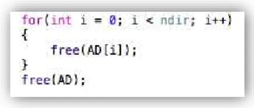
FIGURE 3.8:THE RELEASE OF THE MEMORY ALLOCATED FOR THE 𝐴_𝐷 MATRIX...40

FIGURE 3.9:FLOWCHART OF THE PLUGIN.THE COMPUTATION OF DKI QUANTITIES IS THE CENTRAL TASK OF THIS TOOL, AND IS REPEATED FOR EVERY SLICE IN THE SERIES. ...41

FIGURE 3.10:THIS PIECE OF CODE SHOWS THE FOR CYCLE RESPONSIBLE FOR ITERATING THROUGH THE IMAGES RESPECTING THE ORDER DESCRIBED IN MATRIX (90). ...42

FIGURE 3.11:THE DECLARATION OF POINTERS TO THE VOXEL CURRENTLY BEING PROCESSED, WHERE 𝑥 IS THE INDEX OF THE VOXEL BEING COMPUTED. ...42

FIGURE 3.12:FLOWCHART FOR THE DKICOMPUTATION FUNCTION ...43

FIGURE 3.13:THE INDEX OF THE DIFFUSION TENSOR ELEMENTS IN THE 𝑋_𝐷 ARRAY. ...44

FIGURE 3.14:THE POPULATION OF A IN THE ORDER DESCRIBED IN FIGURE 3.13. ...44

FIGURE 3.15:THE ORDERLY POPULATION OF THE EIGENVECTOR’S ARRAY...45

FIGURE 3.16:ONE OF THE CASES OF THE SWITCH STATEMENT DECLARED IN FIGURE 3.16.IN THIS CASE, THE SUM OF THE INDICES IS 2 WHICH OCCURS FOR BOTH 𝑊₀₀₀₂ AND 𝑊₀₀₁₁, THUS, THESE TWO CASES ARE DISTINGUISHED BY A SUBSEQUENT IF STATEMENT. ...46

FIGURE 3.17:FUNCTION FOR COMPUTING MK.VARIOUS IF STATEMENTS ARE IMPLEMENTED SO AS TO DEAL WITH ANY EVENTUAL SINGULARITIES IN COMPUTING 𝐹₁ AND 𝐹₂. ...48

FIGURE 3.18:PLUGIN INSTALLATION EXECUTABLE. ...49

FIGURE 4.1:MEAN DIFFUSION MAPS COMPUTED BY (A)DKI PLUGIN,(B)DKE SOFTWARE, USING THE CLLS-H AND CLLS-QP ALGORITHMS RESPECTIVELY. ...55

FIGURE 4.2:RADIAL DIFFUSION MAPS COMPUTED BY (A)DKI PLUGIN,(B)DKE SOFTWARE, USING THE CLLS-H AND CLLS-QP ALGORITHMS RESPECTIVELY. ...56

FIGURE 4.3:AXIAL DIFFUSION MAPS COMPUTED BY (A)DKI PLUGIN,(B)DKE SOFTWARE, USING THE CLLS-H AND CLLS-QP ALGORITHMS RESPECTIVELY. ...56

FIGURE 4.4:FRACTIONAL ANISOTROPY MAPS COMPUTED BY (A)DKI PLUGIN,(B)DKE SOFTWARE, USING THE CLLS-H AND CLLS-QP ALGORITHMS RESPECTIVELY. ...57

xxi

FIGURE 4.6:RADIAL KURTOSIS MAPS COMPUTED BY (A)DKI PLUGIN,(B)DKE SOFTWARE, USING THE CLLS-H AND

CLLS-QP ALGORITHMS RESPECTIVELY. ... 58 FIGURE 4.7:AXIAL KURTOSIS MAPS COMPUTED BY (A)DKI PLUGIN,(B)DKE SOFTWARE, USING THE CLLS-H AND

CLLS-QP ALGORITHMS RESPECTIVELY. ... 58 FIGURE 4.8:A LARGE ROI CONTAINING THE CENTRAL PART OF THE SLICE FOR THE MEAN KURTOSIS MAPS. ... 60 FIGURE 4.9:SMALL ROI IN MEAN DIFFUSION MAPS. ... 60 FIGURE 4.10:MAPS GENERATED BY THE PLUGIN,(A)MEAN DIFFUSION;(B)RADIAL DIFFUSON;(C)

AXIAL DIFFUSION;(D)FRACTIONAL ANISOTROPY. ... 62

FIGURE 4.11:MAPS GENERATED BY THE PLUGIN,(A)MEAN KURTOSIS;(B)RADIAL KURTOSIS;(C)AXIAL KURTOSIS. ... 63

FIGURE 4.12:AN EXAMPLE OF AN ACQUIRED IMAGE FOR (𝑏 = 0).AS PREDICTED, THE SEPARATION OF

THE SIGNAL FROM FAT, CREAM AND WATER IS VISIBLE DUE TO THE PREVIOUS HEATING

TREATMENT... 65 FIGURE 4.13:THE MEAN KURTOSIS MAPS FOR THE PHANTOM AND TWO ROIS,(A) WATER REGION AND (B) CREAM

xxiii

List of Tables

TABLE 2.1:MEAN SQUARED ERROR (MSE) AND STANDARD DEVIATION (SD) OF THE CORRECTED VOXEL

VALUES FOR THE ZEROAND ABSMETHODS. ... 52

TABLE 4.2:AVERAGE OF ALL MEAN VOXEL VALUES FOR THE ROIS DEFINED IN THE DKE GENERATED

MAPS AND THE MEAN SQUARED ERROR OF THE VALUES IN THE MAPS GENERATED BY THE

xxiv

Acronyms

AD Axial Diffusion

AK Axial Kurtosis

CLLS Constrained Linear Least Squares

CLLS-H Constrained Linear Least Squares – Heuristic

CLLS-QP Constrained Linear Least Squares – Quadratic Programming

DICOM Digital Imaging and Communications in Medicine

DKE Diffusional Kurtosis Estimator

DKI Diffusion Kurtosis Imaging

DTI Diffusion Tensor Imaging

DWI Diffusion Weighted Image

FA Fractional Anisotropy

IID Independent and Identically Distributed

MRI Magnetic Resonance Imaging

MD Mean Diffusion

MK Mean Kurtosis

MSE Mean Squared Error

xxv

PDF Probability Density Function

RD Radial Diffusion

RK Radial Kurtosis

SD Standard Deviation

1

1

Introduction

1.1

Motivation

Diffusion Kurtosis Imaging (DKI) is known to provide more accurate infor-mation on tissue microstructure than standard diffusion tensor imaging (DTI) and is applicable in situations where the latter is worthless, such as in investigat-ing abnormalities in grey matter and other tissues of isotropic nature [1].

Software for DKI computation has already been developed and made avail-able (diffusion kurtosis estimator (DKE) [31]), howbeit, it only works on win-dows platforms and its usage is not very straightforward. One setback of this software is that the gradient vectors, mandatory for DKI processing, are selected from a list that only comprises predefined SiemensTM _{protocols, as shown in}

fig-ure 1.1. This means, that, for a set of diffusion weighted images (DWIs) acquired from a different MRI manufacturer (e.g., PhilipsTM_{), the user must create the file}

with the gradient vectors. Additionally, DKE does not allow any type of image visualization and manipulation, which is very helpful in a medical environment. Moreover, it is not possible to choose which maps to generate, as this software computes maps for mean, radial and axial diffusion, fractional anisotropy and mean, radial and axial kurtoses metrics, increasing the processing time.

2 Figure 1.1: DKE graphical user interface.

All of this makes the development of an easy-learning and fast-processing DKI tool for medical usage of the utmost importance. This work attempts to answer this need by developing a tool for DKI computation in the form of a plugin for OsiriX.

The reason behind the choosing of OsiriX, was that it is an open source software dedicated to DICOM images ubiquitous in the medical world, with an architecture that permits an easy implementation of any developed tool in the form of a plugin. Also, all the required information for DKI computation is obtained directly from the image metadata, which excludes any need for additional inputs.

1.2

Objectives

The objective of this work is to answer the need for a fast and user-friendly tool

for DKI computation by developing a plugin for OsiriX capable of rapidly generate

maps for Mean Diffusion (MD), Radial Diffusion (RD), Axial Diffusion (AD),

Frac-tional Anisotropy (FA), Mean Kurtosis (MK), Radial Kurtosis (RK) and Axial Kurtosis

3

One of the main goals for this tool is to assure its ergonomic usage as the

user will only be required to select which maps are to be computed and to define

a threshold for voxel computation and an additional control variable. No

addi-tional inputs are needed since all the information required by the program is

assessed through the Diffusion Weighted Images (DWIs) set’s metadata given

that it is complete.

1.3

State of the art

Diffusion has been measured through spin echoes since the 1950. And, in

the 1980s, a combination with magnetic resonance imaging (MRI) emerged which

allowed for a better understanding of diffusion processes in human brain. This

technique only described diffusion as a scalar constant, which was not accurate

in assessing the heterogeneities of biological tissue. As a result, in 1994, Basser et

al. proposed a new MRI modality, which consisted on, within a voxel, estimating

a symmetric, positive definite 3x3 tensor, which would provide some insight on

the diffusion on that very voxel [2]. This technique is commonly referred to as

diffusion tensor imaging (DTI) and has been widely used ever since. By analysing

the anisotropic displacement of water in several voxels, DTI was shown to

pro-vide useful information such as fibre tract orientation and mean particle

displace-ments [2].

One key aspect of diffusion tensor imaging is the assumption that water

displacement follows a gaussian probability distribution function (PDF), which

only holds for simple homogeneous liquids (e.g., a glass of water) [3]. This

as-sumption is translated into a monoexponential dependency of the

diffusion-weighted (DW) signal on b-value. However, the relationship between the

diffu-sion weighted signal and the b-value in neural tissues is known to be

non-mo-noexponential [4]. The reason behind this is that in biological tissues, the

4

gaussian form. Therefore, DTI is not an accurate technique in describing water

diffusion [5].

Before attempting to characterize water diffusion in biological tissues, one

must have an underlying model to describe the mechanisms behind this process.

However, an accurate modelling of water diffusion in non-homogeneous

envi-ronments (more specifically in biological tissues) is extremely complex. Many

models have been developed to characterize water diffusion in brain. These

in-clude the multicompartment model which is the simplest and most applied one

[6], the Kärger model [7], the statistical diffusion model [8], the generalized

dif-fusion tensors [9] and one-dimensional model with barriers [10]. These models

serve as a basis for interpretation of the quantities measured in diffusion MRI

techniques, when in fact, the actual calculated values do not depend on the

adopted model.

Although it is possible to get the full PDF for water diffusion rather than

just the excess kurtosis by means of q-space imaging using very well-defined

im-aging methods [11], this level of accuracy is very demanding in hardware and

requires large b-values and a strong gradient. Because of this, it is very difficult

to fit such protocols in a medical environment [6]. DKI sidesteps these costly

re-quirements and emerges as a refined diffusion MRI technique by introducing a

dimensionless metric known as diffusional kurtosis, the 4th central moment of

the diffusion distribution. And, by doing so, DKI quantifies the extent to which

water diffusion is non-Gaussian. The higher the diffusion kurtosis, the more the

restrictions are imposed by the environment.

Since its introduction, and because DKI yields not only conventional

diffu-sion information but also the diffudiffu-sional kurtosis, it has been successful in several

studies where conventional MRI was only partially succeeding. For instance, in

an attempt to identify biological mechanisms underlying ischemia by analysis of

diffusion in white matter (WM), DKI throve as the kurtosis maps exhibited

het-erogeneities in ischemic lesions which were not present on the diffusion maps

5

pathologies such as Alzheimer’s disease [13], attention-deficit hyperactivity

dis-order (ADHD) [14] and schizophrenia [15].

The DKI model is parameterized by the diffusion and kurtosis tensors (𝑫 and 𝑲). The estimation of these tensors for each and every voxel is the core of

DKI computing as all the important metrics in DKI analysis are derived from

them.

There are several ways to estimate the diffusion and kurtosis tensors.

Meth-ods such as unconstrained nonlinear least squares (UNLS) and unconstrained

linear least squares (ULLS) have been used to estimate 𝑫 and 𝑲 and were shown

not to provide satisfactory tensor estimates. And even after some adjustments,

the algorithms are not viable when compared to constrained linear least squares

(CLLS) formulations [16].

The CLLS formulation is simply a casting of the tensor estimation problem

as linear least squares with linear constrains safeguarding the physical and

bio-logical meaning of directional diffusivities and kurtoses. Tabesh et al., 2011,

pro-posed two algorithms for solving the CLLS formulation for 𝑫 and 𝑲 estimation,

the quadratic programming (CLLS-QP) approach and the heuristic (CLLS-H)

ap-proach. Both these algorithms gave more reliable estimations of the tensors, with

the CLLS-QP providing the exact solution for the estimation problem a higher

computational cost and the CLLS-H yielding an approximate solution at a lower

processing time.

The CLLS-QP algorithm is implemented in DKE, which, as mentioned

be-fore, is a software for processing DKI datasets. This software is currently

sup-ported on 32 and 64-bit Windows platforms. It consists on a graphical user

inter-face (GUI) and a set of comand-line based programs. The software generates

maps for standard DTI quantities (MD, AD, RD and FA) as well as for DKI

met-rics (MK, AK, RK). It accepts both DICOM and NIfTI formats and the user may

choose the algorithm for 𝑫 and 𝑲 estimation from: constrained linear weighted,

7

2

Theoretical Background

2.1

Diffusion MRI

The diffusion of a water molecule through a given medium can be

charac-terized as a Brownian random process, meaning that the motion of the particle is

the result of a large number of collisions with the surrounding particles. These

collisions are independent and identically distributed (i.i.d.), hence, as stated by

the central limit theorem, the sum of many i.i.d variables with finite mean and

standard deviation results in a normal distribution, the probability that a particle

undergoes a vectorial displacement 𝒓 over a time interval 𝒕 is given by a Gaussian

distribution [17]. The describing of water diffusion in biological tissues by a

Gaussian PDF is the core of diffusion tensor imaging. However, as mentioned

before, this only holds for homogeneous liquids, whereas for biological tissues,

the restrictions imposed by tissue microstructure deviate the PDF from a

Gauss-ian form.

8

Diffusion Kurtosis Imaging (DKI) tackles the problem of non-gaussianity

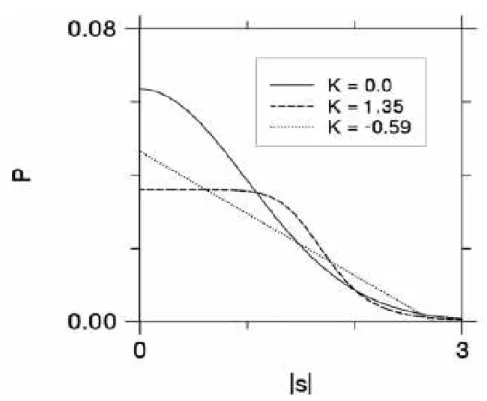
as-sumed in diffusion tensor imaging (DTI) by quantifying the kurtosis of the

diffu-sion PDF. Figure 2.1 shows three different PDFs with identical diffusion coeffi-cients but different values of kurtosis, which proves that the diffusion coefficient

alone does not provide enough insight on the motion of water molecules.

Figure 2.1: Three isotropic diffusion displacement probability distributions. The corresponding diffusion coefficients are identical, but the values for diffusional

kurto-sis are different. The solid curve with 𝑲 = 𝟎 is the Gaussian form. Taken from [1].

2.2

Definition of Kurtosis

9 𝛽2 = 𝐸(𝑋 − 𝜇)

4 (𝐸(𝑋 − 𝜇)2₎2 =

𝜇4

𝜎4 (1)

where 𝐸 is the expectation operator, 𝜇 is the mean, 𝜇₄ is the fourth moment about the mean and 𝜎 the standard deviation.

A Gaussian distribution has a kurtosis of 3. Consequently, 𝛽₂− 3 is conven-iently used so that the reference normal distribution has a kurtosis of zero. The minimum theoretical value for kurtosis is therefore −2.

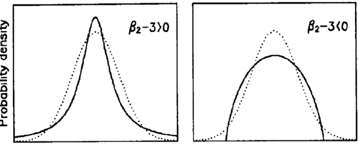
Figure 2.2 illustrates two distributions, on the left a distribution with posi-tive kurtosis (leptokurtic) and on the right, a distribution with negaposi-tive kurtosis (platykurtic). It is clear that distributions with negative kurtosis are flatter and have lighter tails, whereas distributions with positive kurtosis have a higher peak and heavier tails.

Figure 2.2: An illustration of two distributions with different kurtosis. The dot-ted lines show Gaussian distributions, the solid lines show distributions with positive

kurtosis (left panel) and negative kurtosis (right panel). Taken from [18].

10

2.3

Modelling water diffusion

Considering 𝑃(𝒓, 𝑡) as a PDF for water diffusion, with 𝒓being the vectorial

displacement of a given molecule over a time interval 𝒕. One may average an arbitary function 𝐴(𝒓) over that very PDF as follows

⟨𝐴(𝒓)⟩ = ∫ 𝑑3_{𝒓 𝑃(𝒓, 𝑡)𝐴(𝒓) (2)}

The diffusion coefficient of the water molecule in a direction 𝒏, and

assum-ing |𝒏| = 1, is given by

𝐷(𝒏) =_2𝑡1 ⟨(𝒓 · 𝒏)2_{⟩ (3)}

The diffusional kurtosis is defined by taking equation (1) and subtracting 3

in order to assure a kurtosis of 0 for a Gaussian diffusion.

𝐾(𝒏) =_{⟨(𝒓 · 𝒏)}⟨(𝒓 · 𝒏)₂4_⟩⟩₂− 3 (4)

Both these metrics are defined as tensors in order to account for the

aniso-tropic characteristics of the medium and quantify the directionality of the

diffu-sion process. The diffudiffu-sion tensor 𝑫 is defined as

𝐷𝑖𝑗= _2𝑡1 ⟨𝑟𝑖𝑟𝑗⟩ (5)

and the coefficients of the kurtosis tensor 𝑲 as

𝑊𝑖𝑗𝑘𝑙 =_{⟨𝒓 ·𝒓⟩}9 ₂(⟨𝑟𝑖𝑟𝑗𝑟𝑘𝑟𝑙⟩ − ⟨𝑟𝑖𝑟𝑗⟩⟨𝑟𝑘𝑟𝑙⟩ − ⟨𝑟𝑙𝑟𝑘⟩⟨𝑟𝑗𝑟𝑖⟩ − ⟨𝑟𝑖𝑟𝑙⟩⟨𝑟𝑗𝑟𝑘⟩) (6)

with 𝑟_𝑖 being the i-th component of the displacement vector 𝒓.

These two tensors allow the calculation of the diffusion coefficient and

dif-fusional kurtosis in a given direction as follows

𝐷(𝒏) = ∑ ∑ 𝑛𝑖𝑛𝑗𝐷𝑖𝑗 3

𝑗=1 3

𝑖=1

11

and

𝐾(𝒏) = 𝐷 2

[𝐷(𝒏)]2∑ ∑ ∑ ∑ 𝑛𝑖𝑛𝑗𝑛𝑘𝑛𝑙𝑊𝑖𝑗𝑘𝑙 3

𝑙=1 3

𝑘=1 3

𝑗=1 3

𝑖=1

(8)

The components of 𝑫 may be used to describe the diffusion geometrically.

An isotropic diffusion is represented by a 3D sphere as there is no preferential

direction to the diffusion process whereas, for anisotropic diffusion the 3D

rep-resentative is an ellipsoid. A much more complex structure is needed to describe

the diffusional kurtosis due to 𝑲being a 4-th order tensor. Figure 2.4 illustrates the diffusion ellipsoid for an anisotropic environment (e.g. white matter axons)

and attempts to represent the diffusional kurtosis as a pancake-like ellipsoid.

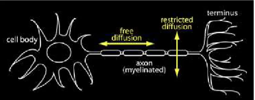
Since diffusion is most freely along the fibres, as illustrated in figure 2.3, the

dif-fusion ellipsoid is wider on that direction while the kurtosis is very small. On the

other hand, in the perpendicular direction, fibre barriers prevent a free diffusion

deviating the diffusion PDF from a gaussian behaviour. And since kurtosis

quan-tifies this deviation, the kurtosis ellipsoid is wider along that very direction.

12

Figure 2.4: An illustration of the diffusion and kurtosis distribution in the 3D system defined by diffusion eigenvectors (𝛌_𝟏, 𝛌_𝟐, 𝛌_𝟑). The diffusion distribution is an

ellipsoid (blue) with the principle direction pointing at 𝛌_𝟏. The kurtosis distribution, from a simplified point of view, is like a pancake (yellow) with higher kurtosis along radial direction of the diffusion ellipsoid, indicating restricted diffusion. Taken from

[5].

Despite being model-independent and therefore physically well-defined,

both the diffusion coefficient and the diffusional kurtosis demand an underlying

model for water diffusion in order to understand the information they hold

re-garding tissue structure.

The simplest model is the multiple compartment model with no water

ex-change. This model attempts to characterize water diffusion in brain by

consid-ering multiple compartments that represent diverse microstructures such as

ex-tracellular and inex-tracellular spaces and white matter tracts. Although there are

models that cover the flow of water from one compartment to the other such as

the two-comparment model with water exchange, also reffered to as the Kärger

model [7], and the one-dimensional model with barriers [10], this work will adopt

13

2.3.1

Multiple compartment model

The PDF that describes the Gaussian diffusion of a water molecule within a

single compartment is given by

𝑃(𝑟, 𝑡) = _{(4𝜋𝑡)3/2}1_|𝐷|1/2𝑒−𝒓𝑇𝑫−14𝑡𝑟 ₍₉₎

with 𝑫representing the diffusion tensor.

If one considers 𝑁 compartments, equation (9) is generalized to

𝑃(𝑟, 𝑡) = ∑ 𝑓𝑚 𝑁

𝑚=1

1

(4𝜋𝑡)3/2_|𝐷(𝑚)_|1/2𝑒−𝒓

𝑇_𝑫(𝒎)−1𝑟

4𝑡 (10)

with 𝐷(𝑚) being diffusion tensor and 𝑓_𝑚 the water fraction for the m-th compart-ment [19].

Note that the sum of all water fractions must add up to 1.

∑ 𝑓𝑚 𝑁

𝑚=1

= 1 (11)

The total diffusion is the weighted sum of the diffusion coefficients of all

the 𝑁 compartments.

𝐷(𝒏) = ∑ 𝑓𝑚𝐷(𝑚)(𝒏) 𝑁

𝑚=1

(12)

As for the diffusional kurtosis, equations (7), (8) and (10) give

𝐾(𝒏) = 3_[𝐷(𝒏)]𝛿2𝐷(𝒏)₂ (13)

with the term 𝛿2𝐷(𝒏) being the variance of the diffusion coefficient given by

𝛿2_{𝐷(𝒏) = ∑ 𝑓}

𝑚{[𝐷(𝑚)(𝒏) − 𝐷(𝒏)]2} 𝑁

𝑚=1

14

This way, the multiple compartment model, in its attempt to explain the

meaning of diffusional kurtosis, gives a qualitative definition for this metric as

stated in [6]: “kurtosis is a measure of the heterogeneity of the diffusion environment”.

2.4

MRI signal

Having discussed the theory behind diffusion and kurtosis, the respective

tensors and the adopted multi compartment model for water diffusion in brain,

it is necessary to elaborate on the relationship to the measured MRI signal.

An example of a very accurate yet very demanding, not only in terms of

hardware but also because of the long acquisition times, technique for

character-izing water diffusion in brain is the q-space approach. It essentially fully

deter-mines the PDF which makes it possible to calculate the kurtosis directly from

equation (4). However, this technique is not easily incorporated into clinical

im-aging protocols, as the b-values are very large. Another powerful and demanding

technique is diffusion spectrum imaging (DSI), which is a 6D MRI technique

sim-ilar to q-space. It also uses large b-values (e.g. 𝑏 = 17000 s/mm2) and long acqui-sition times (e.g. 25 min.) [11].

Diffusion kurtosis imaging, on the other hand, is a less demanding

tech-nique that consists on an extension of traditional diffusion tensor imaging.

2.4.1

DKI as an extension of DTI

The key factor in DTI is that the diffusion process produces an attenuation

of the measured echo signal. This attenuation, given by equation (16) is a function

15 𝑏 = 𝛾2_𝐺2_𝛿2_{(∆ −}𝛿

3) (15)

with 𝛾 being the proton gyromagnetic ratio, 𝐺 is the amplitude of the diffusion

sensitizing magnetic field gradient pulses, 𝛿 the duration of the gradient pulses and ∆ the time interval between centers of gradient pulses. The b-value is altered

by varying 𝐺.

The dependence of the diffusion-weighted signal on the b-value is given by

ln [𝑆(𝑏)] = ln [𝑆0] − 𝑏𝐷𝑎𝑝𝑝+ 𝑂(𝑏2) (16)

where 𝑆(𝑏) and 𝑆₀ are echo magnitudes of the diffusion weighted and non-diffu-sion-weighted (𝑏 = 0) signals respectively [20], and 𝐷_𝑎𝑝𝑝 is the ‘apparent’ diffu-sion coefficient which, for the non-exchanging multiple compartment described above, is essentially the true diffusion coefficient 𝐷 for a diffusion time 𝑡 = ∆ with an infinitesimal pulse duration (𝛿 → 0) [6]. Moreover, if the 𝑂(𝑏2) term is made negligible by using sufficiently small b-values, the following approxima-tion is valid

ln[𝑆(𝑏)] ≈ ln[𝑆0] − 𝑏𝐷(𝑡) (17)

This equation would be exact should the diffusion’s PDF be purely

Gauss-ian, and it could be rewritten as

𝑆(𝑏) = 𝑆0𝑒−𝑏𝐷 (18)

Since equation (17) has two unknowns, at least two b-values are needed in

order to estimate 𝐷. If exactly two b-values are used, the following closed form

solution arises

𝐷 ≈ _𝑏 1 2− 𝑏1ln [

𝑆(𝑏1)

𝑆(𝑏2)] (19)

DKI is built upon DTI by considering the contribution of the 𝑂(𝑏2) term in equation (16) which concerns the diffusional kurtosis. This translates into the

fol-lowing cumulant expansion [21]

16

with 𝐾_𝑎𝑝𝑝 being the ‘apparent’ diffusional kurtosis which, as mentioned above, for the adopted multiple compartment model, is the true diffusional kurtosis 𝐾.

In addition to this and if, once again, the chosen b-values are small enough

to assure that the 𝑂(𝑏3) term is negligible, equation (16) may be rewritten as

ln[𝑆(𝑏)] = ln[𝑆0] − 𝑏𝐷 +1_{6 𝑏}2𝐷2𝐾 (21)

or

𝑆(𝑏) = 𝑆0𝑒−𝑏𝐷+16𝑏

2_𝐷2_{𝐾 (22)}

Similarly to DTI, in DKI the range of b-values must be so that precision is

assured whilst maintaining the 𝑂(𝑏3) term meaningless. However, the cumulant expansion of the diffusion-weighted signal allows for higher values.

The expansion of equation (16) adds a new unknown to the estimation

prob-lem. Thus, to reach a closed-form solution, there must be at least three b-values.

Should that be the case, the following expressions are applicable

𝐷 ≈ (𝑏3+ 𝑏1)𝐷(12)_(𝑏 − (𝑏2+ 𝑏1)𝐷(13)

3− 𝑏2) (23)

and

𝐾 ≈ 6𝐷_(𝑏(12)− 𝐷(13)

3− 𝑏2)𝐷2 (24)

with

𝐷(1𝑖)=𝑙𝑛 [𝑆(𝑏 1) 𝑆(𝑏𝑖)] (𝑏𝑖− 𝑏1)

(25)

2.4.1.1

b

_{-value range}

To guarantee accurate parameter estimation, an upper bound for the b

-value must be set for DTI as well as for DKI. The DKI model is the better

17

to the consideration of the 𝑂(𝑏2) term whose contributions grow with increasing b-values.

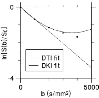
Figure 2.5:Comparison of DTI and DKI fitting models. For DTI, the logarithm of diffusion-weighted signal intensity (circles) as a function of the b-value is fit, for small b-values, to a straight line. In brain, this fit is often based on the signal for b = 0 and b = 1000 s/mm2. For DKI, the logarithm of the signal intensity is fit, for small b-values, to a parabola. In brain, this fit may be based on the signal for b = 0, b = 1000, and b = 2000

s/mm2. Taken from [6].

For DTI, the maximum b-value that assures precision whilst guaranteeing

small contributions from the 𝑂(𝑏2) term is about1000 s/mm2[6].

As for DKI, by assuming 𝑆(𝑏) as a monotonically decreasing function of b, which is empirically true for biological tissues [6], the maximum allowed value

for b that assures this is calculated as

𝜕

𝜕𝑏(−𝑏𝐷 + 1

6 𝑏2𝐷2𝐾) ≤ 0 (26)

18

𝑏 <_𝐷𝐾3 (27)

Typical values in brain are around 𝐷 ≈ 1𝜇𝑚2/𝑚𝑠 and 𝐾 ≈ 1, thus, the max-imum b-value should be somewhere around 3000 s/mm2 [19].

2.5

Algorithm for DKI computation

There are several ways to estimate the diffusion and kurtosis tensors 𝑫and

𝑲. Methods such as unconstrained nonlinear least squares (UNLS) and uncon-strained linear least squares (ULLS) have been used and were shown not to pro-vide good tensor estimations [16].

In this work, the tensor estimation problem will be cast as a linear least squares with linear constrains safeguarding the physical and biological meaning of directional diffusivities and kurtoses. The formulation of the problem is pre-sented ahead.

2.5.1

Formulation

The diffusion-weighted signal for a given direction 𝒏 and b-value 𝑏 given by equation (21) may be rewritten using equations (7) and (8) as

ln [𝑆(𝒏, 𝑏)_𝑆

0 ] = − 𝑏 ∑ ∑ 𝑛𝑖𝑛𝑗𝐷𝑖𝑗 3

𝑗=1 3

𝑖=1

+1_{6 𝑏}2_𝐷2_{∑ ∑ ∑ ∑ 𝑛}

𝑖𝑛𝑗𝑛𝑘𝑛𝑙𝑊𝑖𝑗𝑘𝑙 3 𝑙=1 3 𝑘=1 3 𝑗=1 3 𝑖=1 (28)

Note that both 𝐷_𝑖𝑗 and 𝑊_{𝑖𝑗𝑘𝑙} are symmetric as to the interchangeability of its indices, thus, the diffusion tensor 𝑫 has 6 independent degrees of freedom, whereas the kurtosis tensor 𝑾 has 15 [19]. Hence, there are 6 + 15 = 21 param-eters to be estimated.

The set of linear constraints is given by the following equations

19

𝐾𝑚𝑎𝑥(𝒏) ≥ 𝐾(𝒏) ≥ 𝐾𝑚𝑖𝑛 (30)

where 𝐾_𝑚𝑎𝑥 denotes the maximum allowed value for kurtosis and may be ex-pressed as

𝐾𝑚𝑎𝑥(𝒏) =_𝑏 𝐶

𝑚𝑎𝑥𝐷( 𝒏) , 3 ≥ 𝐶 ≥ 0 (31)

by rearranging equation (27). The variation on 𝐶 regulates the level of restriction applied to the kurtosis values, nevertheless, 𝐶 is usually set to 3 so as to be con-sistent with equation (27).

As for the minimum value for kurtosis (𝐾_𝑚𝑖𝑛), although its theoretical min-imum is −2, it is normally set to zero because, as predicted by equation (13), the multiple compartment diffusion model suggests a super-Gaussian displacement distribution, meaning 𝐾 ≥ 0. Also, all the empirical evidence in brain gathered so far never yielded negative kurtosis values [16].

Simply put, the estimation problem consists in finding 𝑫 and 𝑾 that not only assure the exactness of equation (28) but also meet the constraints in equa-tions (29) and (30).

All in all, the problem is

Minimize ‖𝑨𝑿 − 𝑩‖2

(32) such that 𝑪𝑿 ≤ 𝒅,

with

𝑿 = [𝐷11, 𝐷22, 𝐷33, 𝐷12, 𝐷13, 𝐷23, 𝐷2𝑊1111, … , 𝐷2𝑊1122, … , 𝐷2𝑊1233] 𝑇

(33)

being a vector with the 21 unknown parameters of 𝑫and 𝑾, 𝑨a matrix defined as

𝑨 =

[

−𝑏1𝐴𝐷(1) 1_{6 𝑏}12𝐴𝐾(1)

⋮ ⋮

−𝑏𝑀𝐴𝐷(𝑀) 1_{6 𝑏}𝑀2𝐴𝐾(𝑀)_]

(34)

20 [𝐴𝐷(𝑖)]_𝑘 = [(𝑛𝑘1(𝑖))2, (𝑛𝑘2(𝑖))2, (𝑛𝑘3(𝑖))2, 𝑛𝑘1(𝑖)𝑛𝑘2(𝑖), 𝑛𝑘1(𝑖)𝑛𝑘3(𝑖), 𝑛𝑘2(𝑖)𝑛𝑘3(𝑖)] (35)

and

[𝐴𝐾(𝑖)]_𝑘 = [(𝑛𝑘1(𝑖)) 4

, (𝑛_𝑘2(𝑖))4, (𝑛_𝑘3(𝑖))4, 4(𝑛_𝑘1(𝑖))3𝑛(𝑖)_𝑘2, 4(𝑛_𝑘1(𝑖))3𝑛_𝑘3(𝑖), 4(𝑛_𝑘2(𝑖))3𝑛_𝑘1(𝑖),

4(𝑛_𝑘2(𝑖))3𝑛_𝑘3(𝑖), 4(𝑛_𝑘3(𝑖))3𝑛_𝑘1(𝑖), 4(𝑛_𝑘3(𝑖))3𝑛_𝑘2(𝑖), 6(𝑛_𝑘1(𝑖))2(𝑛_𝑘2(𝑖))2, 6(𝑛_𝑘1(𝑖))2(𝑛_𝑘3(𝑖))2,

6(𝑛_𝑘2(𝑖))2(𝑛_𝑘3(𝑖))2, 12𝑛_𝑘2(𝑖)𝑛_𝑘3(𝑖)(𝑛_𝑘1(𝑖))2, 12𝑛_𝑘1(𝑖)𝑛_𝑘3(𝑖)(𝑛_𝑘2(𝑖))2, 12𝑛_𝑘1(𝑖)𝑛_𝑘2(𝑖)(𝑛_𝑘3(𝑖))2]

(36)

respectively, with 𝑛_𝑘𝑗(𝑖) being the j-th component of the k-th gradient direction for the i-th b-value.

Additionally, the vector 𝑩is expressed as

𝑩 = [ln (𝑆(𝒏_𝑆𝑘(𝑖), 𝑏𝑖)

0 ) … ln (

𝑆(𝒏_𝑘(𝑀), 𝑏𝑀) 𝑆0 )]

𝑇

(37)

where 𝑆(𝒏_𝑘(𝑖), 𝑏_𝑖) is the signal intensity for the k-th direction of the i-th b-value.

The linear constraints are described by matrix 𝑪 which is built as follows

𝑪 = [

−𝐴𝐷 0

0 −𝐴𝐾

−_𝑏𝐶

𝑚𝑎𝑥𝐴𝐷 −𝐴𝐾]

(38)

where

𝐴𝐷 = [ 𝐴_𝐷(1)

⋮ 𝐴_𝐷(𝑀)

] (39)

and

𝐴𝐾 = [ 𝐴_𝐾(1)

⋮ 𝐴_𝐾(𝑀)

] (40)

Finally, vector 𝒅 is given by

𝒅 = [𝟎 𝐾𝑚𝑖𝑛𝐷(𝒏1(1))2… 𝐾𝑚𝑖𝑛𝐷(𝒏𝑁(1)) 2

… 𝐾𝑚𝑖𝑛𝐷(𝒏1(𝑀)) 2

… 𝐾𝑚𝑖𝑛𝐷(𝒏𝑁(𝑀)) 2

21

where 𝟎is a one-dimensional vector with 𝑁 elements.

2.5.2

Solution

The exact solution to the described problem is attainable via quadratic pro-gramming using standard algorithms such as active set and interior-point [16]. However, in this work, the estimation of 𝑫and 𝑲 will be executed using a heu-ristic constrained linear least squares algorithm (CLLS-H) described ahead.

Firstly, unlike the quadratic programming methods that not only allow any number of b-values but also accept different gradient directions for each of the b -values, the CLLS-H algorithm uses exactly two nonzero b-values and equal gra-dient directions for both of them, meaning

𝑵(1) _{= 𝑵}(2)_{= {𝒏}

1, … , 𝒏𝑁} (42)

where 𝑁 is the number of gradient directions. This way, there are 2𝑵 + 1 images for every slice, where the term +1 regards the 𝑏₀ image.

The algorithm starts by estimating 𝐷(𝒏_𝑖) and 𝐾(𝒏_𝑖) along each direction using equations (23) and (24) and assuming 𝑏₁to be the zero b-value and 𝑏₃ to-gether with 𝑏₂ to be the nonzero b-values now denoted as 𝑏₂ and 𝑏₁respectively. Thus we have

𝐷𝑖 =𝑏2𝐷𝑖 (1)_{− 𝑏}

1𝐷𝑖(2) 𝑏2 − 𝑏1

(43)

𝐾𝑖 = 𝐷𝑖 (1)_{− 𝐷}

𝑖(2) (𝑏2− 𝑏1)𝐷(𝑛𝑖)2

(44)

with 𝐷_𝑖(1) and 𝐷_𝑖(2) calculated from equation (25).

The next step is to constrain 𝐷_𝑖 using a the following set of rules

If 𝐷_𝑖 ≤ 0, set 𝐷_𝑖= 0.

Else, if 𝐷_𝑖(1) < 0, set 𝐷_𝑖 = 0.

22

Else, if 𝐷_𝑖 > 0 and 𝐾_𝑖< 𝐾_𝑚𝑖𝑛, If 𝐾_𝑚𝑖𝑛 = 0, set 𝐷_𝑖 = 𝐷_𝑖(1).

Else, set 𝐷_𝑖= 1_𝑥[√1 −2₃𝐾_𝑚𝑖𝑛𝑏₁𝐷_𝑖(1)− 1].

Else, if 𝐷_𝑖 > 0 and 𝐾_𝑖> 𝐾_𝑚𝑎𝑥 (𝐾_{𝑚𝑎𝑥𝑖} = 𝐾_𝑚𝑎𝑥(𝑛_𝑖)) set 𝐷_𝑖 = 𝐷𝑖

(1)

1−𝐶_{6𝑏𝑚𝑎𝑥}𝑏1

where 𝑏_𝑚𝑎𝑥 is the largest b-value used. The 𝑫tensor may now be estimated as

𝑋̂𝐷 = 𝐴𝐷+𝑏𝐷 (46)

where 𝑋̂_𝐷 is the unconstrained estimate of the 6 independent indices of the diffusion tensor 𝑫,

𝑋𝐷 = [𝐷11, 𝐷22, 𝐷33, 𝐷12, 𝐷13, 𝐷23]𝑇 (47)

and

𝑏𝐷 = [𝐷1, … , 𝐷𝑁] (48)

The 𝐴_𝐷+ term represents the pseudoinverse of the 𝐴_𝐷 matrix defined in equa-tions (35) and (39). This pseudoinverse matrix 𝐴_𝐷+ is simply a generalization of the inverse matrix 𝐴_𝐷−1 which is normally used to solve systems of linear equa-tions by the least squares method. This matrix is necessary when 𝐴_𝐷 is not a square, invertible matrix, which is the case.

Following this step, the 𝐷_𝑖 set is re-estimated using the following relation-ship

𝑏_𝐷(𝑅) = 𝐴𝐷𝑋̂𝐷 (49)

This re-estimation as a noise removal effect on the 𝐷_𝑖 set by assuring its con-sistency with 𝑋̂_𝐷 [16].

At this point, we can re-estimate 𝐾_𝑖

𝐾_𝑖(𝑅) = {6

𝐷_𝑖(𝑅)− 𝐷_𝑖(2) 𝑏2(𝐷𝑖(𝑅))

2 𝑖𝑓 𝐷𝑖(𝑅) > 0

0 𝑜𝑡ℎ𝑒𝑟𝑤𝑖𝑠𝑒

(50)

23

If 𝐾_𝑖(𝑅) > 𝐾_𝑚𝑎𝑥(𝑅) , set 𝐾_𝑖(𝑅) = 𝐾_𝑚𝑎𝑥(𝑅) .

(51) If 𝐾_𝑖(𝑅) < 𝐾_𝑚𝑖𝑛, set 𝐾_𝑖(𝑅) = 𝐾_𝑚𝑖𝑛.

The previous steps assure that the calculated diffusion coefficients are pos-itive and the diffusional kurtoses lie within a physically acceptable range. If the calculated value for the diffusion coefficient is negative, that very coefficient as well as the kurtosis are automatically set to zero. Consequently, the effects of noise, motion and imaging artifacts that cause the misestimation are reduced con-siderably [6].

Lastly, the kurtosis tensor 𝑲is estimated as

𝑋̂𝐾 = 1 𝐷2𝐴𝐾

+_𝑏

𝐾 (52)

where 𝑋̂_𝐾 denotes the ULLS estimate of 𝑲, the vector 𝑏_𝐾 is acquired as fol-lows, from the re-estimated the 𝐾_𝑖 values

𝑏𝐾 = [(𝐷𝑖(𝑅)) 2

𝐾₁(𝑅), … , (𝐷_𝑁(𝑅))2𝐾_𝑁(𝑅)]𝑇 (53)

and, similarly to 𝐴_𝐷+, 𝐴_𝐾+ represents the pseudoinverse of the matrix 𝐴_𝐾, which is described by equations (36) and (40).

2.6

Standard DTI metrics

Having estimated the diffusion and kurtosis tensors, the requested metrics may be computed. To do so, the coordinate system of each voxel is set to a refer-ence frame that diagonalizes 𝑫. The ensuing step is to get the diffusion tensor eigenvalues 𝜆₁, 𝜆₂, and 𝜆₃, which are ordered as

𝜆1 > 𝜆2 > 𝜆3. (54)

24

2.6.1

Mean diffusion (MD)

Mean diffusion, calculated as (55), represents the overall displacement of the water molecules and is independent of the orientation of the reference frame [22].

𝑀𝐷 =λ1+ λ₃2+ λ3 (55)

2.6.2

Axial diffusion (AD)

Axial diffusion (𝐷_||) measures the diffusion along the main axis of the diffu-sion ellipsoid and is therefore given by

𝐷|| = λ1 (56)

Axial diffusion is of the utmost importance because, for example, in white matter, as the main axis of the diffusion ellipsoid is aligned with the fibre direc-tion, the axial diffusion is simply the diffusion value along the fibres. This way, it is believed that it may shed a light on axonal integrity [23].

2.6.3

Radial diffusion (RD)

Radial diffusion (𝐷_┴) represents the diffusion along the axis orthogonal to the main axis of the ellipsoid, thus, it is calculated as the average between λ₂ and

λ3, and, following the previous example, in white matter, it quantifies the diffu-sion across the fibers and may help to study myelin integrity [23].

𝐷┴ = λ2+ λ₂ 3 (57)

2.6.4 Fractional anisotropy (FA)

25 𝐹𝐴 = √3_{2 √}(λ1− 𝑀𝐷)2+ (λ2− 𝑀𝐷)2+ (λ3 − 𝑀𝐷)2

λ12+ λ22+ λ32

(58)

2.7

DKI metrics

As for DKI quantities, some more intricate calculations are demanded.

2.7.1 Mean kurtosis (MK)

Mean kurtosis, similarly to mean diffusion, is the overall kurtosis in all di-rections of the diffusion ellipsoid, and is calculated as

𝑀𝐾 = 𝐹1(𝜆1, 𝜆2, 𝜆3)𝑊̃1111+ 𝐹1(𝜆2, 𝜆1, 𝜆3)𝑊̃2222+ 𝐹1(𝜆3, 𝜆2, 𝜆1)𝑊̃3333 + 𝐹2(𝜆1, 𝜆2, 𝜆3)𝑊̃2233+ 𝐹2(𝜆2, 𝜆1, 𝜆3)𝑊̃1133

+ 𝐹2(𝜆3, 𝜆2, 𝜆1)𝑊̃1122

(59)

where 𝑊̃_{𝑖𝑗𝑘𝑙} are the components of the kurtosis tensor in the reference frame that diagonalizes the diffusion tensor, and are calculated as follows

𝑊̃𝑖𝑗𝑘𝑙= ∑ ∑ ∑ ∑ 𝑒𝑖′𝑖𝑒𝑗′𝑗𝑒𝑘′𝑘𝑒𝑙′𝑙𝑊𝑖′𝑗′𝑘′𝑙′ 3 𝑙′=1 3 𝑘′=1 3 𝑗′=1 3 𝑖′=1 (60)

with 𝑒_𝑖𝑗 being the i-th component of the eigenvector corresponding to 𝜆_𝑗, and

𝑊𝑖′𝑗′𝑘′𝑙′ the component of 𝑲 for indices (𝑖, 𝑗, 𝑘, 𝑙) [24].

The functions 𝐹₁ and 𝐹₂ are given by

𝐹1(𝜆1, 𝜆2, 𝜆3) = (λ1+ λ2+ λ3) 2 18(λ1− λ2)(λ1− λ3)[

√λ2λ3 λ1 𝑅𝐹(

λ1 λ2,

λ1 λ3, 1)

+3λ1 2_{− λ}

1λ2 − λ1λ3 − λ2λ3 3λ1√λ2λ3 𝑅𝐷

(λ1 λ2,

λ1

λ3, 1) − 1]

26 𝐹2(𝜆1, 𝜆2, 𝜆3) =(λ1+ λ2+ λ3)

2 3(λ2 − λ3)2 [

λ2 + λ3 √λ2λ3 𝑅𝐹(

λ1 λ2,

λ1 λ3, 1)

+2λ1− λ2− λ3 3√λ2λ3 𝑅𝐷(

λ1 λ2,

λ1

λ3, 1) − 2]

(62)

where 𝑅_𝐹 and 𝑅_𝐷 are Carlson’s elliptic integrals [25], which are defined as

𝑅𝐹(𝑥, 𝑦, 𝑧) =1₂∫ [(𝑡 + 𝑥)(𝑡 + 𝑦)(𝑡 + 𝑧)]−1/2𝑑𝑡 ∞

0 (63)

and

𝑅𝐷(𝑥, 𝑦, 𝑧) =3₂∫ [(𝑡 + 𝑥)(𝑡 + 𝑦)]−1/2(𝑡 + 𝑧)−3/2𝑑𝑡 ∞

0 (64)

It is important to acknowledge the singularities that these expressions hold when λ₁ = λ₂ for 𝐹₁, and λ₂ = λ₃ for 𝐹₂. These singularities may be removed as explained ahead.

2.7.2 Axial kurtosis (AK)

Axial kurtosis (𝐾_||) , is the diffusional kurtosis in the directions of λ₁. In the reference frame that diagonalizes 𝑫is given by

𝐾|| =(λ1+ λ2+ λ3) 2 9λ12 𝑊

̃₁₁₁₁ (65)

2.7.3 Radial kurtosis (RK)

Finally, the radial kurtosis, in agreement with radial diffusion, represents the diffusional kurtosis perpendicular to the direction of λ₁ and is calculated by the following equations

𝐾┴ = 𝐺1(𝜆1, 𝜆2, 𝜆3)𝑊̃2222+ 𝐺1(𝜆1, 𝜆3, 𝜆2)𝑊̃3333+ 𝐺2(𝜆1, 𝜆2, 𝜆3)𝑊̃2233 (66)

27 𝐺1(𝜆1, 𝜆2, 𝜆3) =(λ1+ λ2+ λ3)

2

18λ2(λ2− λ3)2(2λ2+

λ32− 3λ2λ3 √λ2λ3 )

(67)

𝐺2(𝜆1, 𝜆2, 𝜆3) =(λ1+ λ2+ λ3) 2 3(λ2− λ3)2 (

λ2+ λ3

√λ2λ3 − 2) (68)

Analogously to 𝐹₁ and 𝐹₂, both 𝐺₁ and 𝐺₂ have singularities, more specifi-cally when λ₂ = λ₃.

2.7.4

Singularities in

𝑭

,

𝑭

,

𝑮

and

𝑮

The mean kurtosis may be calculated from equation (59) using the compo-nents of the kurtosis tensor in the reference frame that diagonalizes the diffusion tensor, or, it may simply be calculated from the original kurtosis tensor as

𝑀𝐾 = ∑ 𝐴𝑖𝑗𝑘𝑙𝑊𝑖𝑗𝑘𝑙 3

𝑖,𝑗,𝑘,𝑙=1

(69)

where

𝐴𝑖𝑗𝑘𝑙 =𝐷 2

4𝜋∫ 𝑑𝜃 𝜋

0 ∫ 𝑑𝜙

2𝜋

0

𝑛𝑖𝑛𝑗𝑛𝑘𝑛𝑙 (∑3𝑝,𝑞=1𝑛𝑝𝑛𝑞𝐷𝑝𝑞)2

sin 𝜃 (70)

with 𝑛_𝑖 being the i-th element of the direction vector 𝒏.

However, numerical computation of 𝐴_{𝑖𝑗𝑘𝑙} is very demanding, therefore its implementation was discarded. The faster approach to this problem is to con-sider, as in equation (59), the reference frame that diagonalizes the diffusion ten-sor. Thus equation (69) is redefined as

𝑀𝐾 = ∑ 𝐴𝑖𝑗𝑘𝑙𝑊̃𝑖𝑗𝑘𝑙 3

𝑖,𝑗,𝑘,𝑙=1

(71)

28 𝐴𝑖𝑗𝑘𝑙(𝜆1, 𝜆2, 𝜆3)

= 𝐷 2 4𝜋∫ 𝑑𝜃

𝜋

0 ∫ 𝑑𝜙

2𝜋

0

𝑛𝑖(𝜃, 𝜙)𝑛𝑗(𝜃, 𝜙)𝑛𝑘(𝜃, 𝜙)𝑛𝑙(𝜃, 𝜙) sin 𝜃 (𝜆1sin2𝜃 cos2𝜙 + 𝜆2sin2𝜃 sin2𝜙 + 𝜆3cos2𝜃)2

(72)

with

𝑛1(𝜃, 𝜙) = sin 𝜃 cos 𝜙,

(73)

𝑛2(𝜃, 𝜙) = sin 𝜃 sin 𝜙, 𝑛3(𝜃, 𝜙) = cos 𝜃.

As 𝐴_{𝑖𝑗𝑘𝑙} is invariant with respect to permutation of its indices [16], as for the kurtosis tensor, only the 15 independent components need to be considered. What is more, from equation (70), it is possible to prove that

𝐴1112= 𝐴1113= 𝐴1123 = 𝐴1222= 𝐴1223= 𝐴1233= 𝐴1333= 𝐴2223

= 𝐴2333= 0 (74)

leaving only 6 of the 15 original components. But the remaining 6 components may be reduced as well considering the following symmetries

𝐴1111(𝜆1, 𝜆2, 𝜆3) = 𝐴2222(𝜆2, 𝜆1, 𝜆3) = 𝐴3333(𝜆3, 𝜆2, 𝜆1) (75)

and

𝐴2233(𝜆1, 𝜆2, 𝜆3) = 𝐴1133(𝜆2, 𝜆1, 𝜆3) = 𝐴1122(𝜆3, 𝜆2, 𝜆1). (76)

Considering the relationships between 𝐴_{𝑖𝑗𝑘𝑙}’s of different indices described above, one needs only to compute 𝐴₁₁₁₁ and 𝐴₂₂₃₃ in order to calculate the mean kurtosis. Hence the mean kurtosis may be calculated as

𝑀𝐾 = 𝐴1111(𝜆1, 𝜆2, 𝜆3)𝑊̃1111+ 𝐴1111(𝜆2, 𝜆1, 𝜆3)𝑊̃2222+

(77)

29

This formula for calculating the mean kurtosis makes it possible to avoid the singularities predicted in equations (61) and (62). For instance, when 𝜆₁ = 𝜆₂ or 𝜆₂ = 𝜆₃, 𝐹₁ has a singularity that can be eliminated by computing

𝐴1111(𝜆1, 𝜆1, 𝜆3) = 3𝐴2233(𝜆3, 𝜆1, 𝜆1) or 𝐴1111(𝜆1, 𝜆2, 𝜆1) = 3𝐴2233(𝜆2, 𝜆1, 𝜆1)

(78)

When 𝜆₂ = 𝜆₃, 𝐹₂ also has a singularity which is resolved by computing

𝐴2233(𝜆1, 𝜆3, 𝜆3). This computation may be conducted using the following expres-sion

𝐴2233(𝜆1, 𝜆3, 𝜆3) =

(79)

(𝜆1+ 2𝜆3)2

144𝜆32(𝜆1− 𝜆3)2[𝜆3(𝜆1+ 2𝜆3) + 𝜆1(𝜆1− 4𝜆3)𝛼 (1 − 𝜆1 𝜆3)]

where

𝛼(𝑥) = {

1

√𝑥arctanh(√𝑥) , 𝑖𝑓 𝑥 > 0 1

√−𝑥arctanh(√−𝑥) , 𝑖𝑓 𝑥 < 0

(80)

Should 𝜆₁ = 𝜆₂ = 𝜆₃ (isotropic diffusion), the singularity is easily elimi-nated as

𝐴1111(𝜆1, 𝜆1, 𝜆1) =1₅ and 𝐴2233(𝜆1, 𝜆1, 𝜆1) =₁₅1 (81)

The calculation of radial kurtosis relies on equations (67) and (68) which also present singularities when 𝜆₂ = 𝜆₃. Thus, it is necessary to have an tive set of calculations to allow bypassing these situations. The following alterna-tive route follows the same idea applied in resolving the singularities for 𝐹₁ and

𝐹2.

30 𝐾┴ = ∑ 𝐶𝑖𝑗𝑘𝑙𝑊̃𝑖𝑗𝑘𝑙

3

𝑖,𝑗,𝑘,𝑙=1

(82)

with

𝐶𝑖𝑗𝑘𝑙(𝜆1, 𝜆2, 𝜆3) =𝐷 2

2𝜋∫ 𝑑𝜙 2𝜋

0

𝑛𝑖(𝜙)𝑛𝑗(𝜙)𝑛𝑘(𝜙)𝑛𝑙(𝜙) (𝜆2cos2𝜙 + 𝜆3sin2𝜙)2

(83)

where

𝑛1(𝜙) = 0,

(84)

𝑛2(𝜙) = cos 𝜙, 𝑛3(𝜙) = sin 𝜙.

As for 𝐴_{𝑖𝑗𝑘𝑙}, 𝐶_{𝑖𝑗𝑘𝑙} is also invariant with respect to permutations of its indices and, of the remaining 15 independent components, only 3 are to be considered because 𝐶₁₁₁₁, 𝐶₁₁₁₂, 𝐶₁₁₁₃, 𝐶₁₁₂₂, 𝐶₁₁₂₃, 𝐶₁₁₃₃, 𝐶₁₂₂₂, 𝐶₁₂₂₃, 𝐶₁₂₃₃, 𝐶₁₃₃₃, 𝐶₂₂₂₃ and

𝐶2333 are all zero.

Additionally, as

𝐶2222(𝜆1, 𝜆2, 𝜆3) = 𝐶3333(𝜆1, 𝜆3, 𝜆2), (85)

one only needs to calculate 𝐶₂₂₂₂ and 𝐶₂₂₃₃ which are given by

𝐶2222(𝜆1, 𝜆2, 𝜆3) =𝐷 2

2𝜋∫ 𝑑𝜙 2𝜋

0

cos4_𝜙

(𝜆2cos2𝜙 + 𝜆3sin2𝜙)2

(86)

and

𝐶2233(𝜆1, 𝜆2, 𝜆3) =𝐷 2

2𝜋∫ 𝑑𝜙 2𝜋

0

cos2_{𝜙 sin}2_𝜙 (𝜆2cos2𝜙 + 𝜆3sin2𝜙)2

(87)

These integrals lead to equation (64) for 𝐺₁(𝜆₁, 𝜆₂, 𝜆₃) = 𝐶₂₂₂₂(𝜆₁, 𝜆₂, 𝜆₃) and

𝐺2(𝜆1, 𝜆2, 𝜆3) = 6𝐶2233(𝜆1, 𝜆2, 𝜆3). Finally, the singularities in equations (67) and (68) when 𝜆₂ = 𝜆₃ are easily eliminated as 𝐶₂₂₂₂ and 𝐶₂₂₃₃ are condensed into the following expressions

𝐶2222(𝜆1, 𝜆2, 𝜆3) =(λ1+ 2λ2) 2

24λ22 (88)

31 𝐶2233(𝜆1, 𝜆2, 𝜆3) =(λ1+ 2λ2)

2

72λ22 (89)

respectively [16].

2.8

Anomalous estimates of tensor eigenvalues

The diffusion tensor 𝑫 is assumed to be positive definite, i.e. not having negative eigenvalues which make no physical sense as there is no such thing as

negative diffusion. However, the presence of artifacts and noise in the measured

diffusion-weighted signal may cause erroneous estimations of 𝑫 which may

vio-late its assumed positive definiteness, and negative values for 𝜆₃ and even 𝜆₂ may appear.

2.8.1

Fractional Anisotropy Anomaly

An obvious consequence that negative eigenvalues, resultant from

misesti-mations of 𝑫, yield is fractional anisotropy values outside the allowed range.

As mentioned before, fractional anisotropy is a metric that quantifies the

level of diffusion anisotropy in a range that goes from zero to one. Howbeit, the presence of negative eigenvalues in equation (58) may lead to values for FA

big-ger than one, which makes no physical sense whatsoever as the maximum level

of anisotropy is represented by a FA value of one.

2.8.2

Proposed Solutions

In order to identify the best way of eliminating the problem of non-positive

32

least squares methods, the constrained linear least squares (CLLS) and

con-strained nonlinear least squares (CNLS) methods, and three additional algebraic

methods namely, the ZERO method, the ABS method and the LLS II method.

And, apart from the latter, all the explored methods were effective in eliminating

negative eigenvalues. The constrained least squares methods assured the positive

definiteness of 𝑫 by means of Cholesky parameterization, whereas, the algebraic

methods simply replaced the negative eigenvalue with either its absolute value

33

3

Methodology

Prior to describing the implementation of the developed plugin for DKI

computation, some insight on OsiriX and the developed framework is essential.

In order to analyse the set of DWI’s, one must know some key OsiriX

ob-jects. Firstly, the main objects are the BrowserController and the ViewerController,

which are illustrated in figures 3.1 and 3.2 respectively. BrowserController is

basi-cally an interface with a vast set of options whose main purpose is to allow the

importation and exportation of medical imaging studies as well as select them

for visualization. It includes a database that is automatically updated whenever

a new exam is uploaded onto a particular directory. Therefore, for the developed

plugin to process a given set of DWI’s, that set must be imported to the database

in the BrowserController.

On the other hand, the ViewerController object is responsible for the

visuali-zation and manipulation of the selected studies.

34

Figure 3.1:The BrowserController window providing a list of available studies in the database and sets of tumbnail images.

On opening the set of DWI’s that are to be computed by the developed

plugin, a new ViewerController object is created, and, within the DCMView object,

which is the window containing the images, the user may run through the DWI’s

set, which, for the implemented CLLS-H algorithm, must have exactly two

non-zero b-values.

Each slice of the selected study is a DCMPix object. This object is of the

ut-most importance for image manipulation as it holds crucial methods that allow,

for example, the accessing of voxel information through pointers. Since there are

2𝑵 + 1 images for every slice, each slice is an array of DCMPix objects. The struc-ture of the study may be represented by the following matrix

(𝑆𝑙0, 𝑏0, 1) ⋯ (𝑆𝑙𝑖, 𝑏0, 1) ⋯ (𝑆𝑙𝑛, 𝑏0, 1) (𝑆𝑙0, 𝑏1, 𝑵) ⋯ (𝑆𝑙𝑖, 𝑏1, 𝑵) ⋯ (𝑆𝑙𝑛, 𝑏1, 𝑵) (𝑆𝑙0, 𝑏2, 𝑵) ⋯ (𝑆𝑙𝑖, 𝑏2, 𝑵) ⋯ (𝑆𝑙𝑛, 𝑏2, 𝑵)

35

where the last index of each triplet is the number of images with b-value 𝑏_𝑗 for the i-th slice 𝑆𝑙_𝑖.

Figure 3.2: The ViewerController, containing basic image manipulation tools (def-inition of ROIs (region of interest), contrast adjustment, etc.) and the DCMView object.

3.1

Implementation

This section will cover the flow of the plugin since its selection up until the

maps are generated and also elaborate on some developed code that would not

be of immediate understanding to a developer.

The base class of the plugin is DKIFilter. It inherits from the PluginFilter class

which is a basic OsiriX image processing plugin class.

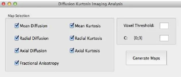
As soon as the DKI plugin is selected, the method filterImage is activated

and summons the user interface window shown in figure 3.3. This interface offers

36

the value for 𝐶, within the range mentioned in equation (31). It is also possible to set a threshold for voxel values under which no computation is conducted and

all 𝐷_𝑖′𝑠 and 𝐾_𝑖′𝑠 are set to zero.

Figure 3.3: The DKI plugin graphical user interface (GUI).

On clicking the “Generate Maps” button, the user initiates the DKI compu-tation by triggering the plugin’s main function, GenerateMaps.

This function starts by reading the input values appointed by the user on

the graphical interface for variables 𝐶 and MinPixValue, where the latter stands

for the threshold for voxel computation. The value for 𝐶 is checked so as to assure it falls into the allowed range. Otherwise, the 𝐶 is set to its default value of 3

following an alert box with the message “Invalid 𝐶 value. 𝐶 was set to its default value of 3.”.

37

Afterwards, the plugin reads the array (NSArray) containing the DWI’s of

the selected study and gets the number of slices (PIXCOUNT), the size of the

images (SIZE) and the number of gradient directions (ndir).

At this point, the b-values and gradient directions are read from the image’s

metadata and their values are stored into two arrays using the functions infigure

3.4

Figure 3.4:Code for acquiring the gradient directions and b-values from the metadata of the DWI set.

where img is the current image being read and “@"DiffusionGradientOrienta-tion”” and “@"Diffusionb-value"” are the metadata tags for the gradient direc-tions and b-values respectively.

Because the tags for these parameters may not be the same for different ven-dors, in order for the plugin to work regardless on the MRI vendor, a more ver-satile function must be developed. The implementation of such function is sug-gested in the future work section.

The b-values are subsequently compared and stored is ascending order as B0, B1 and B2.

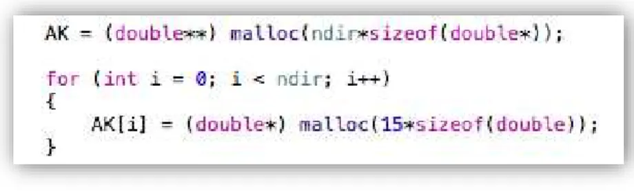
Having gathered all the gradient directions, memory must be allocated for two 2D arrays which will be populated according to equations (35, 36, 39 and 40) to represent both 𝐴_𝐷 and 𝐴_𝐾 matrices. To allocate the exact necessary memory, the dimensions of the matrices must be known. In this case the dimensions for

𝐴𝐷 and 𝐴𝐾 are [6 x ndir] and [15 x ndir] respectively.