Auction Econometrics by Least Squares
Leonardo Rezende
∗Dept. of Economics, University of Illinois
1206 S Sixth St., Champaign, IL 61820, U.S.A.
[email protected]
June 15, 2004
Abstract
This paper proposes a method to structurally estimate an auction model using a variation of OLS, under commonly held assumptions in both auction theory and econometrics. In spite of its computational simplicity, the method applies to a wide variety of environments, in-cluding interdependent values in general, and certain forms of endoge-nous participation and bidder asymmetry. Furthermore, it can be used for hypotheses testing about the shape of the valuation distribution, valuation interdependence, or existence of bidder asymmetry.
1
Introduction
The advent of online auction houses such as eBay has made accessible a vast amount of data to economists. Because such websites provide information on a large number of individual transactions among a wide variety of buyers and sellers on a huge set of products, they allow for a much more detailed investigation about consumers preferences than it was previously possible.
∗Based on chapters 4 and 5 of my Ph.D. dissertation at Stanford University. Still
Studies that seek to understand how covariates affect demand in auction markets often run regressions like that:
p=Xβ+ǫ, (1)
where p is the transaction price (or its log). To provide a specific example, several studies investigated the importance attributed by consumers to the reputation of sellers in eBay using specifications of this sort (Houser and Wooders, 2000; Lucking-Reiley, Bryan, Prasad, and Reeves, 2000; McDonald and Slawson, 2002; Melnik and Alm, 2002).
The problem with analyses that rely on such specification is not in the right-hand side of regression — covariates may indeed impact consumer pref-erences in a linear fashion — but rather in the left-hand side. A superior starting point for an empirical analysis would be a specification like
Vi =Xβ+ǫi, (2)
whereViis consumeri’s valuation, or willingness to pay, for the product being
auctioned. Unlike price, a valuation is a demand concept, that reflects the consumer’s preferences in isolation of effects through supply or the market institutions. A bidder will never elect to pay his or her own valuation for the product — doing so would guarantee that that the bidder would not gain anything from participating in an auction. Because of that, we know prices and valuations are not supposed to be the same. Therefore, whenever the objective is to measure consumers’ preferences, a regression like equation 1 would suffer from misspecification bias.
Auction theory tells us however that, given a precisely defined auction en-vironment, one can obtain a mapping between valuations and observed bid-ding behavior and from that mapping develop estimation strategies. Laffont and Vuong (1996) have shown that, depending on the auction protocol, the valuation distribution is just identified from bidding data. Several methods have been developed to estimate valuations from auction data: for exam-ple, Laffont, Ossard, and Vuong (1995) have proposed a simulated nonlinear least squares methodology; Donald and Paarsch (1993) have introduced a piecewise pseudo-maximum likelihood estimator; and Guerre, Perrigne, and Vuong (2000) have shown how to obtain fully non-parametric estimates of the valuation distribution.
played and they are computationally complex. This state of affairs may lead to the perception that applied work with auction data informed by auction theory would necessarily lead to overly complex and specific empirical proce-dures, and that, for researchers unwilling to adopt them, the only alternative is to rely on misspecified regressions like equation 1.
This is not true. The objective of this paper is to show that, starting from a specification like equation 2, one can obtain an estimation method that is at once structural, justified by auction theory, computationally simple and robust to several types of misspecifications of the auction game being played. In fact the method proposed involves a running an ordinary least squares regression of observed transaction prices in the covariates of interest and an additional regressor involving the number of bidders in each auction. So com-putationally the method is as straightforward as running an OLS regression, involving variables that are readily observable in an auction dataset. There is no need for example to use information on losing bids, that is often not observable or not reliable from theoretical and practical grounds.1
And yet, the method is fully theoretically justified. It also remains valid in a wide variety of auction rules and assumptions about how valuations are related, including the independent private values case and the common values case. It also robust to several versions of endogenous or hidden entry, and can also accommodate some forms of bidder heterogeneity.
A second product of the methodology is that it provides not only infor-mation about the impact of covariates, but also delivers in a computationally cheap way a significant amount of information about the shape of the valua-tion distribuvalua-tion within each aucvalua-tion. In particular, it provides informavalua-tion about the valuation of consumers at the top end of the demand curve. This allows for estimates of consumer surplus that do not rely solely on arbitrary functional assumptions about the shape of the demand curve near the ver-tical axis. The discussion on how to explore the method to obtain such information is done in section 6.
This work is related to several strands in the empirical literature on
auc-1In English Auctions for instance Bikhchandani, Haile, and Riley (2002) have shown
tions. The regression proposed, involving winning bids in the left hand side and the number of bidders in the right hand side, is similar to regressions ran both in the reduced form literature (Gilley and Karels, 1981, e.g.) or as an initial step in the structural literature (Paarsch, 1991, e.g.). The main difference is that, unlike in those papers, here this regression is fully justified in theoretical grounds.2
The method here will exploit two import properties of auctions: the Revenue Equivalence Theorem and the invariance of the set of equilibria to affine transformations on valuations (see Proposition 2 below). Both ideas have been used elsewhere, but not simultaneously: Laffont, Ossard, and Vuong (1995) use the Revenue Equivalence Theorem to justify their sim-ulated NLLS methodology; versions of the invariance property are used in Bajari and Horta¸csu (2003), Deltas and Chakraborty (2001) and Krasnokut-skaya (2002). However, these papers do not combine both ideas; as a result, their methodologies are either computationally demanding, applicable to a limited class of auctions, or both.
The paper is organized as follows: Section 2 introduces the method in the classic independent private values framework. Sections 3 to 5 discuss the robustness of the method in more general contexts: Interdependent values are discussed in section 3; bidder heterogeneity is discussed in section 4; and various types of endogenous or hidden participation are discussed in section 5. The possibility of exploiting the information obtained from the method for inference about valuations distributions is discussed in section 6, and illustrated by an practical application on a sample of Palm Pilot eBay auctions in section 7. Section 8 concludes.
2
The Basic Method
With minor modifications, the method proposed in this paper applies to a variety of symmetric auction models, including auctions with interdependent values and endogenous entry. For the sake of expositional clarity, it is conve-nient to present the method first in the context of the benchmark model in auction theory: the independent private values model. This is done in this section. Sections 3–5 discuss the necessary changes to accommodate a richer
2Also, in most cases these regressions include the number of bidders in a linear or
Proposi-set of assumptions.
Let Vil be the valuation of the i-th bidder in the l-th auction. Let µl
be the mean and σl the standard deviation of valuations in auction l. As
the subscript suggests, they may vary across auctions. We will assume that variation across auctions only affects the location and scale of valuations, not other aspects of the valuation distribution:
Assumption 1 Vil =µl+σlǫil, where the ǫil are i.i.d. with distribution F.
The normalized valuation,ǫil = (Vil−µl)/σl, has a common distribution
F that does not vary across auctions or bidders. For the moment we also impose independence, both across auctions and bidders.
Independence across different auctions is an assumption made here for mere convenience. Relaxing it in what follows would have the same effect of having non-spherical disturbances in a linear regression model: it would affect efficiency, but not unbiasedness of the estimators.3
Independence across bidder valuations within an auction is one of the central characteristics of the benchmark model in auction theory, the inde-pendent private values auction model. Imposing indeinde-pendent private values simplifies the analysis somewhat, but is not necessary: see Section 3 for an extension to the much more general interdependent values case.
The first object of interest of the researcher is to evaluate the effect of covariates on µl and σl. Let Xl be the vector of covariates that affect the
expected valuation µl and Zl the vector of covariates that affect σl. We
assume that [Xl, Zl] are either deterministic or otherwise publicly known by
all bidders before auction l starts. Linearity is imposed:
Assumption 2 µl=Xlβ. σl =Zlα.
We intend to obtain estimates of β and α from a sample of auctions of which we know the covariates [Xl, Zl], the number of bidders nl and the
winning pricepl. The method will exploit the central result in auction theory,
the Expected Revenue Equivalence Theorem. Besides independent private values, we impose
Assumption 3 The number of bidders,nl, is exogenous and common
knowl-edge. Bidders are risk-neutral, and maximize their profits at each auction in isolation.
3In any case, spherical disturbances in equation 2 is not enough to guarantee efficiency
Here exogeneity is meant both in the game theoretic sense —nl is taken
as given, and is not determined by each bidder decision-making process — and in the econometric sense — ǫil and nl are independent. The number of
bidders is also assumed to be publicly known before bidding. Both hypotheses can be relaxed somewhat: See Section 5 for details.
One remarkable advantage of the Independent Private Values framework is that it allows the method to be unaffected by the details of the auction pro-cess: The same method applies to any standard auction rule. More precisely, we require that
Assumption 4 The auction rules are such that the good is always assigned
to the bidder with the highest value, and the lowest valuation bidder expects to pay nothing.
This is a condition satisfied by the English auction, the sealed-bid auction, the second-price auction, and also by the all-pay auction.4
Although this is an admittedly long list of assumptions, they are quite conventional. In fact, assumptions 3, 4 and independence and identical distri-bution of valuations within an auction are the conditions for an independent private values model, the classical auction-theoretic framework introduced by Vickrey (1961). Assumptions 1 and 2 are typical in Econometrics; if for example F is standard normal and Zl included just the intercept we would
obtain the classical regression model for Vil (except for the fact that Vil is
not observed). A richer Zl allows for heteroskedasticity.
The method explores the central result in auction theory, the Expected Revenue Equivalence Theorem (Vickrey, 1961; Myerson, 1981):5
Theorem 1 (Expected Revenue Equivalence) Under assumptions 1, 3
and 4, the expected payment for the good in auction l is E[V(2:nl)l].
Here the expectation is taken with respect to all information that is pub-licly available at the time of the auction; therefore the Expected Revenue Equivalence Theorem establishes that E[pl|Xl, Zl, nl] =E[V(2:nl)|Xl, Zl, nl].
4In the case of an all-pay auction, p
l should be interpreted as the sum of the prices
payed by all bidders, rather than the amount payed by the winner.
5In what follows the notationx
(k:n) represents thekth-highest order statistic from an
2.1
Estimation
Suppose a dataset of auctions is available with information about the final selling price pl, the number of bidders nl and covariates [Xl, Zl]. Then under
the assumptions made we can write
E[pl|Xl, Zl, nl] = E[V(2:nl)|Xl, Zl, nl]
= E[µl+σlǫ(2:nl)|Xl, Zl, nl]
= µl+σlE[ǫ(2:nl)],
where the first equality is due to the Expected Revenue Equivalence Theorem, the second is due to the specification of the location and scale parameters, and the third by the definition of conditional expectation. Defining a(n) =
E[ǫ(2:n)],
E[pl|Xl, Zl, nl] = Xlβ+Zlαa(nl). (3)
Note that the conditional expectation of the winning bid is linear in β
andα. This means that OLS is an unbiased, consistent estimation method to estimate these coefficients. This observation gives rise to two straightforward procedures to estimate β and α: If the researcher is willing to impose a particular choice for the shape of the distribution of values, the following method is suggested:
Method 1 Using the assumed shape of the normalized value distribution,
compute a(nl) for all values of nl in the sample. Construct the set of
regressors [Xl, a(nl)Zl], and run OLS of the observed winning bids on
these regressors.
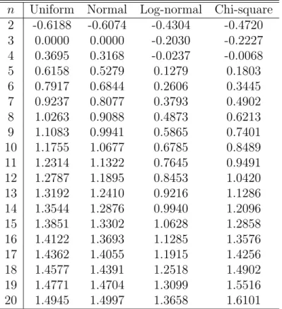
The first step requires the computation ofa(n) =E[ǫ(2:n)] for the specified
distribution of ǫ. These calculations are shown for some normalized distri-butions in Table 1 below. After this calculation is done, unbiased estimates of the parameters can be obtained by OLS.
It is important to notice that method 1 is not the same as introducing
nl as an additional regressor, as is often done in the literature, but rather
it entails introducing a(nl), a nonlinear function of nl. In fact, ignoring the
n Uniform Normal Log-normal Chi-square
2 -0.6188 -0.6074 -0.4304 -0.4720
3 0.0000 0.0000 -0.2030 -0.2227
4 0.3695 0.3168 -0.0237 -0.0068
5 0.6158 0.5279 0.1279 0.1803
6 0.7917 0.6844 0.2606 0.3445
7 0.9237 0.8077 0.3793 0.4902
8 1.0263 0.9088 0.4873 0.6213
9 1.1083 0.9941 0.5865 0.7401
10 1.1755 1.0677 0.6785 0.8489
11 1.2314 1.1322 0.7645 0.9491
12 1.2787 1.1895 0.8453 1.0420
13 1.3192 1.2410 0.9216 1.1286
14 1.3544 1.2876 0.9940 1.2096
15 1.3851 1.3302 1.0628 1.2858
16 1.4122 1.3693 1.1285 1.3576
17 1.4362 1.4055 1.1915 1.4256
18 1.4577 1.4391 1.2518 1.4902
19 1.4771 1.4704 1.3099 1.5516
20 1.4945 1.4997 1.3658 1.6101
Proposition 1 There is no non-degenerate distribution F such that a(n) is affine in n.
Because the proof of this proposition depends on tools that will be devel-oped in section 6, it will be deferred to section 6.3.
Unbiased estimators for α and β do depend on introducing an appro-priately chosen nonlinear function of the number of bidders as an additional regressor, and the appropriate function depends on the shape of the valuation distribution. Often, however, one may be unwilling to commit to a specific assumption about the valuation distribution. In that case, one can still ob-tain unbiased estimates for α and β using instead the following method:
Method 2 Run OLS of the observed winning bids on Xl and interactions
of Zl and dummies for eachnl in the sample.
Method 2 has the advantage of allowing the researcher to be agnostic about the shape of the valuations distribution. It requires constructing dum-mies dkl for the event nl = k for every k in the support of nl, and then
running an OLS regression of pl onXl and interactions ofZl and dkl.
An interesting feature of method 2 is that the pattern of the estimated dummy coefficients contains information about the shape of F — in fact, it will be shown in section 6 that the sequence {a(n)}∞
n=2 identifies F. This
gives rise to the possibility of using the dummy estimates for inference about the shape of F. Section 6 discusses this possibility in detail.
3
Interdependent Values
For expositional clarity, the presentation of the method in the last section was done under the assumption of independent private values. However, this assumption is not at all necessary. This section shows that the method works essentially unchanged for virtually any other information structure and most auction rules (including all commonly observed auction rules).
To describe the necessary conditions on the auction rules, letbi to be
bid-der i’s “bid” in a given auction (The quotation marks here are used because
bi does not necessarily need to be a bid per se; it is simply a way to describe
i’s action.) In most auctions, bi is taken to be a number (but not necessarily
a payment promise); all that will be needed here is that bi be a member of
Wi(b) be i’s (expected) probability of winning the item given that bidders in
the auction played b, and let Pi(b) be the expected payment given b.
Let vi be i’s valuation (not necessarily private or independent), let v =
(v1, . . . , vn), and let µand σ >0 be constants. Then we have the following:
Proposition 2 Suppose an auction rule is such that (i) Wi(µ+σb) =Wi(b)
and (ii)Pi(µ+σb) = µ+σPi(b), for alli. Then, ifβ = (β1, . . . , βn)is a Nash
equilibrium of an auction when bidders have valuations v, then µ+σβ is a Nash equilibrium of the auction when valuations areµ+σv. As a consequence, if the expected selling price in the first auction is p¯, then the expected price in the second auction will be µ+σp¯.
Proof: Forβ to be a Nash equilibrium underv, it must be that it prescribes
i to bid
argmax
bi
E[viWi(b)−Pi(b)],
where this expectation is taken to be conditional on all information available to i (including the contingency of winning), andb−i followsβ−i.
In the game with valuationsµ+σv, by followingµ+σβ bidderiachieves
E[(µ+σvi)Wi(µ+σb)−Pi(µ+σb)] = E[µ+σviWi(b)−(µ+σPi(b))]
= σE[viWi(b)−Pi(b)].
Clearly, any bi that solves the first problem solves the second as well.
As for the expected selling price, this is a consequence of this result combined with the affinity of Pi.
Notice that the two conditions onWi and Pi are satisfied by all common,
and many uncommon, auction rules. For example, the condition on Wi
is satisfied by any rule that assigns a winner based on a ordering of the bids. This includes all standard auctions, that assign the good to the highest bidder, and many non-standard auctions, that for example assing the good to the k-th highest bidder.6
6It may may be worthwhile to point out that this assumption implictly imposes some
restrictions on reserve prices. ForW to have the desired property, either the reserve price
rmust be trivial (in the sense that the probability ofvi andµ+σvi be belowris zero) or
The condition onPi is also very easily met; any auction where payments
depend linearly on a bidder’s own bid (as in a first price auction or the all-pay auction) or somebody else’s bid (as in the Vickrey or English auctions) will satisfy it.
For our purposes proposition 2 is very important because it implies that, in any auction equilibrium, we can write something very similar to equation 3, namely,
E[pl|Xl, Zl, nl] = Xlβ+Zlαa˜(nl), (4)
where ˜a(nl) = E[˜pl|nl] and ˜pl is the selling price from an auction where
bidders have normalized valuations.
So for estimation purposes the only impact of relaxing the IPV assump-tion is that the first step in method 1 involves calculating a different ˜a func-tion, a function that depends not only on the distribution of the normalized values, but also on their statistical dependency, their relation with the bid-ders’ information, andthe specific auction rule (recall that without IPV rev-enue equivalence no longer holds). Appendix A illustrates these calculations for several affiliated values models.
Such calculations might be quite hard in particular instances, but for-tunately for researchers interested in only estimating β and α they are not necessary. From equation 4 we learn that method 2 would work here in exactly the same manner without requiring the researcher to commit to a specific informational structure or auction rule.7
4
Asymmetry
Another important assumption imposed in section 2 is that bidders are sym-metric, in the sense that within auction their ex-ante value distribution is the same. On the other hand, as the discussion in section 3 suggests, the driving property of auction models that validates the method is Proposition 2, and it does not depend on symmetry. This suggest that the method can also accomodate asymmetric auctions. This section discusses this possibility.
For concreteness, suppose we consider an auction where bidders come from two different categories (say, “A” and “B”). Bidders from different
cat-7That of course assumes that no other changes occur in the sample. If, for example,
egories obtain their values from different distributions, and this distinction is publicly known (that is what makes this model fundamentally different from a symmetric one). Let nA
l and nBl be the number of bidders from categories
A and B that participate in auction l. Then, in light of Proposition 2, we have
E[pl|Xl, Zl, nAl , nBL] = Xlβ+Zlαa(nAl , nBl ), (5)
wherea(nA
l , nBl ) is the expected price of a normalized auction withnAl bidders
of category A and nB
l of category B.
The same regression strategies would still work, but now the nonlinear function ˜a is somewhat more complex. Not only it is now a function of two rather than one index, but calculating it would require finding an equilibrium of an asymmetric auction. This can be hard; for example, in first-price auctions that would involve solving a system of ordinary differential equations (Lebrun, 1996; Bajari, 1999).
Another difficulty with the asymmetric setting is in how to exactly inter-pret µl and σl (or, equivalently, on how to normalize valuations). It would
probably be desirable to have a definition based on means and standard de-viations from each category’s valuation distributions; while it is clear that they are related with µl and σl, the relationship is far from transparent, and
is dependent on the specific nature of the asymmetry.
In any case, here again method 2 is applicable, provided that we allow dummies for bothnA
l andnBl , and does not require specifying the exact nature
of the asymmetry, let alone computing equilibria of asymmetric auctions. The estimated β and α would not provide information about the exact nature of the asymmetry (e.g., they would not tell which group tends to have higher values), but they would provide information on how covariates affect valuations in a way that is robust to asymmetry.
Furthermore, the values of the dummy coefficients can be used to test whether symmetry is present (or more precisely, whether it significantly im-pacts selling prices). To test where valuation distributions are across cate-gories Aand B, a researcher can run a regression of equation 5 by method 2 and then perform a linear hypothesis test, where the null hypothesis of sym-metry corresponds to the restriction a(nA, nB) =a(nA+nB) for all values of
5
Endogenous or Hidden Participation
So far the analysis has relied on the hypothesis that the number of bidders in each auction is determined exogenously and is common knowledge among bidders. This is a conventional assumption in the auction theory literature, but may not necessarily hold in practice. Because the number of bidders play such an important role in the estimation strategy, it is appropriate to discuss how alternative hypotheses about bidder entry would affect the estimation method.
This section discusses three possible alternative hypotheses: endogenous entry prior to learning about values, endogenous entry after learning about values, and exogenous hidden entry.
5.1
Why the Timing of the Entry Decision is
Impor-tant
A natural way to formalize the entry decision process is to assume that prior to participating in the market bidders face an entry cost. This cost may be related to the process of searching for the auction and evaluating the item being sold, or can be related to the effort to submit a bid. This distinction is important, because in the first case bidders must decide to enter and incur the cost before they know the value they attach to the item (ex-ante endogenous entry), while in the second case they do so after they know their value (interim endogenous entry).
Statistically, the distinction can be described as following: let N be the original number of potential bidders in a given auction, that is typically not observed by the econometrician directly. Let as before n ≤ N be the number of bidders that participate. Let λi be the probability that bidder i
participates. The crucial distinction between ex ante endogenous entry and interim endogenous entry is that they predict different correlation paterns betweenλiandǫi. In ex-ante endogenous entry models,λiis independent ofǫi
(and typically assumed to be the same across bidders); in interim endogenous entry models, λi = Pr(ǫi > c), where c is a threshold that depends on the
5.2
Ex Ante Endogenous Entry
The case of ex-ante endogenous entry has been studied by McAfee and McMillan (1987b) and Levin and Smith (1994), among others. McAfee and McMillan (1987b) studied asymmetric equilibria where a deterministic num-ber of bidders enter; Levin and Smith (1994) focused on the symmetric, mixed strategy equilibrium of the same game. In either case, as long as the number of bidders that eventually enter is common knowledge when bidding is decided, bidding behavior is not affected.
As long as participation is large enough (n ≥2), information aboutN is not necessary to estimate β and α: If the parameterization of the value in Assumption 1 is still valid, the methods work unchanged. The number of bid-dersn is endogenous in the game-theoretic sense, but not on the econometric sense. Variation in n can be explained by (unobserved) variation in entry costs or by the realizations of a mixed strategy equilibrium. An economet-ric endogeneity problem would arise only if ǫ is correlated with information observable by bidders prior to entry that would affect their entry decision.
Auctions with little or no participation (n ≤ 1) obviously cannot be included in the regression, since for them the expected price does not obey equation 3. Censoring out such auctions might however bring up a sample selection problem.
The ex-ante endogenous entry model provides a justification for not wor-rying about sample selection bias. As long as the values within an auction (and therefore the residuals) are independent from the variables that deter-mine entry, then no sample selection bias exists. In this theory low parti-pation would be explained through either a low number of initial potential bidders (N) or high participation costs, and not through an unobserved value component.8
5.3
Interim Endogenous Entry
Another possibility is that the entry decision happens after bidders learn about their value (Samuelson, 1985). This assumption is appropriate if the entry cost is related to the bidding process itself, rather than finding the auction or evaluating the value of the product.
8Here one would need to assume that participation costs are independent of the
Consider a situation where there are N potential bidders with indepen-dent private values, but in order to bid they must pay an entry cost. A bidder would enter if the expected payoff in the auction is enough to cover the entry cost. Since the expected payoff is increasing in the bidder’s valua-tion, there will be a cutoff such that bidders with values above it enter and those below it stay out. In this case, the probability of i entering would be
λi = Pr(ǫi > c), a function of ǫi. (Notice that this would also happen in the
presence of a reserve price.)
So the entry process distorts the valuation distribution of entrants — it truncates it below. However, the expected transaction price is still a second order statistic. So the methods proposed here would still work, provided that the researcher used the number of potential bidders N rather than the number of actual bidders.
Unfortunately in practice the number of potential bidders is seldom ob-served by the econometrician. In these circumstances substituting the actual number of bidders would lead to specification bias. The next two sections discuss two ways to account for lack of direct information about N in the estimation.
5.3.1 Nonlinear Error in Variables
One way to proceed, bar direct knowledge of N, would be to assume the re-searcher has access to a setW of proxies for it. Assuming a linear relationship between N and W, we could perhaps write
N =W γ+u, (6)
where u is an error term (possibly assumed to be independent of {ǫi}). In
that case, however, the initial regression would read
p=Xβ+Zαa(W γ+u) +η,
something that cannot be estimated in a straighforward fashion given the non-linearity ofa(·). This is a nonlinear error-in-variables model. Because of the nonlinearity aroundN, such a model cannot be estimated by instrumental variables.9
9Y. Amemiya (1985) has argued that, unless the variance of u goes to 0, IV is not
Some estimation procedures have been suggested that rely on validation data, an auxiliary sample that contains information about the relationship between N and W (Lee and Sepanski, 1995). Similarly, Newey (2001) pro-poses a simulated method of moments estimators that integrates out the measurement error u; but his model requires observability of a direct proxy for N. More specifically, he assumes the researcher observes both W and ˜N, that are related to the true N according to equation 6 and
˜
N =N +ζ,
where ζ is an error, with E[ζ|W, u, η] = 0. In his method, observability of ˜N
not only helps estimating γ (since E[ ˜N|W] = W γ), but it is also necessary for the identification of the main regression: “Intuitively, two functions need to be identified — the regression function and the density of the measurement error — so that two equations are needed for identification” (Newey, 2001, p. 617).
This suggests that one could avoid needing validation data by imposing a specific distribution for the measurement error. Hong and Tamer (2003) show that this is in fact true; ifuis double exponential, than one can accomo-date error-in-variables in a standard method of moments procedure without validation data by adding a correction term that depends on the curvature of the nonlinear regression function and the variance of the measurement error. Unfortunately, assuming that the measurement error is double exponential may not be reasonable in this application, since N is a discrete variable. It does suggest however that is may be possible to estimate regressions 3 and 6 without further data, under additional assumptions about the distribution of u.
5.3.2 Systematic Relationship between n and N
An alternative that avoids the non-linear error in variables problem is to assume that the entry process is such that, conditional on observable intru-mentes W, there is a systematic relationship between the observed number of bidders n and the potential number of bidders N we are interested in:
n =φ(W, N). (7)
relationship and write10
N =ψ(W, n),
so that
p=Xβ+Zαa(ψ(W, n)) +η=Xβ+Zα˜a(W, n) +η. (8)
Estimation would be straightforward: all that is needed is to allow ˜a do depend not only on n, but onW as well.
While this idea provides an easy way out of the problem of not observing
N, unfortunately it is not fully justifiable in theoretical grounds. Natural theories of entry that justify focusing on N in the first place would predict that the relationship betweennandN will not be deterministic; for example, the model discussed in section 5.3 would predict thatn is a binomial random variable from a sample of size N. It is not clear whether it is possible to find a reasonable model of endogenous entry that would simultaneously justify using N in equation 3 and yet have N and n be deterministically related as in equation 7.
5.4
Exogenous Hidden Entry
Another aspect of entry that is important in the analysis is whether bid-ders know the number of competitors before bidding. McAfee and McMillan (1987a) have studied how lack of knowledge about the number of bidders affects the properties of an auction.11
The way hidden entry affects the method will depend on the specific auction rule. In an English or a Vickrey auction bidders do not use infor-mation about the number of competitors in their strategies; therefore lack of knowledge about it does not have any effect.
In a first price auction, equilibrium bidding strategies do depend on the number of bidders. So if required to bid without knowing n, a bidder will have to follow a strategy that maximizes the expected payoff over the range of possible values forn. That would lead to a different equilibrium bid strategy, and therefore a different expected price, depending on whether n is hidden or not.
10This “trick” is originally due to Olley and Pakes (1996), and has been used otherwise
in the empirical auction literature by Campo, Perrigne, and Vuong (2001) and Haile, Hong, and Shum (2003).
McAfee and McMillan (1987a) show that a version of the Expected Rev-enue Equivalence Theorem is still valid: the expected price of a first-price auction with hidden n is the same as the English or Vickrey auction, and therefore also of a first price auction with knownn. However, this is not suf-ficient for the applicability of the method. Revenue equivalence holds only ex-ante, for the unconditional expected price. For the method to work un-changed we would need instead equivalence of the expected price conditional on n. If the econometrician uses the methods described here with informa-tion about n that was not available to the bidders in a first price auction, the regression would be misspecified, since compared with predicted behav-ior bidding would be too aggressive in auctions with few bidders and not aggressive enough in auctions with many bidders.
6
Identifying Distributions from Least Squares
Coefficients
Besides providing unbiased estimates for parameters that determine the loca-tion and scale of the value distribuloca-tions, the method proposed in this paper also provide indirect information about the underlying shape of the valuation distribution through the estimated pattern of a(n)’s.
This section discusses ways to explore this information. It establishes that this information is enough to fully identify the valuation distribution: in other words, in principle it is possible to obtain a nonparametric estimator of the valuation distribution from the estimated coefficients of an ordinary least squares regression!
It also provides a straightforward test for specific distributional assump-tions. The methodology is illustrated in the next section with an application to a dataset of Palm III PDA auctions from eBay.
6.1
Full Identification of
F
from
{
a
(
n
)}
A perhaps surprising fact is that a distribution can be fully identified from knowledge of its a(n)’s. This has been shown in several versions in the Statistics literature (Hoeffding, 1953; Chan, 1967; Pollak, 1973). Here a constructive proof is provided, that directly shows how to compute F from
{a(n)}∞
Theorem 2 Suppose that F has a finite expectation. Then there is a one-to-one mapping between F and the sequence {a(n)}∞
n=2.
The overall strategy of the proof follows Pollak (1973): the construction of F froma(n) will be made in two steps, that we state as lemmas.
Lemma 1 (recurrence relation) Letω(k:n)=E[ǫ(k:n)], for alln = 2,3, . . .
and all k = 2,3, . . . , n. Then the following recurrence relation holds:
ω(k:n−1) =
n−k
n ω(k:n)+ k
nω(k+1:n).
Proof: See appendix B.
Corollary 1 Knowledge of a(n) = E[ǫ(2:n)] for every n = 2,3, . . . is
suffi-cient to know all ω(k:n) =E[ǫ(k:n)], for all n= 2,3, . . .and all k = 2,3, . . . , n.
Proof: See appendix B.
Observe that the recurrence relation is valid for any random variable (with finite expectation). If the mean (=ω(1:1)) of it is known, then one can
further compute ω(1:n) using the recurrence formula. However, this will not
be needed in what follows.
Another remarkable fact is that the same recurrence relation is valid for the expectation of any measurable function g of the order statistics:
E[g(ǫ(k+1:n))] = nkE[g(ǫ(k:n−1))]−
n−k
k E[g(ǫ(k:n))]. So the same lemma applies
to other moments, such as the variance of the order statistics.12
Lemma 2 Let{kn}be a sequence of integers such that1−kn/n→α ∈[0,1].
Then ǫ(kn,n)→F
−1
(α) in probability.
Proof of Theorem 2: To obtain the quantile F−1
(α) for any α ∈ [0,1], select a sequence{kn}such thatkn≥2 andkn/n→1−α. Use the recurrence
formula to compute ω(kn:n) from the a(n)’s, and then take the limit. The
converse is immediate.
12Another application of the recurrence relation in Economics can be found in Athey
In principle Theorem 2 provides a way to obtain a non-parametric esti-mate of the distribution of F by ordinary least squares. From method 2 we obtain estimators ˆa(n) that are unbiased and consistent for a(n). Since the recurrence formula is linear, the corresponding ˆω(k:N) are also unbiased and
consistent (for a fixedN, as the number of auctions goes to infinity). Finally, for large N, from lemma 2 the expectation of these estimators converges to the quantiles of the original distribution.
However, it should be kept in mind that the linear combinations that arise from the recurrence formula have large coefficients of opposing signs. So the variance of ˆω(k:n) can be very large even if the ˆa(n) are estimated precisely.
So the method of the last paragraph is likely to perform very poorly even in a very large dataset.
Using the recurrence formula, the following closed form expression for
ω(k:n) can be obtained:
ω(k:n) =
n!
(n−k)!(k−1)!
k−2 X
j=0
(−1)k−j−2 (k−2)!
j!(k−2−j)!
a(n−j) (n−j)(n−j−1).
Soω(k:n) is a linear combination of the k−1 previous a(n)’s, with
coeffi-cients that alternate signs. As k and n grow, not only the number of terms in the sum grow, but also do the coefficients. This means that the estimator for ω(k:n) is likely to have a variance too large to be of practical use.
To see that, consider the case where there are no covariates for the the mean and variance of the valuations (µl = 0 and σl = 1). In this case the
estimators for ˆa(n) are means of different auction subsamples, and are there-fore independent. In this case, the variance of ˆω(k:n) is simply Var(ˆω(k:n)) = Pk−2
j=0c(j, k, n)2Var(ˆa(n−j)), wherec(j, k, n) =n!/((n−k)!(k−1)!)(k−2)!/(j!(k−2−j)!(n−
Suppose we are interested in estimating the median of the valuation dis-tribution, and for that we use ˆω(n/2:n) for some large choice of n. Take the
first coefficient c(0, k, n). For k =n/2 we find
c(0, k, n) = n!
(n−k)!(k−1)!n(n−1) =
(n−2)! (n−k)!(k−1)!
≃ n!
((n/2)!)2 n−→→∞ ∞.
reason, one should not expect to obtain accurate estimates of quantiles of F
using this direct method.
However, that theoretical result indicates that there is a significant amount of information in {a(n)}; in particular, about aspects of the shape of the up-per tail that are of interest to study revenue and surplus issues. The next section discusses a practical way to explore this information.
6.2
Hypothesis Testing about Distributions
Perhaps the easiest and most useful way to use the information contained on the ˆa(n) estimators is to test for the hypothesis of a specific distribution F. Under the null hypothesis that a givenF is the normalized valuation dis-tribution, method 1 would be appropriate. Under the alternative hypothesis, method 2 would be. But the regression by method 1 is a restricted version of the regression in method 2, where the a(n) terms are required to follow the shape specified by F. So one can simply test the hypothesis by running both methods and applying an F-test on the R2 difference. This procedure
is illustrated in section 7. In an application to data on Palm III auctions, this method succeeds in indicating that the distribution of bidder valuations is log-normal — a distribution that is often thought to be appropriate for valuations in auctions.13
Of course, this idea is not restricted to the IPV class of distributions; any distribution of values to which one can compute equilibrium bids and therefore the corresponding a function can be tested in the same way. Sec-tion 7.1 provides an illustraSec-tion by testing and rejecting several common values models for Palm Pilot eBay auctions.
13IfF is known up to a family of distributions indexed by a set of parametersθ, a similar
idea can be used in a two step procedure to estimate θ.
Assume that ǫil is drawn from a distribution F ∈ {Fθ}θ, where {Fθ}θ is a family
parameterized by θ. We are interested in findingθ such thatF =Fθ. Then, for everyn
observed in the sample, we can use the moment condition
a(n) = n! (n−2)!
Z
xF(n−2)
θ (1−Fθ)dFθ
6.3
Non-linearity of
a
(
n
)
An important observation to be made from Table 1 is thata(n) is not linear. In fact, a(n) is never linear, as proposition 1 establishes:
Proof of proposition 1: Suppose there was such distribution. Leta(n) =
ω(2:n) =c+bn for some constants c and b. We must necessarily have b ≥0.
If b = 0, by the mapping from Theorem 2 it is easy to verify that the distribution is degenerate. So we must have b >0.
Now, successively apply the recursion formula to the case where k = 1. We obtain
ω(1:n) =
n
n−1ω(1:n−1) −
c+nb n−1
= n
n−1
n−1
n−2ω(1:n−2)−
c+ (n−1)b n−2
− c+nb
n−1
= nω(1:1)−
n
n(n−1)(c+nb)−
n
(n−1)(n−2)(c+ (n−1)b) +· · ·
= n
ω(1:1)−c
1
n(n−1) +
1
(n−1)(n−2)+· · ·
−b
1
n−1+ 1
n−2 +· · ·
→ −∞,
as n→ ∞, since the sum that multiplies b diverges (while the one that mul-tiplies cdoes not). This contradicts the fact that ω(1:n) should be increasing
in n.
Therefore, running a reduced-form regression of the winning bid with the number of bidders being treated as a linear regressor will always lead to misspecification bias, even when it is correct to assume that the number of bidders n in each auction is exogenous.
7
An Application to the Palm Pilot Market
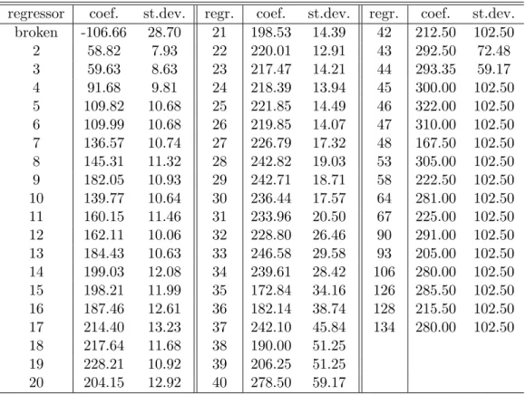
We have introduced as covariate for the mean a dummy for the object being described as broken, and no covariate for the variance. Unfortunately there is no data on the number of bidders per auction in this sample, and the number of bids have been used in its place. That potentially overestimates the number of bidders. Although, under the proxy bidding rules used in eBay, bidders do not have an incentive to bid more than once, if valuations are independent.
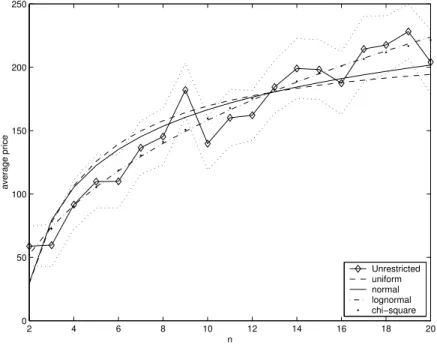
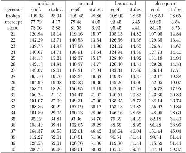
Estimated coefficients for all regressions are reported in Tables 5 and 6 at the end of the paper. Figure 1 presents graphically the estimated a(n)’s, obtained with the method 2 and the corresponding estimated expected trans-action prices under the assumption that ǫ has uniform, normal, log-normal or chi-square distribution.14
2 4 6 8 10 12 14 16 18 20 0
50 100 150 200 250
n
average price
Unrestricted uniform normal lognormal chi−square
Figure 1: Estimated a(n)’s, Palm Pilot III regression.
The more concave lines are the a(n)’s of the uniform and normal distri-bution. The least concave lines, that seem to fit the data better, correspond
14Because the number of auctions with many bids is small (cf. Table 7 at end of the
to the distributions with a thicker upper tail, namely the log-normal and chi-square.
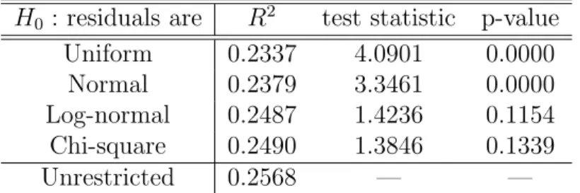
As discussed in Section 6.2, formal hypothesis testing is straightforward, requiring a mere linear restriction test on the coefficients of a linear regression Table 2 presents the results of this test for each distribution.15 The
conclu-sions coincide roughly with the ones reached informally with the graphs: the hypotheses of uniform or normal residuals are rejected at conventional significance levels.
H0 : residuals are R2 test statistic p-value
Uniform 0.2337 4.0901 0.0000
Normal 0.2379 3.3461 0.0000
Log-normal 0.2487 1.4236 0.1154
Chi-square 0.2490 1.3846 0.1339
Unrestricted 0.2568 — —
Table 2: Hypothesis testing on the distribution of residuals.
7.1
Testing for Gaussian Common Values
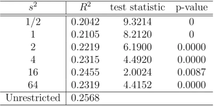
Tests have also been run for the hypothesis that the true data generating process is an English common value auction with distributional assumptions as in appendix A. Tests have been run for s2 = 1/2, 1, 2, 4, 16 and 64.16
The results reported on table 3 show that all of the affiliated models tested have been rejected. The results therefore do not provide evidence against the independent private values assumption in this sample. One must keep in mind, however, that these are tests on specific affiliated models. They provide no indication on whether some other affiliated model is rejected.
15The test statistic is the F-test based on R2 differences, for the hypothesis that the
estimated dummies for ˆa(2) to ˆa(20) is equal to the numbers in each column of table 1, up to scale and location. Here the degrees of freedom are 57−30 = 17 and 2299−57 = 2242.
s2 R2 test statistic p-value
1/2 0.2042 9.3214 0
1 0.2105 8.2120 0
2 0.2219 6.1900 0.0000
4 0.2315 4.4920 0.0000
16 0.2455 2.0024 0.0087
64 0.2319 4.4152 0.0000
Unrestricted 0.2568
Table 3: Hypothesis testing, Gaussian Common Values.
8
Concluding Remarks
This paper proposes a method that combines the strenghts of two distincts branches of the auction econometrics literature, being at once computation-ally accessible and theoreticcomputation-ally sound. It is also robust in a wide variety of contexts.
In a nutshell, the main finding of the paper is that one can estimate parameters that affect the location and scale of the value distribution in a simple and unbiased way, provided one controls for variables that affect bid-ding behavior in a flexible way. Under symmetry, the main such variable is the number of participating bidders (equation 4); in more complex asymmet-ric situations, it is the number of bidders of each given type (equation 5); similarly, the discussion in section 5.3.2 suggest that when entry is a concern, the appropriate regression would include a correction parameter that depends on instruments correlated with the entry decision process (equation 8).
As such, the method provides a simple way to separate the effect of regres-sors that affect bidding only by affecting the value distribution from those that affect bidding strategically. It provides an useful tool for researchers interested in measuring the former while properly controlling for the latter; conversely, it helps identify the misspecification bias that occurs when the latter are not accounted for.
auc-tion data.
A
Examples with Affiliation
This section provides examples of the methodology applied to the context of the affiliated model of Milgrom and Weber (1982). In this model, the value of the item for each bidder is no longer private and independent; it is rather a function of a number of affiliated random variables. Vil, the value of the
item for bidder iin auction l, is
Vil =Vl(Sil, S−li, S
l
0),
where Sl
i is the signal of bidder i in auction l, S−li is the vector of signals
of the other bidders, and Sl
0 is an additional random variable or vector not
observed by any bidder. Each bidder j observes Sl
j prior to the auction, but
not Vjl. S0l, . . . , Snl are affiliated, and Vl is increasing in all arguments.
We parameterize the model in a way analogous to Assumption 1:
Assumption 5 Vil =µl+σlνil, where νil =ν(Sil, S−li, S
l
0). The distribution
of (Sl
0, . . . , Snl) is i.i.d. across auctions, and ν is the same across auctions.
As before, all variation across auctions is captured by the mean and the variance of the valuations. Signals and values are allowed to exhibit fairly complex dependencies within an auction, but once one normalize the values, one obtains a random sample of auctions.
One feature that is lost once we move away from the independent private values framework in the Expected Revenue Equivalence Theorem. Now the expected price for the good will depend on the specific auction format to be used. Following Milgrom and Weber (1982), we discuss three possible auction formats: the second-price or Vickrey auction, the English auction, and the first-price auction. We distinguish bid functions and resulting prices across these auctions using superscripts V, E and F, respectively. Milgrom and Weber (1982) have provided characterizations for equilibria in each of the three alternative mechanisms.
In the Vickrey auction l, it is an equilibrium to bid according to
wherebV
l (s) represents the bid of bidderiwhen it observes a signals.
Assum-ingbV is increasing, and since the affiliated model is symmetric, the winner is
the bidder with the highest signal, and the final price will bepV =bV(Sl
(2:nl)).
Using assumptions 2 and 5, we can write the expected price as follows:
E[pVl |Xl, Zl, nl] = E[blV(S(2:l nl))|Xl, Zl, nl]
= E[E[Vil|Sil =S(2:nl)l, S
l
(1:nl)=S
l
(2:nl)]|Xl, Zl, nl]
= E[E[µl+σlνi|Sil =S(2:nl)l, S
l
(1:nl)=S
l
(2:nl)]|Xl, Zl, nl]
= µl+σlE[νi|Sil =S(1:nl)l =S
l
(2:nl)],
where the second equality comes from the equlibrium bidding function, the third from the specification of Vil, and the fourth from linearity of the
con-ditional expectation operator. Defining aV(n) = E[ν
i|Sil = S(2:l n), S(1:l n) =
Sl
(2:n)], we have
E[pVl |Xl, Zl, nl] = Xlβ+aV(nl)Zlα. (9)
As in equation 3, the conditional expectation of the price is linear, and OLS provides unbiased and consistent estimates. Both methods 1 and 2 can again be used; the only change in method 1 needed to accommodate affiliation would be to calculate aV(n) = E[νi|Sil = S(2:l n), S(1:l n) = S(2:l n)]
instead of a(n) =E[ǫ(2:n)]. Method 2 does not require any change.
The same result obtains in the English auction. In that case, a bid func-tion must specify a drop-out point for each signal and each history of drop-out points by the opponents. LetbE
l (s,∅) is the drop-out point of a bidder with
signal s who has not seen anybody drop out, and bE
l (s,(d1, . . . , dk)) is the
one for a bidder that has observed a history (d1, . . . , dk) of drop-out points.
Milgrom and Weber (1982) characterize an equilibrium to this game re-cursively as follows:
bEl (s,∅) = E[Vil|Sl
i =s, S−li(1) =· · ·=S
l
−i(n−1) =s],
bEl (s,(d1)) = E[Vil|Sil=s, S−li(1) =· · ·=S
l
−i(n−2) =s, b
E
l (S−li(n−1),
∅) = d1],
bEl (s,(d1, d2)) = E[Vil|Sil=s, S−li(1) =· · ·=S
l
−i(n−3) =s, b
E
l (S−li(n−2),(d1)) = d2,
bE
l (S−li(n−1),
Assuming that these functions are one-to-one on s, one can infer the signal of each losing bidder from their drop-out points. The auction price, the drop-out point of the final losing bidder, is
pE =E[V(2:nl)l|S
l
(1) =S(2)l , S(2)l , . . . , S(ln)],
that is, the estimated value for this bidder if we know the signals of all losers and assume the winner has the same signal as the last loser.
Since the price is still a conditional expectation, linearity holds in this case as well. We obtain
E[pEl |Xl, Zl, nl] = Xlβ+aE(nl)Zlα, (10)
where this time aE(n) = E[E[ν
i|Sil =S(2)l , S(1:l n) = S(2:l n), S(2)l , . . . , S(ln)]]. So
again method 1 is applicable using this espression for a(n), and method 2 is applicable unchanged.
We now turn to the case of a first-price auction. Milgrom and Weber (1982) show that in a symmetric equilibrium of this game the bid function is
bF(s) =
Z s
bV(t)dL(t|s),
where
L(t|s) = exp
−
Z s
t
h(y|y)dy
,
and h(x|y) is the hazard rate of the opponents’ highest signal, conditional on an individual’s signal. Observe that Lis a function of the signal structure of the model only, and not of the value function. So it does not change across auctions.
So we can write
bF(s) =
Z s
E[µl+σlνi|Sil =t,max(S−li) =t]dL(t|s)
= µl+σl
Z s
E[νi|Sil =t,max(S−li) =t]dL(t|s),
and therefore the expected price is
E[pFl |Xl, Zl, nl] = Xlβ+aF(nl)Zlα, (11)
In all three cases the methodology suggested works. Unbiased, consistent estimates of the coefficients that determine the expectation and variance of the valuations can be obtained by OLS even in the more general affiliated framework. In order to apply method 1 the only necessary modification is to redefine the artificial regressor a(n) in a way that depends on the specific auction rule. For method 2, no changes are necessary.
We now provide artificial regressors ˜a(n) for a particular example of an affiliated model: a case where agents have a common value for the object, and only differ because they observe different signals of that value.
In order to obtain specific figures for ˜a(n), we assumeVil =Vl∼ N(µl, σ2l)
is common across bidders within an auction. Let vl = (Vl −µl)/σl be the
normalized value. Bidders observe different signals Sl
i, with Sil = vl +ǫil,
with disturbances ǫil ∼ N(Vl, s2) independent of each other and vl.
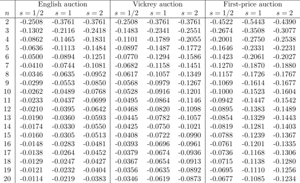
This model is a special case of the affiliated model, known in the literature as the common-values or mineral rights model. Here we allow for variation in the mean and variance of the valuations across auctions as before. We impose a specific distributional assumption for valuations and signals in order to compute artificial regressors.17
Artificial regressors have been computed for the English auction, the Vick-rey auction and for the First-price auction, for all numbers of bidders between 2 and 20. They are reported in Table 4. Three values for the variance of the signal error have been used: 0.5, 1 and 2. Since the variance of the nor-malized value is 1, these choices represent the cases where uncertainty about signal errors is smaller than, equal, or greater than uncertainty about the value.
B
Proofs
Proof of lemma 1: Sinceω(k:n)= (k−1)!(n!n−k)! R
vF(v)n−k
(1−F(v))k−1
dF(v), we have that
nω(k:n−1) =
n! (k−1)!(n−1−k)!
R
vFn−1−k
(1−F)k−1
dF(v)
= n!
(k−1)!(n−1−k)! R
vFn−1−k
(1−F)k−1
[F + (1−F)]dF(v)
17We truncate the distributions of normalized values at the interval [-10,10]. This is
English auction Vickrey auction First-price auction
n s= 1/2 s= 1 s= 2 s= 1/2 s= 1 s= 2 s= 1/2 s= 1 s= 2 2 -0.2508 -0.3761 -0.3761 -0.2508 -0.3761 -0.3761 -0.4522 -0.5443 -0.4390 3 -0.1302 -0.2116 -0.2418 -0.1483 -0.2341 -0.2551 -0.2674 -0.3508 -0.3077 4 -0.0862 -0.1465 -0.1831 -0.1101 -0.1789 -0.2055 -0.2001 -0.2750 -0.2538 5 -0.0636 -0.1113 -0.1484 -0.0897 -0.1487 -0.1772 -0.1646 -0.2331 -0.2231 6 -0.0500 -0.0894 -0.1251 -0.0770 -0.1294 -0.1586 -0.1423 -0.2061 -0.2027 7 -0.0410 -0.0744 -0.1081 -0.0682 -0.1158 -0.1451 -0.1270 -0.1870 -0.1880 8 -0.0346 -0.0635 -0.0952 -0.0617 -0.1057 -0.1349 -0.1157 -0.1726 -0.1767 9 -0.0299 -0.0553 -0.0850 -0.0568 -0.0979 -0.1267 -0.1069 -0.1614 -0.1677 10 -0.0262 -0.0489 -0.0768 -0.0528 -0.0916 -0.1201 -0.1000 -0.1523 -0.1604 11 -0.0233 -0.0437 -0.0699 -0.0495 -0.0864 -0.1146 -0.0942 -0.1447 -0.1542 12 -0.0210 -0.0395 -0.0642 -0.0468 -0.0820 -0.1098 -0.0895 -0.1383 -0.1489 13 -0.0190 -0.0360 -0.0593 -0.0445 -0.0782 -0.1057 -0.0854 -0.1329 -0.1443 14 -0.0174 -0.0330 -0.0550 -0.0425 -0.0750 -0.1021 -0.0819 -0.1281 -0.1403 15 -0.0160 -0.0305 -0.0513 -0.0408 -0.0722 -0.0990 -0.0788 -0.1239 -0.1367 16 -0.0148 -0.0283 -0.0481 -0.0393 -0.0696 -0.0961 -0.0761 -0.1201 -0.1335 17 -0.0138 -0.0264 -0.0452 -0.0379 -0.0674 -0.0936 -0.0736 -0.1168 -0.1306 18 -0.0129 -0.0247 -0.0427 -0.0367 -0.0654 -0.0913 -0.0715 -0.1138 -0.1280 19 -0.0121 -0.0232 -0.0404 -0.0356 -0.0635 -0.0892 -0.0695 -0.1110 -0.1256 20 -0.0114 -0.0219 -0.0383 -0.0346 -0.0619 -0.0873 -0.0677 -0.1085 -0.1234
= n! (k−1)!(n−1−k)!
R
vFn−k
(1−F)k−1
dF(v)
+(k−1)!(nn!−1−k)! R
vFn−1−k
(1−F)kdF(v)
= (n−k)ω(k:n)+kω(k+1:n)
so the recurrence relation holds.
Proof of corollary 1: By induction, since it is immediate that with all
ω(k:n) and a(n+ 1), one can directly compute all remaining ω(k:n+1).
Proof of lemma 2: The argument roughly follows Hoeffding (1953). We
will show that the distribution of ǫ(kn,n) converges to the constant F
−1
(α). Given a quantileu, Pr(ǫ(kn,n) < F
−1
(u)) can be written as
Ru
0(1−t)
kn
tn−kn
dt
R1
0(1−t)k
ntn−kndt
.
We must show that this goes to 0 for u < α and to 1 for u > α.
Take u < α. Fixv ∈(u, α). For a sufficiently high n, αn = 1−kn/n > v.
The function tαn
(1−t)1−αn
is increasing for t < αn; so
Ru 0 [t
αn
(1−t)1−αn
]ndt
R1 0[tα
n(1−t)1−αn]ndt ≤
Ru 0 [t
αn
(1−t)1−αn
]ndt
Rαn
v [tα
n(1−t)1−αn]ndt ≤ Ru
0 [uα
n
(1−u)1−αn
]ndt
Rαn
v [vα
n(1−v)1−αn]ndt =
u αn−v
uαn
(1−u)1−αn
vαn(1−v)1−αn n
→ 0.
The argument for u > α is analogous, since the function tαn
(1−t)1−αn
is decreasing for t > αn.
References
Amemiya, Y. (1985): “Instrumental Variable Estimator for the Nonlinear Errors-in-Variables Model,” Journal of Econometrics, 28(3), 273–289.
Athey, S., and P. A. Haile (2002): “Identification of Standard Auction
Models,” Econometrica, 70(6), 2107–2140.
Bajari, P., and A. Hortac¸su (2003): “The Winner’s Curse, Reserve
Prices, and Endogenous Entry: Empirical Insights from eBay Auctions,” RAND Journal of Economics, 34(2).
Bikhchandani, S., P. A. Haile, and J. G. Riley (2002): “Symmetric
Separating Equilibria in English Auctions,”Games and Economic Behav-ior, 38, 19–27.
Campo, S., I. Perrigne, and Q. Vuong (2001): “Assymetry in
First-Price Auctions with Affiliate Private Values,” USC. forthcoming in the Journal of Applied Econometrics. .
Chan, L. K. (1967): “On a Characterization of Distribution by Expected Values of Extreme Order Statistics,” American Mathematics Monthly, 74, 950–951.
Deltas, G., and I. Chakraborty (2001): “Robust Paratric Analysis of
First Price Auctions,” University of Illinois and University of Oklahoma..
Donald, S. G., and H. J. Paarsch(1993): “Piecewise Pseudo-Maximum
Likelihood Estimation in Empirical Models of Auctions,” International Economic Review, 34(1), 121–148.
Garcia, M., and L. Rezende (2000): “Short-Term Security Auctions by
Brazilian Central Bank: Study of Conditioning Factors of Dispersion of the Bids,” Brazilian Journal of Political Economy, 20(4), 8–25, (in Por-tuguese).
Gilley, O. W., and G. V. Karels (1981): “The Competitive Effect in Bonus Bidding: New Evidence,” Bell Journal of Economics, 12(2), 637– 648, .
Guerre, E., I. Perrigne, and Q. Vuong (2000): “Optimal
Nonpara-metric Estimation of First-Price Auctions,”Econometrica, 68(3), 525–574.
Haile, P., H. Hong, and M. Shum (2003): “Nonparametric Tests for
Common Values in First-Price Sealed-Bid Auctions,” .
Haile, P., and E. Tamer(2003): “Inference with an Incomplete Model of
Hoeffding, W. (1953): “On the Distribution of the Expected Values of the Order Statistics,” Annals of Mathematical Statistics, 24, 93–100.
Hong, H., and E. Tamer (2003): “A simple estimator for nonlinear error
in variable models,” Journal of Econometrics, 117(1), 1–19.
Houser, D., and J. Wooders (2000): “Reputation in Auctions: Theory,
and Evidence from eBay,” University of Arizona.
Krasnokutskaya, E. (2002): “Identification and Estimation in Highway Procurement Auctions under Unobserved Auction Heteogeneity,” Yale.
Laffont, J.-J., H. Ossard, and Q. Vuong (1995): “Econometrics of First-Price Auctions,” Econometrica, 63(4), 953–980.
Laffont, J.-J., and Q. Vuong (1996): “Structural Analysis of Auction
Data,”American Economic Review, 86(2), 414–420.
Lebrun, B. (1996): “Existence of Equilibrium in First Price Auctions,” Economic Theory, 7, 421–443.
Lee, L.-F., and J. H. Sepanski(1995): “Estimation of Linear and
Non-linear Error-in-Variables Models Using Validation Data,” Journal of the American Economic Association, 90(429), 130–140.
Levin, D., andJ. L. Smith(1994): “Equilibruim in Auctions with Entry,”
American Economic Review, 84(3), 585–599.
Lucking-Reiley, D., D. Bryan, N. Prasad, and D. Reeves (2000):
“Pennies from eBay: the Determinant of Price in Online Auctions,” Uni-versity of Arizona.
McAfee, R. P., and J. McMillan (1987a): “Auctions with a Stochastic
Number of Bidders,”Journal of Economic Theory, 43(1), 1–19.
(1987b): “Auctions with Entry,”Economics Letters, 23(4), 343–347.
McDonald, C. G., and V. C. Slawson (2002): “Reputation in an In-ternet Auction Market,” Economic Inquiry, 40(4), 633–50.
Melnik, M. I., and J. Alm (2002): “Does a Seller’s Ecommerce
Milgrom, P. R., and R. J. Weber (1982): “A Theory of Auctions and
Competitive Bidding,”Econometrica, 50(5), 1089–1122.
Myerson, R. B. (1981): “Optimal Auction Design,” Mathematics of Op-erations Research, 6(1), 58–73.
Newey, W. K. (2001): “Flexible Simulated Moment Estimation of Non-linear Errors-in-Variables Models,” Review of Economics and Statistics, 83(4), 616–627.
Olley, G. S., and A. Pakes (1996): “The Dynamics of Productivity in the Telecommunications Equipment Industry,”Econometrica, 64(6), 1263– 1297, .
Paarsch, H. J. (1991): “Empirical Models of Auctions and an Applica-tion to British Columbian Timber,” Research Report 9212, University of Western Ontario Department of Economics.
Pollak, M. (1973): “On Equal Distributions,”Annals of Statistics, 1, 180– 182.
Samuelson, W. F. (1985): “Competitive bidding with entry costs,” Eco-nomics Letters, 17(1-2), 53–57, .
regressor coef. st.dev. regr. coef. st.dev. regr. coef. st.dev. broken -106.66 28.70 21 198.53 14.39 42 212.50 102.50 2 58.82 7.93 22 220.01 12.91 43 292.50 72.48 3 59.63 8.63 23 217.47 14.21 44 293.35 59.17 4 91.68 9.81 24 218.39 13.94 45 300.00 102.50 5 109.82 10.68 25 221.85 14.49 46 322.00 102.50 6 109.99 10.68 26 219.85 14.07 47 310.00 102.50 7 136.57 10.74 27 226.79 17.32 48 167.50 102.50 8 145.31 11.32 28 242.82 19.03 53 305.00 102.50 9 182.05 10.93 29 242.71 18.71 58 222.50 102.50 10 139.77 10.64 30 236.44 17.57 64 281.00 102.50 11 160.15 11.46 31 233.96 20.50 67 225.00 102.50 12 162.11 10.06 32 228.80 26.46 90 291.00 102.50 13 184.43 10.63 33 246.58 29.58 93 205.00 102.50 14 199.03 12.08 34 239.61 28.42 106 280.00 102.50 15 198.21 11.99 35 172.84 34.16 126 285.50 102.50 16 187.46 12.61 36 182.14 38.74 128 215.50 102.50 17 214.40 13.23 37 242.10 45.84 134 280.00 102.50 18 217.64 11.68 38 190.00 51.25
19 228.21 10.92 39 206.25 51.25 20 204.15 12.92 40 278.50 59.17
uniform normal lognormal chi-square regressor coef. st.dev. coef. st.dev. coef. st.dev. coef. st.dev.
broken -109.98 28.94 -109.45 28.86 -108.00 28.65 -108.50 28.65 intercept 77.72 4.17 79.48 4.05 93.45 3.45 90.65 3.54
slope 78.06 3.83 81.53 3.93 95.45 4.41 81.25 3.75 21 120.94 15.14 119.16 15.07 105.13 14.82 107.95 14.84 22 142.29 13.71 140.53 13.64 126.56 13.38 129.35 13.41 23 139.75 14.97 137.98 14.90 124.02 14.65 126.81 14.67 24 140.67 14.71 138.91 14.64 124.94 14.39 127.73 14.41 25 144.13 15.24 142.37 15.17 128.40 14.92 131.19 14.94 26 142.13 14.84 140.37 14.77 126.40 14.51 129.20 14.53 27 149.07 18.01 147.31 17.94 133.34 17.69 136.14 17.71 28 165.10 19.70 163.34 19.62 149.37 19.37 152.17 19.38 29 164.99 19.38 163.23 19.30 149.26 19.06 152.05 19.07 30 158.71 18.26 156.95 18.19 142.99 17.94 145.78 17.95 31 156.24 21.15 154.47 21.07 140.51 20.82 143.30 20.83 32 151.07 27.09 149.31 27.00 135.35 26.73 138.14 26.74 33 168.86 30.22 167.09 30.12 153.13 29.83 155.92 29.84 34 161.89 29.05 160.13 28.96 146.16 28.68 148.95 28.69 35 95.12 34.81 93.36 34.70 79.39 34.39 82.18 34.40 36 104.42 39.41 102.65 39.29 88.69 38.95 91.48 38.96 37 164.37 46.55 162.61 46.42 148.64 46.04 151.44 46.04 38 112.27 52.01 110.51 51.86 96.54 51.44 99.34 51.44 39 128.53 52.01 126.76 51.86 112.80 51.44 115.59 51.44 40 200.78 60.00 199.01 59.83 185.05 59.37 187.84 59.37
bids auctions bids auctions bids auctions
2 167 21 51 40 3
3 141 22 63 42 1
4 109 23 52 43 2
5 92 24 54 44 3
6 92 25 50 45 1
7 91 26 53 46 1
8 82 27 35 47 1
9 88 28 29 48 1
10 93 29 30 53 1
11 80 30 34 58 1
12 104 31 25 64 1
13 93 32 15 67 1
14 72 33 12 90 1
15 73 34 13 93 1
16 66 35 9 106 1
17 60 36 7 126 1
18 77 37 5 128 1
19 88 38 4 134 1
20 63 39 4