DOI: 10.1590/1808-057x201806870
*Paper presented at the XVII International Conference in Accounting, São Paulo, SP, Brazil, July 2017.
**The authors are grateful for the financial support received from the Brazilian National Council for Scientific and Technological Development (CNPq) and for the comments and time dedicated by the ad hoc reviewers, which led to improvements in this study.
Original Article
Business cycles and earnings management strategies: a study in
Brazilian public firms*
,**
Edilson Paulo1
https://orcid.org/0000-0003-4856-9039 Email: edilson.paulo@ufrgs.br
Renato Henrique Gurgel Mota2
https://orcid.org/0000-0001-8439-7540 Email: renatogurgel@ufersa.edu.br
1 Universidade Federal do Rio Grande do Sul, Faculdade de Ciências Econômicas, Departamento de Ciências Contábeis e Atuariais, Porto Alegre, RS, Brazil
2 Universidade Federal Rural do Semi-Árido, Centro de Ciências Sociais Aplicadas e Humanas, Departamento de Ciências Sociais Aplicadas, Mossoró, RN, Brazil
Received on 10.30.2017 – Desk acceptance on 11.30.2017 – 4th version approved on 06.13.2018
Associate Editor: Eliseu Martins
ABSTRACT
This study contributes to the literature dealing with the influence of macroeconomic factors on accounting information quality, since it analyzes the earnings management strategies of firms, specifically identifying different discretionary behaviors among economic cycles: 1) different levels of earnings management through accruals between phases of the business cycle, and 2) the trade-off between earnings management through accruals and real earnings management. The results indicate that the accounting information reported should be analyzed with greater caution by its users, especially in periods of great economic oscillations, when managers can increase or reduce opportunistic behavior. The research population comprised non-financial companies with shares traded on the São Paulo Stock, Commodities, and Futures Exchange (BM&FBovespa) and the sample was composed of 247 firms per year, covering the period from 2000 to 2015 and totaling 2,501 observations. The phases of business cycles were used as a proxy for the economic environment and were based on Schumpeter’s (1939) study, which divides an business cycle into four distinct phases: expansion, recession, contraction, and recovery. Discretionary accruals were estimated according to the Pae (2005) and Paulo (2007) models. Real earnings management was estimated as described by Roychowdhury (2006), using only the abnormal behavior of production costs and operational decisions. The results of this research show that earnings management strategies, using either accruals or real manipulation, as well as the choice between these strategies, are impacted by the economic environment. The evidence suggests that managers have different opportunistic behavior in each phase of the business cycle. Specifically, they increase the level of discretionary accruals in contractionary phases and reduce it during recoveries, while they manage earnings downwards via real manipulation in recessions and contractions.
Keywords: business cycles, financial crisis, earnings management, accounting information quality.
Correspondence address
Edilson Paulo
Universidade Federal do Rio Grande do Sul, Faculdade de Ciências Econômicas, Departamento de Ciências Contábeis e Atuariais Avenida João Pessoa, 52 – CEP 90040-060
1. INTRODUCTION
The impact on the capital market of the publication of firms’ accounting information has been evidenced since the seminal studies by Ball and Brown (1968) and Beaver (1968). However, Lev (1989) claims that studies have shown a weakening in the association between return and accounting earnings caused by the arbitrariness of the accounting measures and by earnings manipulations by managers, thus affecting accounting information quality.
By analyzing earnings management (EM) behavior in various countries facing financial crises, studies have shown that accounting information quality can also be impacted by macroeconomic issues. Research has revealed that opportunistic behavior on the part of managers decreases in times of financial crises (Filip & Raffournier, 2014; Kousenidis, Ladas & Negakis, 2013). This may occur due to the restricted ability of companies to manage earnings through accruals. According to Filip and Raffournier (2014), companies with high levels of accruals engaged more in income smoothing in crisis periods, unlike those with low levels of accruals, which reduced income smoothing in these periods.
However, the literature also reports an increase in EM practices in times of crises (Iatridis & Dimitras, 2013; Persakis & Iatridis, 2015; Tahinakis, 2014; Trombetta & Imperatore, 2014). This inconsistency in the findings of previous studies may derive from the existence of a trade-off between accruals-based earnings management (AEM) and real earnings management (REM), depending on the costs associated with each EM strategy (Zang, 2012).
Previous studies on financial crises have only analyzed one of the earnings management strategies, that is, the use of accruals. However, Cohen and Zarowin (2010) reinforce the importance of analyzing both EM strategies available to managers, given that AEM does not have direct consequences on cash flow, unlike REM.
Furthermore, the studies that address EM and the impact of the economic environment have only done so by analyzing periods of financial crises. In contrast, this study aims to analyze this relationship by adopting the four phases of business cycles as a proxy for fluctuations in the economic environment. Schumpeter (1939) and Burns and Mitchell (1946) describe economic or business cycles as fluctuations found in the overall economic activity of countries that organize their work, especially in corporate business. According to the authors, a business cycle consists
of four phases: expansion, which occurs almost at the same time in many economic activities, similarly followed by general recession, contraction, and recovery, which merge with the expansionary phase of the following cycle.
Therefore, in this study, we aimed to analyze two points that have not yet been explored by the current literature concerning the relationship between EM strategies and economic cycles:
1. Accruals-based earnings management in the different phases of the business cycle: discretionary behavior in relation to accruals can be influenced by the business cycle in which the firm finds itself. For example, in an expansion or a recovery, manages may be more prone to reporting more positive company earnings than in the others (income maximization) or to exceeding market analysts’ expectations. In contrast, in periods of contraction or recession, they may report lower results, using discretion regarding accruals so that these are reversed in the following periods, thus improving their future results (big bath).
2. Trade-off between AEM and REM: in light of the restrictions on the use of discretionary behavior regarding accruals, managers may alter their EM strategy in order to serve their own personal interests or those of the firm. In addition, in times of business crises, for example, it is common for managers to “cut” costs in the company in order to improve their results at the end of the period.
Thus, in light of the indications regarding the influence of the economic environment on accounting information quality (Filip & Raffournier, 2014; Iatridis & Dimitras, 2013; Persakis & Iatridis, 2015) and of the possible relationships between EM strategies and the economic environment, we are presented with the following research problem: what is the influence of business cycles over the earnings management strategies used by publicly-traded Brazilian companies?
determined based of the studies by Schumpeter (1939) and Burns and Mitchell (1946) were used as a proxy.
According to Zang (2012), as previously presented, there are a number of restrictions and incentives associated with the earnings manipulations that managers are willing to engage in. For example, achieving the earnings predicted by market analysts using EM can compromise the accounting earnings of the following period. Therefore, depending on the phase in which the economy finds itself, managers may be more or less likely to engage in EM. However, this can differ according to the macroeconomic factors in which firms operate. Thus, this study could help investors, creditors, and regulatory bodies in their decision-making when faced with the fluctuations in the economic activity that occur in Brazil.
The relationship proposed in this study is a subject that has been scarcely explored by the literature. Some studies have only included gross domestic product (GDP) to control for the effect of fluctuations in economic activity on the proxies for earnings management (Cohen & Zarowin, 2010; Zang, 2012) or they have separated economic fluctuations into only two phases: expansion and recession (Dimitras, Kyriakou & Iatridis, 2015; Jenkins, Kane & Velury, 2009; Jiang, Habib & Gong, 2015), as reported by the National Bureau of
Economic Research (NBER). However, according to Schumpeter (1939), the studies based only on the phases of contraction and expansion do not investigate smaller oscillations, such as recession and contraction. In comparison terms, the NBER’s “contraction” phase is divided into the contraction and recession phases, and the “expansion” phase is composed of recovery and expansion, according to the classification by Schumpeter (1939) and Burns and Mitchell (1946).
In the specific case of REM, Kim and Sohn (2013) argue that due to the impact on cash flow resulting from the use of this strategy, the quality of earnings information used by investors is also reduced, thus requiring a higher risk premium for companies that manipulate their earnings. Therefore, this study is also warranted due to the use of accounting information by the capital market, since an adequate understanding of the opportunistic behavior of managers in the event of changes in the country’s economy could help in decision making regarding the allocation of the resources available to investors, for example by contributing to an improvement in financial analysts’ forecasts or to adequate credit risk analysis in view of the different discretionary behaviors depending on the phase of the business cycle.
2. THEORETICAL FRAMEWORK
Business cycles originate from fluctuations in the level of a country’s economic activity, generally measured by GDP. The NBER, the US body responsible for identifying business cycles, divides one full cycle into two phases: recession and expansion. For the NBER, recession occurs when there are two or more consecutive quarters of negative GDP, while expansion occurs when there are two or more consecutive quarters of GDP growth (Knopp, 2010). Cycles are measured based on peaks and troughs. For example, the peak of an expansion is the point in time at which the level of GDP reaches its maximum before beginning to decline. Thus, the peak of an expansion marks the start of a recession. Similarly, the trough of a recession is the moment at which GDP has fallen to its lowest level before beginning to rise again, which means that a trough marks the start of an expansion (Knopp, 2010).
Schumpeter (1939) defends a four-stage cyclical process, which presents growth in economic activity in the recovery and expansion phases, with a reduction in this activity
occurring in the recession and depression phases. The author refers to the concept of equilibrium state. Although this state can never actually occur, he claims that it is valid solely as a reference point, since various events (political, cultural, natural, etc.) collide with the economic world, which is already disturbed and unbalanced. In Schumpeter’s (1939) view, there is a tendency to equilibrium, which after each excursion draws the system back towards a new equilibrium state. The author also notes that this tendency is caused by a real force (innovations) and not by the mere existence of ideal equilibrium points of reference. In support, Burns and Mitchell (1946) also classify business cycles into four distinct phases: expansion, recession, contraction, and recovery.
Filip & Raffournier, 2014; Kousenidis et al., 2013; Persakis & Iatridis, 2015) or by using the binary classification published by the NBER (Dimitras et al., 2015; Jenkins et al., 2009; Jiang et al., 2015). Unlike previous papers, this one has conducted the study by considering the four phases of business cycles.
According to Schipper (1989), earnings management is related to disclosure management, that is, a deliberate intervention in the process of externally disclosing financial information with the intention of achieving some particular gain. Similarly, for Healy and Wahlen (1999), earnings management occurs when managers use their judgment in financial reports to structure operations with the aim of misleading some parties interested in the company’s underlying economic performance or in order to influence the contractual results that depend on the accounting numbers reported.
In a study carried out involving companies in the
European stock market, Dimitras et al. (2015) examined the
consequences of the European financial crisis in relation to earnings management and found that companies tend to reduce earnings management practices in times of crisis. However, the authors warn that the results may depend on specific aspects of each country’s economic environment.
Kousenidis et al. (2013) sought to determine
whether, and to what extent, the crisis in the European Union had an impact on the earnings quality of listed companies in countries with weak fiscal sustainability. The results of this study indicate that, on average, the accounting information quality improved. During the crisis period, companies appear to report more timely, more conservative, more relevant, less smoothed, less managed, more persistent, and more predictable earnings. However, these results are slightly different for those companies that have the greatest absolute discretionary accruals in the crisis period. Borio (2014) reports that, despite the financial cycle being longer than the business cycle, financial crises are also generally accompanied by the recessionary phase of the business cycle.
Therefore, in light of the absence of studies on the relationship between the level of earnings management and the four phases of business cycles and the evidence from previous studies on financial crises presenting indications that the level of earnings management may be associated with the phases of business cycles, we are presented with the following research hypothesis:
H1: discretionary behavior in relation to the accounting choices
(accruals) of publicly-traded Brazilian companies is influenced by the country’s business cycle.
However, earnings management can occur via both accruals and operational decisions. According to Zang (2012), the decision regarding the type of management managers are willing to engage in depends on the cost associated with each one. The author also claims that managers use AEM or REM as substitutes; that is, managers adjust the level of discretionary accruals in accordance with the level of REM.
Cohen and Zarowin (2010) claim that managers alternate between both EM methods based on their relative costs, and that the level of accruals for the period is adjusted according to the level of REM carried out in the year. This study showed that companies that have issued shares in the market manage their earnings both via accruals and via REM, and that reduced earnings are more associated with REM than with accruals. Gunny (2010) considers that REM has greater costs for managers since, unlike accruals, they have direct consequences on cash flow and can therefore have a damaging economic impact on the firm’s value in the long term.
In light of the evidence of changes in earnings management strategy between AEM and REM and of changes in discretionary behavior depending on the phases of the business cycle, we have the second research hypothesis:
3. METHODOLOGICAL PROCEDURES
3.1. Population and Sample
The sample in the study derives from the population of public companies with shares traded on the São Paulo Stock, Commodities, and Futures Exchange (BM&FBovespa) between 2000 and 2015. This population was chosen due to the obligation to publish annual accounting statements, as well as due to it being composed of companies from various sectors of economic activity. The accounting data used in this study to calculate discretionary accruals and real earnings management were collected from the
Bloomberg® database. To compose the research sample,
financial institutions and insurers were excluded, as these companies have a different ownership and operational
structure and they also present a high degree of leverage that can distort the calculation of the variables used by the earnings management estimation models. In addition, observations with some incomplete field and outliers identified via boxplot analysis were excluded. Table 1 describes the composition of the sample.
The sectors were grouped according to the classification
of the Bloomberg® database using the Industry
Classification Benchmark (ICB) methodology. As Table 1 shows, the sample is composed of 14 sectors, of which the Public Utility and Telecommunications, Personal and Domestic Products, and Industrial Goods and Services sectors warrant mentioning for having a greater number of both firms and observations per sector.
Table 1
Description of the research sample covering 2000 to 2015
Description Quantity
Companies Observations
Number of non-financial firms in
the Brazilian stock market 278 4,448
Data missing for the calculation of the variables 20 1,991
Observations considered outliers 11 44
Research sample (companies per year) 247 2,501
Sector
Health 5 61
Oil and Gas 5 50
Technology 5 73
Vehicles and Autoparts 7 76
Travel and Leisure 7 72
Chemical Products 9 100
Building Materials 13 124
Basic Resources 18 221
Real Estate 18 179
Food and Drink 20 153
Retail 23 218
Industrial Products and Services 32 314
Personal and Domestic Products 37 388
Public Utility and Communications 48 472
Source: Elaborated by the authors.
The analysis period is warranted due to the fact that it covers moments of economic-financial crises, as well as times of expansion in the Brazilian economy. Figure 1 presents the percentage variation in quarterly Brazilian
GDP between the 1st quarter of 1999 and the 2nd quarter
of 2015.
In Figure 1, it is possible to note periods followed by positive variations in GDP between 2002 and 2008,
Figure 1
Percentage variation in gross domestic product (GDP) by quarter in relation to the previous quarter – 2000 to 2015 Source: Bloomberg®, 2016.
Therefore, the period analyzed is marked by both reductions and growth in GDP, thus forming the fluctuations that give rise to the business cycles that occurred in Brazil.
3.2. Research Variables
The business cycles were divided into four phases (expansion, recession, contraction, and recovery) identified in accordance with Schumpeter (1939). The mean of the real variations in GDP was treated as tendency to equilibrium, based on which the expansion and recession phases were separated from the contraction and recovery phases. Two quarters before and after the
study period were added to enable a full analysis of the period studied.
So, starting from an expansion, GDP varies positively and above the mean. During recession, there continues to be above-average growth, but with negative variations. During contraction, the economy heads towards a recession – contraction of the economy for two or more consecutive quarters – with GDP variations being negative and below average. It is during recovery that the economy returns to growth, with positive variations in real GDP, but still below tendency to equilibrium, until the next phase, which begins a new cycle starting with the expansionary phase. The classification of the phases is shown in Figure 2.
Figure 2
Phases of a business cycle according to Schumpeter (1939) GDP = gross domestic product
Source: Elaborated by the authors.
-8 -6 -4 -2 0 2 4 6 8 10 06 /30 /20 16 09 /30 /20 15 12 /31 /20 14 03 /31 /20 14 06 /30 /20 13 09 /30 /20 12 12 /31 /20 11 03 /31 /20 11 06 /30 /20 10 09 /30 /20 09 12 /31 /20 08 03 /31 /20 08 06 /30 /20 07 09 /30 /20 06 12 /31 /20 05 03 /31 /20 05 06 /30 /20 04 09 /30 /20 03 12 /31 /20 02 03 /31 /20 02 06 /30 /20 01 09 /30 /20 00 12 /31 /19 99 03 /31 /19 99 ∆%GDP Mean ‐2 ‐1 0 1 2 3 4
1 2 3 4 5 6 7 8 9 10 11 12
Recession Contraction Recovery
To define the periods of peaks and troughs, this study used the same algorithm applied by Claessens, Kose, and Terrones (2012), which seeks maximums and minimums
in a series over a particular time period. Specifically, a
peak in a time series occurs at point t, given the variation
in GDP (y) if
Consequently, the trough in a time series occurs if
Thus, a peak is marked by at least two consecutive periods of GDP growth followed by two periods of reduction. In contrast, a trough consists of at least two consecutive periods of falling GDP, accompanied by two periods of uninterrupted growth. Finally, each phase was identified via dummy variables, indicating the periods of expansion (EXP), recession (RECES), contraction (CONT), and recovery (RECOV).
Due to the time period of this study, earnings management was measured on an annual basis. However, the variations in the business cycles were analyzed quarterly so that there was no loss of information. The phases of the cycles were included in the EM detection
models, considering the phase of the cycle at the end of the year under analysis.
3.3. Estimation of the Abnormal Behavior of the REM and of the Accruals
The REM was calculated using the models proposed by Roychowdhury (2006), which measure the normal levels of a company’s activities in order to then find their abnormal behavior via the estimation error. Abnormal behaviors were found for production costs and for operational expenses in accordance with equations 3 and 4, respectively.
in which Prodit are the production costs of company i in
period t, At-1 are the total assets of company i in period t-1,
Sit is net sales of company i in period t, ∆Sit is change in
net sales of company i from period t-1 to period t, ∆Sit-1 is
change in net sales of company i from period t-2 to period
t-1, Expit are selling, general and administrative expenses
of company i in period t, Sit-1 is net sales of company i in
period t-1, all weighted by the total assets at the end of
period t-1, εit is the error term of the regression, and α,
β´s are the estimated coefficients of the regression. The REM corresponds to the estimation error of the production costs and operational expenses, obtained in accordance with Roychowdhury (2006) and treated in the results analysis as the sum of the abnormal behavior
of the production costs (Ab_Prodit) and of the operational
expenses (Ab_Expit) multiplied by -1. As they present
different expected signs in their residuals, this multiplication
serves to indicate that firms with higher values for REMit
use operational decisions in order to present greater results
than their real value (Cohen & Zarowin, 2010). REMit was
calculated according to Equation 5.
It is worth noting that, just like Zang (2012), this study did not use the estimation of the behavior of the operational cash flow, since according to the author the net effect of the manipulation of operational decisions over cash flow is ambiguous as it is affected in different directions. For example, discounts in sales prices and overproduction reduce the cash flow from operational activities, while reductions in discretionary expenses cause an increase in this cash flow.
Discretionary accruals were estimated using the model proposed by Paulo (2007), also used in other studies applied in the Brazilian market, such as Mota, Silva, Oliveira, and Paulo (2017). This methodology was chosen as it reduces some problems indicated in the research on the subject relating to the correlation between accruals, operational cash flow, and accounting earnings, the level of conservatism, the reversal of accruals, and also because it controls the impact of REM on the estimations of firms’ total accruals (Paulo, 2007). As a robustness test, we also
1
2
3
4
5 [(𝑦𝑦�− 𝑦𝑦���) > 0, (𝑦𝑦�− 𝑦𝑦���) > 0 ] and [(𝑦𝑦���− 𝑦𝑦�) < 0, (𝑦𝑦���− 𝑦𝑦�) < 0 ]
1 2
[(𝑦𝑦�− 𝑦𝑦���) < 0, (𝑦𝑦�− 𝑦𝑦���) < 0 ] and [(𝑦𝑦���− 𝑦𝑦�) > 0, (𝑦𝑦���− 𝑦𝑦�) > 0 ]
1 2
𝑃𝑃𝑃𝑃𝑃𝑃𝑃𝑃�� = 𝛼𝛼�� + 𝛼𝛼�������� � + 𝛽𝛽��(𝑆𝑆��) + 𝛽𝛽��(Δ𝑆𝑆��) + 𝛽𝛽��(Δ𝑆𝑆����) + 𝜀𝜀��
1
2
𝐸𝐸𝐸𝐸𝐸𝐸�� = 𝛼𝛼�� + 𝛼𝛼�������� � + 𝛽𝛽��(𝑆𝑆����) + 𝜀𝜀�� 1
2
𝑅𝑅𝑅𝑅𝑅𝑅�� = 𝐴𝐴𝐴𝐴_𝑃𝑃𝑃𝑃𝑃𝑃𝑃𝑃�� + (-1* 𝐴𝐴𝐴𝐴_𝑅𝑅𝐸𝐸𝐸𝐸��)
used a model in which there was no control for REM in the estimation of total accruals. In this case, we used the Pae (2005) model applied in the Brazilian market in studies such as that of Domingos, Ponte, Paulo, and Alencar (2017).
It was necessary to include in the Paulo (2007) model the variable with information about intangibles, only present in Brazilian accounting statements from 2007 onwards. Deferred assets are also only present until that
same year, with rare exceptions, as the process of adopting the international accounting standards began in Brazil. After robustness tests, in order to analyze how this variable would compose the model, whether individually or added to deferred assets, it was verified that this last alternative presented the best adjustment to the model. So, the Pae (2005) and Paulo (2007) models were used in this study as described in equations 6 and 7.
Paulo (2007) Model
Pae (2005) Model
in which TAit are the total accruals of company i in
period t, Sit are net sales of company i in period t, PPEit
are property, plant, and equipment of company i at the
end of period t, IntDefit are the deferred assets added
to the intangibles of company i at the end of period t,
and NIit is the net income of company i in period t, all
weighted by the total assets at the end of period t-1.
∆NIit-1 is change in net income of company i from year
t-2 to year t-1 weighted by the value of the total assets
at the start of year t-2, D∆NIit-1 is the dummy variable
for the existence of a negative change in net income of
company i from year t-2 to year t-1, taking the value
of 1 if ∆NIit-1 < 0 and 0 otherwise, CFit is the operating
cash flow of company i at the end of period t weighted
by the total assets at the end of period t-1, CFit-1 is the
operating cash flow of company i at the end of period
t-1 weighted by the total assets at the end of period t-2,
Ab_Prodit and Ab_Expit are the residuals from equations 3
and 4, ∆Sit are change in net sales of company i in period
t,TAit-1 are the total accruals of company i in period t-1
weighted by the total assets at the end of period t-2, εit
is the error term of the regression, and α, β´s are the estimated coefficients of the regression.
The dependent variable, total accruals, was obtained in accordance with Paulo (2007), and calculated as described in Equation 8.
in which TAit are the total accruals of company i in
period t, ∆CAit is change in the current assets of company
i from the end of period t-1 to the end of period t, ∆Cashit
is change in the cash and cash equivalent of company i
from the end of period t-1 to the end of period t, ∆CLit
is change in the current liabilities of company i from the
end of period t-1 to the end of period t, ∆CDit is change
in debt in current liabilities of company i from the end of
period t-1 to the end of period t, Deprit is change in the
depreciations and amortizations of company i from the
end of period t-1 to the end of period t, and Ait-1 are the
total assets of company i at the end of period t-1.
3.4. Regressions Model
The models defined to achieve the aim of the research were based on the general EM detection model described by McNichols and Wilson (1988), as shown in Equation 9.
in which DAcct are the discretionary accruals of firm
i in period t, PARTt are the factors related to earnings
management, and εt is the error term.
𝑇𝑇𝑇𝑇��� �� � ����𝑆𝑆��� ����𝛥𝛥𝛥𝛥𝑃𝑃��� ����𝐼𝐼𝐼𝐼𝐼𝐼𝛥𝛥𝐼𝐼𝐼𝐼��� ����𝑁𝑁𝐼𝐼��� ����𝑁𝑁𝐼𝐼����� ����∆𝑁𝑁𝐼𝐼���� 1
������𝛥𝛥∆𝑁𝑁𝐼𝐼����������∆𝑁𝑁𝐼𝐼����∗ 𝛥𝛥∆𝑁𝑁𝐼𝐼����������𝐶𝐶𝐶𝐶����� �����𝑇𝑇𝑇𝑇���� 2
� ���𝑇𝑇𝐴𝐴𝐴𝛥𝛥𝐴𝐴𝐴𝐴𝐴𝐴�������𝑇𝑇𝐴𝐴𝐴𝑃𝑃𝐴𝐴𝐴𝐴��� ��� 3
4
𝑇𝑇𝑇𝑇��� �� �𝑇𝑇1
���� � ����∆𝑆𝑆��� ����𝛥𝛥𝛥𝛥𝑃𝑃��������𝐶𝐶𝐶𝐶��������𝐶𝐶𝐶𝐶����� ����𝑇𝑇𝑇𝑇����� ��� 1
2
6
7
𝑇𝑇𝑇𝑇��= [(∆𝐶𝐶𝑇𝑇��− ∆𝐶𝐶𝐶𝐶𝐶𝐶ℎ��) − (∆𝐶𝐶𝐶𝐶��− ∆𝐶𝐶𝐶𝐶�� ) − 𝐶𝐶𝐷𝐷𝐷𝐷𝐷𝐷��]/𝑇𝑇���� 1
2
8
9 𝐷𝐷𝐷𝐷𝐷𝐷𝐷𝐷�= 𝛼𝛼 + 𝛽𝛽(𝑃𝑃𝐷𝐷𝑃𝑃𝑃𝑃)�+ 𝜀𝜀�
1 2
𝑇𝑇𝑇𝑇��� �� � ����𝑆𝑆��� ����𝛥𝛥𝛥𝛥𝑃𝑃��� ����𝐼𝐼𝐼𝐼𝐼𝐼𝛥𝛥𝐼𝐼𝐼𝐼��� ����𝑁𝑁𝐼𝐼��� ����𝑁𝑁𝐼𝐼����� ����∆𝑁𝑁𝐼𝐼���� 1
������𝛥𝛥∆𝑁𝑁𝐼𝐼����������∆𝑁𝑁𝐼𝐼����∗ 𝛥𝛥∆𝑁𝑁𝐼𝐼����������𝐶𝐶𝐶𝐶����� �����𝑇𝑇𝑇𝑇���� 2
� ���𝑇𝑇𝐴𝐴𝐴𝛥𝛥𝐴𝐴𝐴𝐴𝐴𝐴�������𝑇𝑇𝐴𝐴𝐴𝑃𝑃𝐴𝐴𝐴𝐴��� ��� 3
4
𝑇𝑇𝑇𝑇��� �� � ����𝑆𝑆��� ����𝛥𝛥𝛥𝛥𝑃𝑃��� ����𝐼𝐼𝐼𝐼𝐼𝐼𝛥𝛥𝐼𝐼𝐼𝐼��� ����𝑁𝑁𝐼𝐼��� ����𝑁𝑁𝐼𝐼����� ����∆𝑁𝑁𝐼𝐼���� 1
������𝛥𝛥∆𝑁𝑁𝐼𝐼����������∆𝑁𝑁𝐼𝐼����∗ 𝛥𝛥∆𝑁𝑁𝐼𝐼����������𝐶𝐶𝐶𝐶����� �����𝑇𝑇𝑇𝑇���� 2
� ���𝑇𝑇𝐴𝐴𝐴𝛥𝛥𝐴𝐴𝐴𝐴𝐴𝐴�������𝑇𝑇𝐴𝐴𝐴𝑃𝑃𝐴𝐴𝐴𝐴��� ��� 3
The general model was adapted in this study for the two earnings management strategies, AEM and REM. Also, the dummy variables representing each phase of
business cycles were added separately, in addition to some control variables, as described in Equation 10.
in which the dependent variable, EMit, represents the
two proxies for the two types of earnings management used in the study, real earnings management (REM) and
accruals-based earnings management (DAcc).
This was necessary to identify the impact of the economic environment on each one of the EM strategies. The Cyclet variable represents each phase of the business cycle that the country’s economy is experiencing in period
t, obtained as explained in item 3.2. The following control
variables were obtained based on the literature: 1 𝛥𝛥𝛥𝛥𝛥𝛥𝛥𝛥𝛥��
2
represents the percentage variation in cumulative GDP for the year in relation to the same period of the previous
year; Sizeit is the company’s size measured by the natural
logarithm of the total assets of company i in year t; ROAit
are the earnings before extraordinary items of company
i in period t weighted by the total assets at the end of
period t-1; Levit is the total short and long term debts
of company i in year t weighted by the total assets at the
end of period t-1, and POSIFRS is a dummy variable that
is 1 for accounting information after total convergence of the accounting rules with the International Financial Reporting Standards (IFRS) in the country.
Cohen and Zarowin (2007) report that the proxies used in detecting earnings management can be contaminated by fluctuations in economic activity; thus, the authors included variations in GDP in their models as a way of controlling this effect. In light of the correlation found
between the phases of business cycles and the Δ%GDPit,
VIF (variance inflation factor) tests were carried out for multicollinearity. The results indicate that there are no problems including the variables in the models, given the low value found for the tests of each regression, with a maximum value of 1.59.
The size variable (Sizeit) is related to the company’s size
and is used in various national and international studies. For example, for Watts and Zimmerman (1990), bigger companies are more exposed to the investor market, and this causes a disincentive to practicing earnings management in light of the resulting political cost of this practice. In Brazil, some studies have found a significant relationship between discretionary accruals and company size (Ardison, Martinez & Galdi, 2012; Barros, Menezes, Colauto & Teodoro, 2014).
As a measure of company performance, this study
used return on assets (ROAit), since, as found in previous
studies, by using earnings management it is possible to increase or reduce accounting earnings. In Brazil, Barros, Soares, and Lima (2013) and Joia and Nakao (2014) indicated that there is a negative relationship with discretionary accruals. One explanation for this relationship lies in the nature of this variable, which depends on earnings; consequently, the accruals from one period can be reversed in the following period, which can raise or reduce a company’s earnings.
Defond and Jiambalvo (1994) and Minton and Schrand (1999) argue that companies have incentives to influence discretionary items of accounting, whether to avoid violating contractual obligations or to avoid adverse effects on the classification of their debts. Thus, various studies
include the leverage (Levit) variable, which relates short
and long term debts and total assets (Bekiris & Doukakis, 2011; Gu, Lee & Rosett, 2005). In Brazil, this relationship between earnings management and leverage has also been shown to be significant, such as in the studies by
Ardison et al. (2012), Barros et al. (2014), and Joia and
Nakao (2014).
Another controlled aspect relates to the IFRS adoption period. In Brazil, the enactment of Law n. 11.638/2007
of December 28th of 2007 enabled Brazil to adopt IFRS,
and since 2010 onwards all public companies have been obliged to publish their accounting reports in accordance with this standard. Studies carried out in the Brazilian stock market have been inconclusive in relation to the alterations in the level of earnings management (Grecco, 2013; Joia & Nakao, 2014).
With the aim of verifying the existence or not of a trade-off between accruals-based and real earnings management strategies, this study is based on the model proposed by Zang (2012), which in the model with accruals includes the residuals of the regression of the model described in Equation 10 as a dependent variable, with REM being the
explained variable (Unexp_REMit). According to Zang
(2012), the level of accruals is adjusted in accordance with the level of REM. Therefore, Equation 11 describes the model used to verify the existence of a trade-off between the EM strategies.
10 𝐸𝐸𝐸𝐸��= 𝛼𝛼 + 𝛽𝛽��𝐶𝐶𝐶𝐶𝐶𝐶𝐶𝐶𝐶𝐶�+ 𝛽𝛽��∆%𝐺𝐺𝐺𝐺𝐺𝐺�+ 𝛽𝛽��𝑆𝑆𝑆𝑆𝑆𝑆𝐶𝐶��+ 𝛽𝛽��𝑅𝑅𝑅𝑅𝑅𝑅��+ 𝛽𝛽��𝐿𝐿𝐶𝐶𝐿𝐿�� + 𝛽𝛽��𝐼𝐼𝐼𝐼𝑅𝑅𝑆𝑆�+ 𝜀𝜀��
Thus, a negative and significant sign is expected for the
Unexp_REMit variable, which indicates the substitution
of EM strategies; otherwise, if the sign is positive and
significant, complementarity occurs between the two strategies.
4. PRESENTATION AND ANALYSIS OF THE RESULTS
4.1. Descriptive Analysis
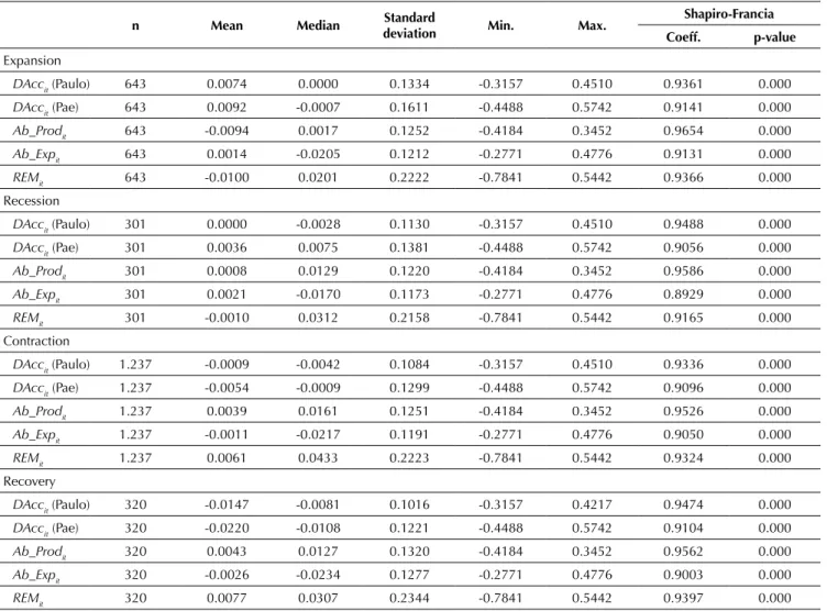
Table 2 presents the descriptive statistics of the earnings management proxies used in this study separated by phase of the business cycle.
Table 2
Descriptive statistics and normality test of the research variables covering 2000 to 2015
n Mean Median Standard
deviation Min. Max.
Shapiro-Francia Coeff. p-value
Expansion
DAccit(Paulo) 643 0.0074 0.0000 0.1334 -0.3157 0.4510 0.9361 0.000
DAccit(Pae) 643 0.0092 -0.0007 0.1611 -0.4488 0.5742 0.9141 0.000
Ab_Prodit 643 -0.0094 0.0017 0.1252 -0.4184 0.3452 0.9654 0.000
Ab_Expit 643 0.0014 -0.0205 0.1212 -0.2771 0.4776 0.9131 0.000
REMit 643 -0.0100 0.0201 0.2222 -0.7841 0.5442 0.9366 0.000
Recession
DAccit(Paulo) 301 0.0000 -0.0028 0.1130 -0.3157 0.4510 0.9488 0.000
DAccit(Pae) 301 0.0036 0.0075 0.1381 -0.4488 0.5742 0.9056 0.000
Ab_Prodit 301 0.0008 0.0129 0.1220 -0.4184 0.3452 0.9586 0.000
Ab_Expit 301 0.0021 -0.0170 0.1173 -0.2771 0.4776 0.8929 0.000
REMit 301 -0.0010 0.0312 0.2158 -0.7841 0.5442 0.9165 0.000
Contraction
DAccit(Paulo) 1.237 -0.0009 -0.0042 0.1084 -0.3157 0.4510 0.9336 0.000
DAccit(Pae) 1.237 -0.0054 -0.0009 0.1299 -0.4488 0.5742 0.9096 0.000
Ab_Prodit 1.237 0.0039 0.0161 0.1251 -0.4184 0.3452 0.9526 0.000
Ab_Expit 1.237 -0.0011 -0.0217 0.1191 -0.2771 0.4776 0.9050 0.000
REMit 1.237 0.0061 0.0433 0.2223 -0.7841 0.5442 0.9324 0.000
Recovery
DAccit(Paulo) 320 -0.0147 -0.0081 0.1016 -0.3157 0.4217 0.9474 0.000
DAccit(Pae) 320 -0.0220 -0.0108 0.1221 -0.4488 0.5742 0.9104 0.000
Ab_Prodit 320 0.0043 0.0127 0.1320 -0.4184 0.3452 0.9562 0.000
Ab_Expit 320 -0.0026 -0.0234 0.1277 -0.2771 0.4776 0.9003 0.000
REMit 320 0.0077 0.0307 0.2344 -0.7841 0.5442 0.9397 0.000
Note: the variables are described in the text. Source: Elaborated by the authors.
𝐷𝐷𝐷𝐷𝐷𝐷𝐷𝐷��= 𝛼𝛼 + 𝛽𝛽��𝐶𝐶𝐶𝐶𝐷𝐷𝐶𝐶𝐶𝐶��+ 𝛽𝛽��𝑈𝑈𝑈𝑈𝐶𝐶𝑈𝑈𝑈𝑈_𝑅𝑅𝑅𝑅𝑅𝑅��+ 𝛽𝛽��∆𝐺𝐺𝐷𝐷𝐺𝐺��+ 𝛽𝛽��𝑆𝑆𝑆𝑆𝑆𝑆𝐶𝐶��+ 𝛽𝛽��𝑅𝑅𝑅𝑅𝐷𝐷��
1
+𝛽𝛽��𝐿𝐿𝐶𝐶𝐿𝐿��+ 𝛽𝛽��𝐼𝐼𝐼𝐼𝑅𝑅𝑆𝑆�+ 𝜀𝜀��
2 3
The DAccit variable, estimated by both the Pae (2005) model and by the Paulo (2007) model, presented, on average, similar signs in all four phases of the business cycles, with positive signs in the expansion and recession phases, indicating a greater amount of positive accruals. In contrast, the negative signs in the contraction and recovery phases indicate, on average, a greater amount of negative values. That is, there are indications that managers manage their earnings upwards in the expansion and economic recession phases and manage them downwards during contractions and recoveries, using accruals.
The proxy for operational decisions, REMit, presented,
on average, opposing signs to those found for DAccit,
in this case negative for the expansion and recession
phases, indicating lower levels of REMit in these phases.
The positive signs for contraction and recovery indicate a greater use of this strategy by managers in these phases.
The opposing signs between DAccit andREMit between the
phases may indicate a trade-off in the choice of strategy used by managers, depending on the phase of the business cycle. In the other phases, the signs are the opposite of
Ab_Expit and Ab_Prodit, indicating, on average, that both
strategies act in favor of the REMit sign.
Table 3 presents the Spearman (non-parametric) correlation and Pearson (parametric) correlation matrix of the variables used in the regressions that respond to the problems of the study. However, as the Shapiro-Francia normality test (Table 2) indicates that all the variables do not present a normal distribution, for analysis purposes the use of the Spearman non-parametric correlation is recommended (Levin & Fox, 2004).
From the analysis of the correlation between the variables in the study, a strong correlation (> 0.7) stands
out between DAccit, estimated by the Pae (2005) and
Paulo (2007) models, as was already expected, since both concern discretionary accruals estimated by different models. However, the relationship between these and
REMit is positive for the Paulo (2007) model and negative
in relation to the other model. The explanation lies in the fact that the Paulo (2007) model already controls, in
the estimation of the residuals, the effect of REM on the
firms’ total accruals. The Ab_Prodit and Ab_Expit variables
also presented a strong correlation with REMit, given that
both are used for calculating this proxy.
Table 3
Spearman (lower part of the triangle) and Pearson (upper part of the triangle) correlation matrix
DAccit
(Paulo)
DAccit
(Pae)
Ab_
Prodit Ab_Expit REMit Sizeit ROAit Levit IFRSt ∆%GDPit EXPit RECESit CONTit RECOVit
DAccit (Paulo) 1 0.840 0.009 -0.014 0.006 -0.008 0.016 0.029 -0.022 0.048 0.040 0.001 -0.004 -0.048
DAccit(Pae) 0.7647 1 -0.112 0.045 -0.091 0.086 0.224 -0.068 -0.022 0.057 0.050 0.017 -0.019 -0.053
Ab_Prodit 0.0307 -0.0971 1 -0.666 0.912 -0.007 -0.308 0.119 0.080 -0.045 -0.045 0.002 0.029 0.013
Ab_Expit -0.0352 0.0321 -0.6057 1 -0.906 -0.050 -0.045 -0.110 -0.052 0.026 0.008 0.007 -0.007 -0.007
REMit 0.0318 -0.0766 0.8930 -0.8672 1 0.023 -0.142 0.128 0.073 -0.043 -0.030 -0.004 0.021 0.011
Sizeit 0.0013 0.0933 -0.0221 -0.0589 0.0065 1 0.309 0.019 0.173 -0.069 -0.089 0.000 0.067 0.016
ROAit -0.0180 0.2007 -0.4128 0.0224 -0.2468 0.1967 1 -0.405 -0.078 0.122 0.046 0.054 -0.086 0.016
Levit 0.0468 -0.0420 0.1139 -0.1176 0.1165 0.2435 -0.2553 1 0.049 -0.074 -0.043 -0.026 0.059 -0.008
IFRSt -0.0355 -0.0209 0.1083 -0.0782 0.1058 0.1775 -0.1152 0.0650 1 -0.407 -0.595 0.105 0.388 0.096
∆%GDPit 0.0326 0.0495 -0.0475 0.0218 -0.0420 -0.0456 0.1408 -0.0652 -0.3202 1 0.538 0.390 -0.732 0.012
EXPit 0.0284 0.0327 -0.0576 0.0213 -0.0466 -0.0913 0.0645 -0.0515 -0.5951 0.5677 1 -0.218 -0.582 -0.225
RECESit 0.0088 0.0379 -0.0045 0.0143 -0.0090 -0.0002 0.0728 -0.0237 0.1051 0.4915 -0.2176 1 -0.366 -0.142
CONTit -0.0068 -0.0174 0.0430 -0.0190 0.0389 0.0682 -0.1071 0.0639 0.3876 -0.8137 -0.5820 -0.3659 1 -0.379
RECOVit -0.0357 -0.0536 0.0153 -0.0135 0.0114 0.0176 0.0049 -0.0051 0.0961 -0.0037 -0.2253 -0.1417 -0.3789 1
Note: the variables are described in the text. Source: Elaborated by the authors.
From the control variables included in the models and considering the Spearman correlation, it can be
noted that only Levit and IFRSt were significant for the
Paulo (2007) model. In relation to the Pae (2005) model,
besides leverage, Sizeit and ROAit were also significant.
Regarding real earnings management, ROAit, Levit, and
IFRSt were significant. Thus, it is expected that adding
these variables to the models can control the effect on earnings management by these firm characteristics.
estimated by the models. The expansion and recession phases have a significant positive correlation with the discretionary accruals based on the Pae (2005) model.
The expansion and contraction phases of business cycles were also significant for REM.
Figure 3 Behavior of the earnings management proxies between 2000 and 2015
AEM = accruals-based earnings management; REM = real earnings management; GDP = gross domestic product. Source: Elaborated by the authors.
Figure 3 describes the behavior of the EM proxies and the GDP of Brazil for the analysis period. In order to improve its visualization, only the discretionary accruals obtained in accordance with the Paulo (2007) model were used, given that this presented a strong correlation with what was obtained by the Pae (2005) model. From Figure 3, it is perceived that both strategies (AEM and REM) move together from 2000 until 2005, when an inverse relationship between the two EM strategies begins. These two strategies present a positive relationship again at the end of 2012 until 2013, when the relationship between the levels of earnings management inverts once more. This last phase occurs precisely when the Brazilian economy begins to cool down, with consecutive periods of negative GDP growth below the average for the analysis, a period which, in accordance with Schumpeter (1939), is classified as a contraction. However, these observations are only based on the graphic analysis and only considered the variations in GDP, the basis for the classification of the phases of business cycles, which are the focus of this study. Thus, more robust analyses are presented in the next sections.
4.2. Analysis of Earnings Management in the Phases of Business Cycles
In order to verify the significance of the variables referring to the phases of business cycles in relation to AEM and REM, an unbalanced panel data analysis was
carried out. Initially, an analysis was conducted of which model most adapted to the data: random effects, fixed effects, or pooled ordinary least squares (POLS). For all the regressions used to estimate the abnormal behavior of the variables related with EM, the Breusch-Pagan tests were used, which verify the adequacy of the POLS model in relation to the random effects model; in this case, the results indicated that the POLS model is not the most adequate. The Hausman test verifies whether the random effects model provides more consistent estimates of the parameters in relation to the fixed effects models, and the results also rejected the null hypothesis; that is, the random effects model does not adapt better to the data in relation to the fixed effects panel. Finally, the Chow tests also rejected the null hypothesis, confirming that the fixed effects model fits the data. This procedure was carried out for all the equations and the results were identical. The statistical tests of the models indicate that all reject the null hypothesis of normality by means of the Jarque-Bera test. However, in accordance with the central limit theorem, Wooldridge (2014) claims that in large samples the presumption of normality can be relaxed. The Wald and Wooldridge tests also revealed the presence of heteroskedasticity and autocorrelation, respectively, in practically all the models. With the aim of correcting their effects in the regressions, the models were estimated with robust or clusterized standard errors, when this was the case.
-0.08 -0.06 -0.04 -0.02 0 0.02 0.04 0.06 0.08
2000 2002 2004 2006 2008 2010 2012 2014
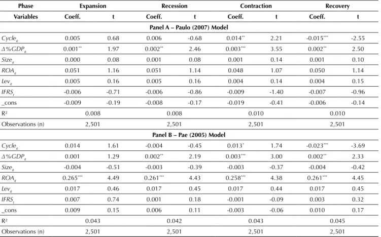
Table 4 presents the results of the regressions concerning the relationship between the economic environment and AEM by the Pae (2005) and Paulo (2007) models.
Table 4
Relationship between the business cycles and AEM – 2000 to 2015
Phase Expansion Recession Contraction Recovery
Variables Coeff. t Coeff. t Coeff. t Coeff. t
Panel A – Paulo (2007) Model
Cycleit 0.005 0.68 0.006 -0.68 0.014** 2.21 -0.015*** -2.55
∆%GDPit 0.001** 1.97 0.002** 2.46 0.003*** 3.55 0.002** 2.50
Sizeit 0.000 0.08 0.001 0.08 0.001 0.14 0.001 0.10
ROAit 0.051 1.16 0.051 1.14 0.048 1.07 0.050 1.14
Levit 0.005 0.16 0.005 0.16 0.004 0.14 0.004 0.15
IFRSt -0.006 -0.71 -0.006 -0.86 -0.009 -1.40 -0.007 -0.96
_cons -0.009 -0.19 -0.008 -0.17 -0.019 -0.41 -0.006 -0.14
R² 0.008 0.008 0.010 0.010
Observations (n) 2,501 2,501 2,501 2,501
Panel B – Pae (2005) Model
Cycleit 0.014 1.61 -0.004 -0.45 0.013* 1.74 -0.023*** -3.69
∆%GDPit 0.001 1.29 0.002** 2.19 0.003*** 3.00 0.002** 2.33
Sizeit -0.004 -0.51 -0.003 -0.39 -0.003 -0.37 -0.004 -0.42
ROAit 0.265
*** 4.49 0.261*** 4.43 0.258*** 4.38 0.261*** 4.45
Levit 0.017 0.46 0.017 0.45 0.017 0.44 0.017 0.45
IFRSt 0.007 0.74 0.001 0.18 -0.001 -0.09 0.003 0.32
_cons 0.009 0.15 0.006 0.11 -0.003 -0.06 0.010 0.17
R² 0.043 0.042 0.043 0.045
Observations (n) 2,501 2,501 2,501 2,501
Note: the variables are described in the text. AEM = accruals-based earnings management.
*, **, *** = significant to the level of 1%, 5%, and 10%, respectively. Source: Elaborated by the authors.
In general, the results of Table 4 show a low explanatory power of the variations in the accruals estimated by both models, and only some variables of the models were presented as significant.
Regarding the relationship between EM and the phases of the business cycles, it is verified that during the contraction phase companies engage in earnings management, increasing the level of discretionary
accruals, since the Cycleit variable presented a positive
sign that was statistically significant to 10% and to 5% in this phase, according to the Pae (2005) and Paulo (2007) models, respectively. In this phase, the economy presents consecutive negative variations in GDP, including below the mean; that is, in this period of considerable economic slowdown, firms increase their level of accruals-based
earnings management. The coefficients of the CONTit
(contraction) variable for the Pae (2005) and Paulo (2007)
models were 0.013 and 0.014, respectively, indicating that a positive variation occurred in the discretionary accruals in this phase, on average 1.3% and 1.4% greater than in relation to the other phases.
In the recovery period, there are indications that managers reduce the level of discretionary accruals,
since the Cycleit variable was negative and significant for
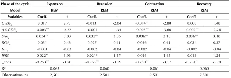
Table 5 presents the results of the relationship between REM and the economic environment.
Table 5
Relationship between the business cycles and REM – 2000 to 2015
Phase of the cycle Expansion Recession Contraction Recovery
Model REM REM REM REM
Variables Coeff. t Coeff. t Coeff. t Coeff. t
Cycleit 0.017 2.73 -0.013** -2.04 -0.014*** -2.88 0.008 1.48
∆%GDPit -0.003*** -2.77 -0.001 -1.34 -0.003*** -3.60 -0.002*** -2.26
Sizeit 0.034*** 3.00 0.035*** 3.06 0.036*** 3.18 0.036*** 3.18
ROAit 0.031 0.48 0.027 0.41 0.026 0.41 0.024 0.37
Levit -0.001 -0.03 -0.002 -0.04 -0.002 -0.04 -0.002 -0.04
IFRSt 0.022** 1.96 0.021* 1.57 0.016 1.45 0.013 1.24
_cons -0.253*** -3.20 -0.253*** -3.19 -0.250*** -3.17 -0.261*** -3.29
R² 0.062 0.060 0.061 0.060
Observations (n) 2,501 2,501 2,501 2,501
Note: the variables are described in the text. REM = real earnings management.
*, **, *** = significant to the level of 1%, 5%, and 10%, respectively. Source: Elaborated by the authors.
The results in Table 5 reveal the significant and negative relationship between both the recession and contraction
phases and REMit, indicating a reduction in the level of
this earnings management strategy, precisely in this phase in which the economy presents a negative variation in GDP growth, after a period of consecutive rises. That is, managers appear to adjust firm operations to cope with this period of slowdown in the economy. For the recession
phase, the RECESit variable in the estimation for the real
earnings management model has a negative coefficient of 0.013, indicating that abnormal behavior in the firms’ operational activities undergoes a negative variation, by an average of 1.3% in relation to the other phases of the
business cycle, while in the contraction (CONTit) phase,
the abnormal behavior of real activities undergoes an average reduction of 1.4%.
Including the GDP variation in the earnings management models serves to capture the fluctuations in the economy so that the proxies for AEM and REM only reflect the discretionary behavior of managers in manipulating accounting earnings (Cohen & Zarowin,
2007). In Table 4, it is observed that the Δ%GDPit variable
was positive and significant in all the estimates, except in the expansion phase for AEM measured by the Pae (2005) model and in recession for the abnormal behavior of operational activities (Table 5).
These results indicate that the discretionary accruals and the abnormal behavior of real activities are related with the phases of the business cycle, therefore it is important to control the effects of the cycles in studies
on accruals-based and/or real earnings management. In addition, for the sample of this study, the results suggest an average variation in discretionary accruals of between 0.1% and 0.3% for every 1 percentage point variation in GDP, depending on the phase of the business cycle. For example, in contraction, if there was 1% increase in GDP, accruals would increase by 0.3%. Note that this finding suggests that part of the variation in the abnormal behavior of accruals is related with the business cycle and not with the discretionary behavior of managers.
Regarding real earnings management, the variation in GDP, which is a proxy for the performance of economic activities, also influences the volume of real activities, with
the results indicating that the Δ%GDP explainsbetween
0.1% and 0.3% of the variation in the abnormal behavior of the real activities of the firms in the sample. That is, as expected, the firms’ (real) operational activities are influenced by macroeconomic factors. Thus, as observed in the behavior of the accruals, a portion of the variation in the firms’ operational activities is also related to the macroeconomic environment, and not only to the opportunistic behavior of managers.
4.3. Analysis of the Trade-Off between the Earnings Management Strategies in the Phases of the Business Cycles
Preliminarily, the volumes of the residuals of the accruals estimation model were compared with the residuals of the operational activities estimation models.
In Table 6, it is observed that the AEMit variable has a
positive sign in the expansion and recession phases,
while the REMit variable has a negative sign in these
phases. However, there is an inversion of signs between
the AEMit and REMit variables in the contraction and
recovery phases. This may suggest a trade-off between the two EM strategies.
Table 6
Comparison between the average for AEM and REM – 2000 to 2015
Phase of the cycle Expansion Recession Contraction Recovery
Model Mean Standard
deviation Mean
Standard
deviation Mean
Standard
deviation Mean
Standard deviation
AEM Paulo 0.0074 0.1334 0.0000 0.1113 -0.0009 0.1084 -0.0147 0.1016
Pae 0.0092 0.1611 0.0036 0.1381 -0.0054 0.1299 -0.0220 0.1221
REM -0.0100 0.2222 -0.010 0.2158 0.0061 0.2223 0.0077 0.2344
AEM = accruals-based earnings management; REM = real earnings management. Source: Elaborated by the authors.
In addition, an inversion of the signs is also observed
for the estimations of the coefficients of the Cycleit variable
between the AEMit (Table 4) and REMit (Table 5) models or
a loss of statistical significance, as summarized in Table 7. These results may also suggest the confirmation of a trade-off between accruals-based and real earnings management.
Table 7
Comparison between the coefficients of the model for AEM and REM – 2000 to 2015
Phase of the cycle Expansion Recession Contraction Recovery
Model Coeff. t Coeff. t Coeff. t Coeff. t
AEMit Paulo 0.005 0.68 0.006 -0.68 0.014
** 2.21 -0.015*** -2.55
Pae 0.014 1.61 -0.004 -0.45 0.013* 1.74 -0.023*** -3.69
REMit 0.017 2.73 -0.013** -2.04 -0.014*** -2.88 0.008 1.48
AEM = accruals-based earnings management; REM = real earnings management. *, **, *** = significant to the level of 1%, 5%, and 10%, respectively.
Source: Elaborated by the authors.
The results also indicated a reduction in REM in the period of the recession and contraction. The use of accruals in the phases in which the economy is presenting positive variations and the reduction in the level of REM when it begins to present negative variations could be explained because REM is considered more expensive than AEM, since REM directly impacts the firm’s cash flow (Cohen & Zarowin, 2007; Zang, 2012). That is, in
the expansion and recovery phases, periods of GDP growth, managers prefer not to engage in this type of management and also reduce the level when the economy slows down.
For greater robustness in the analysis of hypothesis 2 of this study, Table 8 presents the estimations for the model (Equation 11) that seeks to capture the trade-off between the AEM and REM earnings management strategies.
Table 8
Analysis of the trade-off between AEM and REM in the business cycles – 2000 to 2015 Panel A – Paulo (2007) Model
Phase of the cycle Expansion Recession Contraction Recovery
Variables Coeff. t Coeff. t Coeff. t Coeff. t
Cycleit 0.006 0.72 -0.006 -0.75 0.014** 2.22 -0.015*** -2.51
Unexp_REMit -0.054* -1.72 -0.054* -1.71 0.051* -1.63 -0.052* -1.65
∆%GDPit 0.001* 1.84 0.002** 2.40 0.003*** 3.50 0.002** 2.40
Panel A – Paulo (2007) Model
Phase of the cycle Expansion Recession Contraction Recovery
Variables Coeff. t Coeff. t Coeff. t Coeff. t
ROAit 0.063 1.42 0.062 1.40 0.059 1.32 0.061 1.39
Levit 0.001 0.03 0.001 0.03 0.006 0.02 0.009 0.03
IFRSt -0.006 -0.73 -0.007 -0.88 -0.010 -1.44 -0.007 -1.01
_cons -0.018 -0.39 -0.017 -0.37 -0.028 -0.61 -0.016 -0.35
R² 0.011 0.011 0.012 0.013
Observations (n) 2,501 2,501 2,501 2,501
Panel B – Pae (2005) Model
Cycleit 0.014 1.67 -0.005 -0.55 0.013* 1.76 -0.023*** -3.58
Unexp_REMit -0.093** -2.40 -0.091** -2.35 -0.089** -2.29 -0.089** -2.29
∆%GDPit 0.001 1.06 0.002** 2.07 0.003*** 2.89 0.002** 2.14
Sizeit -0.002 -0.20 -0.001 -0.09 -0.001 -0.06 -0.001 -0.11
ROAit 0.285*** 4.94 0.280*** 4.86 0.277*** 4.80 0.280*** 4.88
Levit 0.011 0.30 0.011 0.29 0.010 0.28 0.011 0.29
IFRSt 0.007 0.66 0.001 0.12 -0.002 -0.19 0.002 0.21
_cons -0.008 -0.13 0.010 -0.17 -0.020 -0.33 -0.007 0.11
R² 0.049 0.047 0.048 0.051
Observations (n) 2,501 2,501 2,501 2,501
Note: the variables are described in the text.
AEM = accruals-based earnings management; REM = real earnings management. *, **, *** = significant to the level of 1%, 5%, and 10%, respectively.
Source: Elaborated by the authors.
Comparatively analyzing the estimations of the discretionary accruals in the four phases of the business cycle, it is verified that there were no significant differences in the coefficients with or without the REM control (tables 4 and 5, respectively). Only the R² of the models obtained a small average rise of 0.05 for the Pae (2005) model and of 0.03 for the Paulo (2007) model.
Concerning the analysis of the trade-off between the EM
strategies, the coefficients of the Unexp_REMit variable were
negative and significant in all the phases of the business cycle, for both discretionary accruals estimations models (Pae, 2005; Paulo, 2007). These results suggest that there is a trade-off between accruals-based and real earnings management; thus, the second research hypothesis cannot be rejected.
5. FINAL REMARKS
This study aimed to verify the influence of the economic environment over earnings management strategies in Brazilian public companies. To achieve the objective of the research, the four phases of business cycles, based on Schumpeter (1939), were used as a proxy for the economic environment, in addition to the abnormal behavior of accruals and of operational activities for EM.
As the first research hypothesis, it was established that accruals-based earnings management is influenced by business cycles. The results found indicate that it was not possible to reject the hypothesis, as they revealed that managers increase the level of accruals in the contraction phase, that is, precisely at the time of economic slowdown, and they reduce them in recovery. By considering the level of firms’ accruals as one of the
measures of accounting information quality, the findings of this study are in line with the studies that have shown a deterioration in earnings quality in crisis periods (Iatridis & Dimitras, 2013; Persakis & Iatridis, 2015; Tahinakis, 2014; Trombetta & Imperatore, 2014), since Borio (2014) reports that financial crises are generally accompanied by the recession phase of the business cycle. However, in his study the author considered only two phases of the cycle, in accordance with the NBER classification. As this study divides the recession phase into two, recession and contraction, it cannot be claimed that the level of EM worsens in the recession phase.
The evidence also indicated that in the recession and contraction phases, that is, when the economy has slowed down after consecutive periods of positive GDP growth, managers reduce the level of real earnings management.
With regard to the trade-off between accruals-based and real earnings management, the results indicate an inverse relationship between these two discretionary practices. Thus, it was not possible to reject the second research hypothesis, which establishes that the business cycle has an impact on the choice of EM strategies.
Including the variable related to GDP fluctuations provided an improvement in the explanatory power of the models, as well as being significant in the analysis of the business cycles. In addition to indicating the influence of the economic environment on the firms’ accounting numbers, this process enabled the variables of the earnings management analysis to significantly represent managers’ discretionary actions. The results suggest that the abnormal behaviors of accruals and of real operational activities are related to the macroeconomic environment and not only to the opportunistic behavior of managers. This finding implies that the studies that analyze accruals-based and/ or real earnings management should control the variation in GDP to obtain more robust results.
The results found add new knowledge in relation to the behavior of EM in the face of fluctuations in
the economic, just like the studies in times of financial crises or those that have used the binary classification of business cycles.
This study differs from the rest by confirming the relationship between earnings management and the four phases of the business cycle, as well as by identifying the trade-off between the two earnings management strategies in relation to the economic environment. In addition, with regard to accounting information quality, which can change depending on the phase of the business cycle, the findings presented in this study could be used by investors and lenders in their decision making, such as in the allocation of resources in the capital and credit market; by regulators in the elaboration of rules and their possible pro-cyclical effects; and by the other users of accounting information in evaluating the performance of managers and companies.
The results of this study are limited to the period analyzed and, specifically, to the Brazilian stock market. Finally, we suggest verifying the reasons that lead managers to choosing some of the earnings management strategies in relation to the four phases of business cycles.
REFERENCES
Ardison, K. M. M., Martinez, A. L., & Galdi, F. C. (2012). The effect of leverage on earnings management in Brazil. ASAA - Advances in Scientific and Applied Accounting, 5(3), 305-324. Ball, R., & Brown, P. (1968). An empirical evaluation of
accounting income numbers. Journal of Accounting Research, 6(2), 159-178.
Barros, C. M. E., Soares, R. O., & Lima, G. A. S. de F. (2013). A relação entre governança corporativa e gerenciamento de resultados em empresas brasileiras. Revista de Contabilidade e Organizações, 7(19), 27-39.
Barros, M. E., Menezes, J. T., Colauto, R. D., & Teodoro, J. D. (2014). Gerenciamento de resultados e alavancagem financeira em empresas brasileiras de capital aberto. Contabilidade, Gestão e Governança, 17(1), 35-55. Beaver, W. (1968). The information content of earnings
announcements. Journal of Accounting Research, 6, 67-92. Bekiris, F. V., & Doukakis, L. C. (2011). Corporate governance
and accruals earnings management. Managerial and Decision Economics, 32(7), 439-456.
Borio, C. (2014). The financial cycle and macroeconomics: what have we learnt? Journal of Banking & Finance, 45(1), 182-198. Burns, A. F., & Mitchell, W. C. (1946). Measuring business cycles.
New York, NY: National Bureau of Economic Research. Claessens, S., Kose, M. A., & Terrones, M. E. (2012). How do
business and financial cycles interact? Journal of International Economics, 87(1), 178-190.
Cohen, D. A., & Zarowin, P. (2007). Earnings management over the business cycle. New York University/Stern School
of Business. Retrieved from http://web-docs. stern.nyu.edu/ old_web/emplibrary/EM_08_23_07FINAL.pdf.
Cohen, D. A., & Zarowin, P. (2010). Accrual-based and real earnings management activities around seasoned equity offerings. Journal of Accounting and Economics, 50(1), 2-19. Davis-Friday, P. Y., Eng, L. L., & Liu, C. S. (2006). The effects of
the Asian crisis, corporate governance and accounting system on the valuation of book value and earnings. The International Journal of Accounting, 41(1), 22-40.
Defond, M. L., & Jiambalvo, J. (1994). Debt covenant violation and manipulation of accruals. Journal of Accounting and Economics, 17, 145-176.
Dimitras, A. I., Kyriakou, M. I., & Iatridis, G. (2015). Financial crisis, GDP variation and earnings management in Europe. Research in International Business and Finance, 34(C), 338-354. Domingos, S. R. M., Ponte, V. M. R., Paulo, E., & Alencar, R. C.
de (2017). Gerenciamento de resultados contábeis em oferta pública de ações. Revista Contemporânea de Contabilidade, 14(31), 89-107.
Filip, A., & Raffournier, B. (2014). Financial crisis and earnings management: the European evidence. The International Journal of Accounting, 49(4), 455-478.
Grecco, M. C. (2013). O efeito da convergência brasileira às IFRS no gerenciamento de resultados das empresas abertas brasileiras não financeiras. BBR – Brazilian Business Review, 10(4), 117-140.