doi: 10.1590/0101-7438.2017.037.03.0487
SHORTEST PATHS ON DYNAMIC GRAPHS: A SURVEY
Daniele Ferone, Paola Festa
*, Antonio Napoletano and Tommaso Pastore
Received April 31, 2017 / Accepted October 23, 2017
ABSTRACT.This paper provides an overview of the state-of-the art and the current research trends con-cerning shortest paths problem on dynamic graphs. The discussion is divided in two main topics: reop-timization and time-dependent shortest paths. Reopreop-timization consists in the solution of a sequence of shortest path problems in which each instance slightly differs from the previous one. The reoptimization tackles this problem wisely using information stored in an optimal solution previously computed. On the other hand, shortest path problems on time-dependent graphs are characterized by a weight function which not only depends upon the arcs but changes in time according to a certain time horizon.
Keywords: Shortest Path, Network Optimization, Network Flows, Structure path constraints, Labelling methods, Auction Method.
1 INTRODUCTION
One of the most iconic algorithms in combinatorial optimization is due to Dijkstra [21], who in 1959 devised a label setting algorithm for theshortest path problem (SPP). Since then, the SPP established itself as one of the most representative problems of operations research. Indeed, even today, many combinatorial optimization problems (COPs) require the solution of SPP as sub-task. Some examples of these problems are Maximum-Flow Minimum-Cost Problems [2], Vehicle Routing Problems [64], and several other variations of the SPP, spanning from problems on time-dependent graphs [49, 50] to general constrained SPP [25, 57].
Reoptimizing shortest paths on dynamic graphs consists in solving a sequence of shortest path problems, where each problem differs only slightly from the previous one, because the origin node has been changed, some arcs have been removed from the graph, or the cost of a subset of arcs has been modified. Each problem could be simply solved from scratch, independently from the previous one, by using either alabel-correctingor a label-settingshortest path algorithm. Nevertheless, a clever way to approach it is to design ad hoc algorithms that efficiently use information resulting from previous computations.
*Corresponding author.
Department of Mathematics and Applications “R. Caccioppoli”, University of Napoli Federico II, Italy.
Another type of dynamic graph is thetime-dependent graph, introduced in Cooke & Halsey [13], where the characteristic cost functionwis defined for each edge(i, j), aswi j(t), wheret is a
time variable in a time domainT. The valuewi j(t)specifies how much time it takes to travel from
nodei to node j, if departing fromi at the timet. Most of the solution strategies for problems on dynamic graphs (often called networks) have been adopted to solve instances of shortest path problems on time-dependent graphs.
In the wholeness of its variations, shortest path problems on dynamic graphs appear in a wide variety of contexts and application settings, including logistics, telecommunications, transporta-tion, urban traffic, and transit planning.
The remainder of the paper is organized as follows. In Section 2 the shortest path problems are formally introduced and the classical approaches to solve them are presented. Sections 3 and 4 analyze the scientific literature of reoptimization and time-dependent graphs, respectively. Conclusions and final remarks are given in Section 5.
2 MATHEMATICAL FORMULATIONS AND CLASSICAL APPROACHES
2.1 Mathematical Formulation of the Shortest Paths Problem
In this section, the mathematical formulation for all types of shortest path problems is given. Indeed, SPPs can be classified in three different sub-categories: shortest path point-to-point (P2P), shortest path tree (SPT), and all pairs shortest paths (APSP).
All these problems rely on the following notation. LetG=(V,A)be a directed weighted graph, where:
• V = {1,2, . . . ,n}is a set of nodes;
• A⊆ {(i,j)∈V ×Vi,j ∈V ∧i= j}is a set ofmarcs;
• w: A→R+is a function that assigns a non-negative costwi jto each arc(i,j)∈ A.
Furthermore, for eachi =1, . . . ,n, let
• F S(i)= {j ∈V(i,j)∈ A}be theforward starof nodei;
• B S(i)= {j ∈V(j,i)∈ A}be thebackward starof nodei.
2.2 Shortest path point-to-point problem (P2P)
The problem consists in finding a shortest pathP∗=(v1, v2, . . . , vh)from a source nodev1=s to a destination nodevh = t, withs,t ∈ V. Introducingm Boolean decision variables, xi j,
∀(i,j)∈ A, such that:
xi j =
1, if(i,j)belongs toP∗,
the mathematical formulation of the (P2P) problem is the following:
(P2P) z=min
(i,j)∈A
wi jxi j
subject to:
(P2P-1)
j∈B S(i)
xj i −
j∈F S(i)
xi j =bi, ∀i∈V
(P2P-2) xi j ∈ {0,1}, ∀(i,j)∈ A,
withbi = −1 for i=s, bi =1 for i=t, and bi =0 otherwise.
2.3 Shortest path tree problem (SPT)
Given a noder ∈ V, namedroot, the goal of the problem is to find a shortest path fromr to all other nodesi ∈ V, i = r. Definingm Boolean decision variables xi j,∀ (i,j) ∈ A, the mathematical formulation of the (SPT) problem is the following:
(SPT) z=min
(i,j)∈A
wi jxi j
subject to:
(SPT-1)
j∈B S(i)
xj i −
j∈F S(i)
xi j =bi, ∀i ∈V;
(SPT-2) xi j ≥0, ∀(i,j)∈ A.
where bi = −n+1 for i=r, and,bi =1 for i =r.
2.4 All pairs shortest path problem (APSP)
The aim of this problem is to find all the point-to-point shortest paths between each pair of nodes i, j ∈ V, i = j. Its mathematical formulation can be easily obtained starting from the mathematical formulation of the SPT. With few modifications, the following model can be obtained:
(APSP) z=min
n
k=1
(i,j)∈A
wi jxi jk
subject to:
(APSP-1)
j∈B S(i)
xkj i− j∈F S(i)
xi jk =bik, ∀i ∈V,∀k∈V;
(APSP-2) xi jk ≥0, ∀(i,j)∈ A, ∀k∈V,
2.5 Labeling Methods
A first successful attempt to solve the SPP was originally proposed by Ford Jr [28] and Ford Jr & Fulkerson [29], although the most famous algorithm to solve P2P and SPT is a labeling method proposed by Dijkstra [21], whose pseudo-code is reported in Figure 1. Lets ∈V be the source node in a graphG, to find a shortest path fromsto each otherv∈V,i =s, Dijkstra’s algorithm maintains and updates for each nodev∈V:
• dist[v], the distance ofvfrom the source nodes;
• pred[v], the predecessor of the nodevin the incumbent path fromstov.
In addition, the following sets are used: SandQ, that are the sets of visited and unvisited nodes, respectively.
The algorithm starts with an initialization phase (lines 2-5), where the vectorspred,distand the sets S andQare initialized. Afterwards, while set Qis nonempty, the algorithm selects an unvisited nodev, relaxes all the edges inF S(v), and insertvinS. The relaxation operation is described in lines 10-12.
If the weight functionwis non-negative, the algorithm always terminates with the correct shortest path distances stored indist[], and shortest path tree inpred[]. The following theorem holds:
Theorem 1. If the cost functionw is non-negative, then Dijkstra’s algorithm visits nodes in non-decreasing order of their distances from the source, and visits each node at most once.
Algorithm 1– Dijkstra’s algorithm 1: procedureDIJKSTRA(G=(V,A),s)
2: dist[s]:= 0;pred[s]:= NULL;S:=∅; 3: for allv∈V \ {s}do
4: dist[v]:=+∞;pred[v]:= NULL;
5: Q←V
6: whileQ= ∅do 7: u := extract min(Q);
8: S:=S∪ {u}; 9: for allv∈ F S(u)do
10: ifdist[v]>dist[u]+wuvthen
11: dist[v]:=dist[u]+wuv;
12: pred[v]:=u;
directions: the first from nodestot, called theforward search, and the latter fromt tos, the
backward search. The backward search operates on thereverse graph, obtained fromGreversing the direction of each arc inA. The algorithm terminates when the two paths meet.
Hart et al. [36] proposed another labeling method for SPP: an informed search algorithm called
A∗. It refines the Dijkstra’s method, using a best first paradigm, firstly exploring sub-paths which appear to lead most quickly to the solution.
The estimation of the most promising sub-paths is carried out by means of a potential function πt. Letπt :V →R+be a non-negative function, giving an estimate on the distance from each
nodev tot. The A∗ search uses a new setL, which contains all the nodes that are relaxed at least once and whose label is not permanent. It selects a nodev ∈ L with the smallest value of
k(v)=d(s, v)+πt(v), whered(s, v)is the shortest distance fromstov.
A potential functionπt is defined to befeasibleifdπ(u, v) =d(u, v)−πt(u)+πt(v)is
non-negative for each arc(u, v) ∈ A. Goldberg & Harrelson [34] showed that A∗ search with a feasible non-negative potential function visits no more nodes than Dijkstra’s algorithm.
In order to define πt, in the Euclidean domain, it is possible to use the canonical Euclidean
distance to establish a lower bound. Such computation is carried out by means of a method based on the concept of landmarks selection [34] and the triangle inequality.
3 REOPTIMIZATION
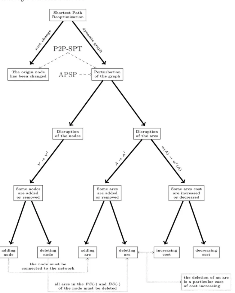
Nowadays, in the era of big data and huge networks, there is a rising need of well performing algorithms, able to handle the massive amount of available information. One of the suitable approaches to tackle this complexity is to reuse information already computed, in order to reduce the computational time needed to obtain an optimal solution. In the context of SPP, previous information can be reused while tackling a problem which differs only slightly from another SPP previously solved. This occurrence can happen with one of the following changes in the network:
• the origin node has been changed;
• some nodes have been added or removed;
• some arcs have been added or removed;
• some arcs weight have been increased or decreased.
This problem can be addressed as a shortest path reoptimization problem [26], which consists in solving a sequence of shortest path problems, where thekt hproblem marginally differs from the (k−1)t hone.
In the first case, we say that there was a root change from the(k −1)t h problem to thekt h
occur on the network. A dynamic graph is said to be fully dynamic if both insertion and deletion of either edges or nodes are allowed.
Figure 1–Reoptimization problems hierarchy.
node are addition or removal. On the other hand, the arcs can be either added/removed or their cost can be increased/decreased. It is worthy to note that the case of changes involving nodes implies also arcs insertion or deletion.
Without loss of generality, we can consider the input graphG = (V,A)as a complete graph. Indeed, ifGis not complete, for each pair of nodesiandj, such that(i,j)∈A, it can be always added a dummy arc fromito jwithwi j = +∞.
This operation allows the following considerations:
• arc removal in the graph can be seen as a special case of arc cost increasing. If an arc(i,j) is deleted, then the costwi j increases to+∞.
• Arc insertion can be seen as a special case of arc cost decreasing. If an arc(i,j), must be inserted, then the costwi jis decreased from+∞to the new costk.
3.1 Root change
The purpose of this paragraph is to show how, in the case of root change for the SPT problem, it is possible to obtain a well performing algorithm making wise use of the information stored in a SPT previously computed. Such result relies on some remarkable theoretical properties proven by Gallo [32], starting from the assumption that a single root shortest path tree problem has been solved.
LetG=(V,A)be a complete directed graph, and letTr be a shortest path tree rooted at noder,
i.e., a tree that contains a shortest path fromrto each nodev∈V, v=r. Letsbe a node ofV,
s=r, andTsbe a SPT rooted at nodes.
The following propositions show how the knowledge ofTr provides useful informations onTs.
LetTr(h)denote the subtree ofTr which contains nodehtogether with all its descendants, then
Proposition 1.Tr(s)⊆Ts and d(s,j)=d(r,j)−d(r,s), for any j ∈Tr(s).
Henceforth, the paths contained in the subtree ofTrrooted insstill remain optimal shortest paths fromsto its descendants. This result shows how a wise handling of the old solution is likely to be the most efficient strategy, since – especially when the new rootsis close tor– a consistent part of the previously optimal treeTr will remain optimal.
As formerly stated, beyond the theoretical insight given by Proposition 1, the information pro-vided byTr can be employed in order to reduce the computational time needed to solve the new
Letπ1, π2, . . . , πnbe integer numbers such that
li j =wi j +πi−πj ≥0 ∀(i,j)∈ A. (1)
Proposition 2. The problem of finding the SPT from s with arc lengthswi j is equivalent to the problem of finding the SPT with arc lengths li j given by(1).
Proof. Let P be a generic path from a nodekto a nodeh ofG =(V,A), and letW(P)and
L(P)be the lengths ofPpertaining to the length functionswandl, respectively. Then, it holds that
L(P)=
(i,j)∈P
li j =
(i,j)∈P
(wi j+πi −πj)=W(P)+(πk−πh). (2)
Henceforth, the lengthsW(P)andL(P)only differ by a constant depending only on the source and the destination nodes of the path.
Ultimately, a shortest path treeTr with respect to the arc lengthwi jwill remain optimal with arc
lengthli j.
A straightforward consequence of Proposition 2 is that lengthswi j can be replaced by lengths li j, and once the new shortest lengthd′(s,h),h ∈V, is found, the valued(s,h)can be obtained
as follows:
d(s,h)=d′(s,h)−πs+πh. (3)
The results outlined above suggest that an appropriate choice of the integersπi might decrease
the distance from the source to the farthest node, and thus also the computation time required by DDA. Indeed, when selectingπj =d(s, j)one hasd′(s,j)=0, for all j ∈ V, thus obtaining
the validity of the following proposition:
Proposition 3. Let beπj =d(r,j), for all j ∈ Tr, and let be the arc lengths defined as in(1). Let h be one of the farthest node from the origin s, then:
d′(s,h)=d(r,s)+d(s,r). (4)
From Proposition 3 it follows that if nodesr ands are close enough, the computational effort required by DDA can be strongly reduced by a cost modification of type (1), with the vectorπ given byπj =d(r,j), for all j∈Tr.
As reported in Gallo [32], in terms of Linear Programming, such new costs correspond to the reduced costs relative to a dual feasible, but primal unfeasible, basis. This interpretation of the vector(π1, π2, . . . , πn)as a dual feasible solution for the Shortest Path Problem is due to Bazaraa
& Langley [6].
techniques. This algorithm refines the classical label setting paradigm by partitioning the nodes of the graph in three distinct sets: N T,N P, and N Q. As in a classical label setting algorithm,
N T andN Pare the set of nodes whose labels are temporary and permanent, respectively. While, the nodes inN Q are those nodes such thatd(s, v)=d(s,p(v)). This property ensures that such nodes can be inserted straightaway inN Pwithout further comparisons, thus speeding up the ex-ecution of the algorithm. In [33], it has been noted how in any reoptimization problem instances a large share of nodes ofV is likely to be found inN Q.
The observations made by Gallo are the starting point of the work of Florian et al. [27]: the shortest path tree rooted at noderis an optimal solution to a corresponding linear program, but when a successive new sourcesis considered, the previous tree is a dual feasible and primal infeasible solution for the new problem. The approach proposed by Florian et al. [27] consists in the adaptation of the dual simplex method to compute the shortest paths from the new roots. It is shown in Florian et al. [27] that the proposed algorithm runs at most inO(n2).
In order to evaluate the performances of their method, the authors tested their code on graphs representing the regional roads of the cities of Vancouver and Winnipeg, as in Gallo [32].
The experimental evaluations proposed in these works show how Gallo [32] is slightly better performing than Dijkstra’s from scratch technique, meanwhile Gallo & Pallottino [33] further improves the previous results. Although, among all, the algorithm proposed by Florian et al. [27] appears to outperform the other competitive methods.
In Ferone et al. [26], a novel dual approach based on an auction framework [8] is presented. Given a shortest paths treeTr, and a new sources, all the arcs inB S(s)are deleted and the nodes of the treeTr(s)are included in a priority queueQ, containing the nodes ordered according to the
reduced costs in decreasing order.Qis analyzed with a strongly polynomial auction algorithm [10]. During the extraction of the nodes fromQ, when the algorithm reaches a node j ∈ Tr, it moves the sub-treeTr(j)fromTr toTs, and its nodes are included inQ. The algorithm terminates
whenQbecomes empty.
3.2 Arc Cost Change
Given a shortest paths tree,Tr, the problem of arc cost change consists in recalculating treeTr
when a new weight is assigned to one or more (batch updates) arcs. As extensively discussed in Gallo [32], the results of Theorem 4 can be used to derive algorithms that reoptimize the solution of a SPP after a change of the cost of a single arc.
Theorem 4 (Gallo [32]).Let Tr be a shortest paths tree,wu′vbe the new cost of the arc(u, v)∈
A, and S(u)= {v ∈ Vd(r, v) ≤ d(r,u)}. Denoting with Tr′ the new shortest paths tree, the following properties hold:
Tr(v)⊆Tr′(v),
j ∈Tr(v)⇒d′(r,j)=d(r,j)−wuv−wu′v
,
j ∈S(u)⇒d′(r,j)=d(r,j);
(ii) ifw′uv< wuvand(u, v) /∈Tr, then
Tr(v)⊆Tr′(v),
j ∈S(u)⇒d′(r,j)=d(r,j);
(iii) ifw′uv> wuvand(u, v)∈Tr, then
j ∈/ S(u)⇒d′(r,j)=d(r,j);
(iv) ifw′uv> wuvand(u, v) /∈Tr, then
Tr(v)=Tr′(v),
d′(r, j)=d(r,j) ∀j ∈V .
In other words, a decrease in the cost of the arc(u, v)(cases (i) and (ii)) implies that the sub-tree
Tr(v)remains part of the optimal solution and the optimal distances of its nodes accordingly decreased where necessary. Case (iii) tackles the cost increase when(u, v)is part of the solution, stating that the optimal distances are preserved for each j ∈S(u). Finally, in case (iv) the entire solution remains optimal.
Pallottino & Scutell`a [55] assume that a shortest paths treeTr has been determined and address the problem of computing the shortest paths tree when new costs are given to a subset K of the arcs ofG, either lower or higher than the old ones. The reoptimization framework used is based on the determination of a suitable decomposition of the arc set K into disjoint subsets, and performs subsequent phases, where each phase reoptimizes with respect to the change of the arc costs of one subset of such decomposition. Pallottino & Scutell`a [55] also compute the time complexity of the algorithm as a function of both the input size and the overall cost perturbations. Nevertheless, in the same work it has not been proposed an implementation of any kind for this framework, henceforth numerical results are not available.
One of the most important works in shortest path reoptimization in case of arc cost changes is Ramalingam & Reps [58], that proposes the so calledDynamicSWSF-FPalgorithm. At any time, it is defined
rhs(v)= min
x∈B S(v)
ˆ dx+w′xv
,
wheredˆx is the distance of x from rootr in the current intermediate treeTˆ. In the proposed
algorithm, each node is processed differently according to whetherrhs(v)is greater than ( un-derconsistent node), equal to (consistent node), or less than (overconsistent node)dˆv. The
keyvalues, wherekey(v)=min{ ˆdv,rhs(v)}. Letqbe the inconsistent node currently selected.
If it is underconsistent, then the algorithm setsdqˆ = +∞; otherwise, it setsdqˆ = key(q), its forward star is relaxed, andqis removed from the heap. The algorithm terminates when the set of inconsistent nodes is empty.
Buriol et al. [9] empirically showed how the algorithm devised by Ramalingam and Reps out-performs an optimization from scratch by means of Dijkstra’s algorithm. Furthermore, they pro-posed a new technique to improve computational times of the approach described above. This technique is calledReduced-Heap, because it reduces the number of nodes of Q (inconsistent nodes) to be inserted in the heapH.
Buriol et al. [9] use the reverse graph representation, so a shortest path treeTr is obtained as the tree of shortest paths from every node to the single targetr. Leta =(u, v)be the arc whose cost is increased by an amount. The effective increase∇of the node distanceduis then computed, and the distances of nodesx ∈Qare updated todx+ ∇. Afterwards, the only nodes ofQto be inserted in the heapH are the nodes{x ∈ Q|∃y∈ F S(x): dx >dy+wx y}, which is the set of
nodesxfor which there exists a path shorter thandx+ ∇. The method can be applied to the case of a single arc cost decrease in a very similar and straightforward way. This permits, in many cases, to reduce the computational time of the re-optimization algorithm.
While Buriol et al. [9]’s algorithm is able to manage the cost update of a single arc, Chan & Yang [12] proposed a comparison between several algorithms devised to handle multiple arc cost updates. The first algorithm is a dynamic version of the classic Dijkstra’s algorithm. Given the original shortest paths treeTr, after the arc cost changes occur, all the updated arcs are removed
from Tr, and the set N¯, the set of nodes that are not reachable anymore from the rootr, is computed. The nodes that have an arc connecting to a node inV\ ¯Nare added in an heapH and a Dijkstra-like algorithm is used to update labels.
The main accomplishment made by Chan & Yang [12] is theMFPalgorithm. It is an extension of algorithm by Ramalingam & Reps [58] in order to handle optimization in fully dynamic net-works. The algorithm has been improved to avoid unnecessaryrhs value recomputations and also simplifying computation when it is possible. When an overconsistent nodevis extracted, for each childq, MFP recomputesrhsˆ(q)=min{rhsˆ(q),dˆv+w′vq}. When an underconsistent
nodeuis extracted,M F Preevaluates therhsvalues only on children whererhs(v)= ˆdu+w′uv.
Another approach to handle batch updates is proposed by D’Andrea et al. [23]. They use the concept ofaccounting functionto estimate and potentially reduce the computational complexity of the reoptimization algorithm. An accounting function f forGis a function that, for each arc (x,y)∈ A, determines either nodexor nodeyas theownerof the arc; f isk-bounded, ifkis the maximum over all nodesxof the cardinality of the set of arcs owned byx.
1. the algorithm is able to process only a batch of arc deletions and weight increases. Its worst case time complexity isO((|β| + |Q(β)| ·k)·logn);
2. the function that solves the dynamic shortest path of only arc insertion and arc cost de-crease has a time complexity of O(|β| + |Q(β)| ·max{k,k∗} ·logn)in the worst case, wherek∗is the minimum integer such that ak∗-bounded accounting function exists in the graph afterβ;
3. finally, the combined method to solve a mixed sequence B=(β1, . . . , βh)of incremental
and decremental batches is shown to requireO((|B| + ˆ|Q| ·k)·logn)overall time, where |B| =
βi∈B|βi|andQˆ =
βi∈B|Q(βi)|.
Narv´aez et al. [51] establish a framework to manage a variety of well known strategies for the dynamic SPT. Unlike previous work bas:w ed on Dijkstra’s algorithm only, the proposed frame-work also yields the dynamic version of Bellman-Ford [7, 28] and D’Esopo-Pape [56] ones. They consider both arc cost increasing and arc cost decreasing reoptimization case, but the up-date affects only one arc. In [52], the same authors provide an extension which allows to manage the arc cost change in the case of multiple updates. Although in practice it would seem a very efficient approach, Chan & Yang [12] proved that it is not correct in some case of multiple arc cost increases.
Thomas & White [63] proposed a mathematical model for the problem named “dynamic shortest path with anticipation”. It frequently occurs on road networks, where some arcs are congested due to extraordinary events (i.e., car accidents), and a driver can choose to change its route to destination. Nevertheless, if the time to solve the congestion is known, it can be preferable to remain on the same road.
Nannicini et al. [48] proposed a Polynomial-Time Approximation Scheme (PTAS) heuristic for the P2P on dynamic road networks. The algorithm is based on Dijkstra-type searches performed on clusters nodes. The clusters are defined in order to give a bound on the solution performance and to speed up the search to be practically useful within the given time constraints.
Tretyakov et al. [65] try to tackle the SPT reoptimization in the fully dynamic context proposing an approximation method based on landmarks estimation. They justified this approach arguing that the classical exact method are unable to efficiently address instances based on very large graph representing, for example, social networks with hundreds of millions of users and billions of connections. Two improvements to existing landmark-based estimation methods for undi-rected graph are described. The first improvement is based on the maintaining a shortest paths tree to store the paths between each landmark and every node in the graph, while the second adopts a greedy approach to select the landmarks which provide the best coverage of all shortest paths in a random sample of vertex pairs.
index table that stores the pre-computed shortest segments with distances shorter than a given threshold. This table is used to compute the complete shortest paths using several relational operations. When an arc cost change occurs, only the shortest segments involved in the index table are recomputed.
Apart for what described for the SPT, the reoptimization has been considered also for theAll Pairs Shortest Paths(APSP), whose goal is to find the shortest paths between all pairs of nodes in a graphG=(V,A). There are several algorithms that solve the static version of this problem. The algorithm by Fredman & Tarjan (1987) using Fibonacci heaps has a running time ofO(mn+ n2logn), but the best asymptotic bound has been obtained by Takaoka [62], whose algorithm solves APSP inO(n3 log logn/logn).
In the fully dynamic APSP, we wish to maintain a directed graphG=(V,A)with real-valued arc costs under an intermixed sequence ofUpdate(x,y, w′)operations, which modify the cost of arc(x,y)to the real valuew′.
The first dynamic algorithm for handling all pairs shortest paths in a graph was presented by King [45], with the constraint that all costs are positive integers and bounded by a value b. Initially, they proved that any shortest paths tree, where the length of each path is at mostδ, can be maintained in time O(mδ), wherem is the cardinality of the arcs set, during a sequence of arbitrary number of arc deletions. While, still considering arc deletions only, all pairs shortest paths can be maintained with a forest ofnshortest paths trees of depthnb. Finally, they showed how to maintain all pairs shortest paths both in case of arc deletion and insertion, where the insertion/deletion is allowed only for arcs with maximum weightδ.
In Demetrescu & Italiano [18], the authors use the equivalence between APSP and matrix mul-tiplication on the{min,+}semiring [1]. Assuming that each arc can assume at mostSdifferent real values (each arc can have a different set of real values), they use several data structures to handle both decreasing costs of arcs incident on a single nodei, or increasing costs of any arc
of the graph. AnyUpdate(x,y, w′)operation can be supported inO(n2.5
Slog3n)amortized
time. If only decreasing operations are performed in an operation sequence of length(n2), the amortized cost per update isO(S·nlog3n).
4 SHORTEST PATHS ON TIME-DEPENDENT NETWORKS
While reoptimization tries to handle sudden and unpredictable changes in the graph, in shortest path problems on time-dependent networks (TDSPP), arc costs are known beforehand and given as a function of time. The growing interest in time-dependent SPP shown in literature can be addressed to the key role that these problems play in logistics, due to their high suitability to model congestion and time delay in transit planning.
computational results. Few years later, Dreyfus [22] extended Dijkstra’s algorithm to the case of time-dependent scenarios, but the use of this technique is restricted to graph G = (V,A) showing the FIFO property. The FIFO property says that, given(i,j)∈ A, if two pathsXandY
use the arc(i,j)andX leavesiat the timeτ′andY leavesi at the timeτ′′, withτ′< τ′′, then
Y cannot reach jbefore X. Orda & Rom [54] proved that the TDSPP is NP-hard in non-FIFO networks. On the contrary, the problem appears to be polynomially solvable whenGshows the FIFO property, as proved in Kaufman & Smith [44].
Ziliaskopoulos & Mahmassani [67] implemented an algorithm that can be assimilated to a static label correcting technique, once again based on the Bellman’s principle of optimality. In their algorithm, the path is calculated starting from the destination node operating backward, and uses the double-ended queue list technique [2] to reduce the number of label corrections. Their approach can handle graph as large street in urban transportation networks, where in the peak period the time costs are discretized into small intervals. Moreover, this technique can be used on graphs which do not present the FIFO property, being thus suitable to the solution of problems arising in contexts different from transportation planning, such as equipment replacement policy, capacity planning and communication networks.
An algorithm with excellent performances in case of time-dependent scenarios is the SHARC-routing (Shortcut+ArcFlags) algorithm: a fast and robust approach for unidirectional SHARC-routing in large networks. This method was proposed by Bauer & Delling [4] and can be considered an adaptation of the work of Sanders & Schultes [59] to the techniques described in Lauther [46], M¨ohring et al. [47], and Hilger et al. [37]. This algorithm is made up of two phases: a prepocessing phase and an arc-flags phase. In the former, the technique iteratively constructs a contraction-based hierarchy, and subsequently, in the flags phase, it automatically sets arc-flags for arcs removed during contraction.
In Nannicini et al. [49], a novel approach based on A∗ with landmarks (ALT) is described for the computation of P2P on time-dependent road networks. It is defined also an interval of time instantsT, a departure timeτ0 ∈ T, in order to redefine the cost function aswT : A×T → R+, and with the goal to find a minimumtime-dependent costγτ0(p), for a path p = (s = v1, . . . , vk=t), defined recursively:
γτ0(v1, v2)=w T
v1v2(τ0); (5)
γτ0(v1, . . . , vi)=w T
vi−1vi(τ0+γτ0(v1, . . . , vi−1)); (6)
fori=2, . . . ,k. Whereλis a lower bound function, such that∀(i,j)∈ A, andτ ∈T, λ(i,j)≤ wi,j(τ ), andλ(p)=ki=−11λ(vi, vi+1). This algorithm is based on theA∗ search, in particular on the time-dependent A∗ from the source using a set of nodes defined by a time-independent
A∗from the target. The forward search is performed onG, while the backward one is performed onGλ.
correct results if the costs of the arcs do not drop below their initial value. Therefore no updates on the pre-processing are required in presence of small changes.
Inherently to the A∗ search on time-dependent road networks, some relevant strategies were developed in Chabini & Lan [11], Goldberg & Harrelson [34], Kanoulas et al. [43], Huang et al. [41] and [49]. The basic idea of this technique was a starting point for several subsequent works, see Batz et al. [3] and Delling & Nannicini [15] for example. Moreover, Nannicini et al. [50] present an further elaboration, which can be considered the first attempt to tackle the TDSPP in a bidirectional fashion.
It is well known that in the solution of the SPP the Dijkstra’s framework proceeds visiting nodes in circular areas of increasing size, and for this reason should be under-performing according to the computational time in applications with huge and dense networks. In this regards, in the last decades more speed-ups techniques of this framework have been presented. Accordingly to Holzer et al. [38], these can be classified in four different categories.
Goal directed search techniques: where the cost of the arc, linked to the nodes whose proba-bility of belonging to the shortest path is lower, are increased. The aforementionedA∗star search belongs to this category.
Bidirectional search: a second search which starts simultaneously from the destination node is carried over. Approaches of this type, previously described, are those proposed in Ahuja et al. [2] and Nannicini et al. [50].
Bounding boxes: it is adopted a criterion of selection of nodes set. If a group of nodes can be all inserted in a shortest path then the set is considered, otherwise the set is discarded. This strategy has been used in Ertl [24], Wagner & Willhalm [66], Gutman [35], Lauther [46] and Fu et al. [31].
Multi-level approach: introduced by Schulz et al. [60], they are based on the overlay graph concept. Starting from a graphG=(V,A), amulti-level graphMis computed as follows:
A is extended by multiple levels of arcs, and for each pair of nodess,t ∈ V exists a subgraph ofMsmaller thanGsuch that the shortest distance fromstot in the sub-graph
is equal to the shortest distance fromstotinG. Some works which adopt this approach were presented by Bauer et al. [5], Delling et al. [17] and Holzer et al. [38].
Hu & Chiu [40] proposed an algorithm to findK shortest paths on time-dependent graphs. The
K paths should not be highly overlapped and their travel times should be comparable. If these two conditions hold, a traveler can choose one of the proposed paths taking in account its per-sonal constraints. The algorithm iteratively finds theKshortest paths, updating opportunely the network and the arcs costs between two consequent search queries.
the destination in the smallest possible time. The second algorithm is an Extended Bellman-Ford algorithm that solves theQuery BeST, choosing the best starting time to avoid congestion. The experimental results show that their algorithms outperform older approaches and are able to solve in few seconds instances with more than 10000 nodes and 20000 arcs.
A new interesting research branch for shortest path problems makes use of neural networks. Huang et al. [42] proposed an approach that models the time dependent graph as a neural network and use the auto-waves generated from the neurons to find the shortest paths.
5 CONCLUSIONS
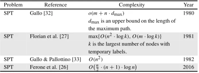
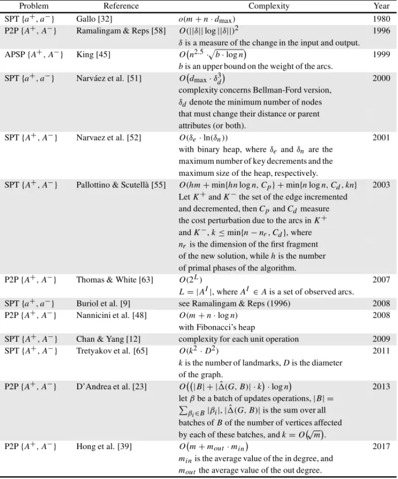
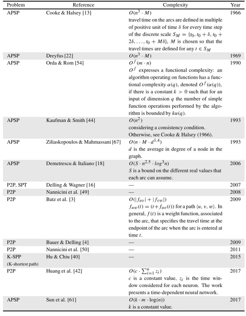
In this survey, starting from the origin till the current state of the art, two different kinds of shortest path problem on dynamic networks have been analyzed: reoptimization of shortest paths and time-dependent SPP. The onset of these problems can be traced back respectively to the works of Gallo [32] and Cooke & Halsey [13], both inspired by the seminal algorithm of Dijkstra [21] and Ford Jr [28] for the shortest path problem. In Tables 1, 2, and 3 the most relevant works are listed, respectively surveyed in this paper for root change, arc cost change and time dependent shortest path. More specifically, each table reports the problem in question, the reference, the computational complexity of the proposed algorithm (if specified), and the year of publication. For the three main problem categories,{P2P, SPT and APSP}, the following notations have been adopted:a+anda−are respectively used to indicate cost increase and decrease for a single arc, whileA+andA−are similarly used for batch updates, addressing respectively cost increase and decrease for a whole a set of arcs.
Table 1–Root change chronology. SPT indicates shortest path tree reoptimization.
Problem Reference Complexity Year
SPT Gallo [32] o(m+n·dmax) 1980
dmaxis an upper bound on the length of
the maximum path.
SPT Florian et al. [27] max{O(n2·logk),O(m·logk)} 1981 kis the largest number of nodes with
temporary labels.
SPT Gallo & Pallottino [33] O(n2) 1982 SPT Ferone et al. [26] On
2·(n+1)·logn
2016
Table 2–Arc cost change chronology.
Problem Reference Complexity Year
SPT{a+,a−} Gallo [32] o(m+n·dmax) 1980
P2P{A+,A−} Ramalingam & Reps [58] O(||δ||log||δ||)2 1996
δis a measure of the change in the input and output. APSP{A+,A−} King [45] O
n2.5· b·logn
1999 bis an upper bound on the weight of the arcs.
SPT{a+,a−} Narv´aez et al. [51] O
dmax·δ3d
2000 complexity concerns Bellman-Ford version,
δddenote the minimum number of nodes that must change their distance or parent attributes (or both).
SPT{A+,A−} Narvaez et al. [52] O(δe·ln(δn)) 2001 with binary heap, whereδeandδn are the
maximum number of key decrements and the maximum size of the heap, respectively.
SPT{A+,A−} Pallottino & Scutell`a [55] O(hm+min{hnlogn,Cp} +min{nlogn,Cd,kn} 2003 LetK+andK−the set of the edge incremented
and decremented, thenCpandCdmeasure the cost perturbation due to the arcs inK+ andK−,k≤min{n−nr,Cd}, where nr is the dimension of the first fragment of the new solution, whilehis the number of primal phases of the algorithm.
P2P{A+,A−} Thomas & White [63] O(2L) 2007
L= |AI|, whereAI ∈Ais a set of observed arcs. SPT{a+,a−} Buriol et al. [9] see Ramalingam & Reps (1996) 2008 P2P{A+,A−} Nannicini et al. [48] O(m+n·logn) 2008
with Fibonacci’s heap
SPT{A+,A−} Chan & Yang [12] complexity for each unit operation 2009 SPT{A+,A−} Tretyakov et al. [65] O(k2·D2) 2011
kis the number of landmarks,Dis the diameter of the graph.
P2P{A+,A−} D’Andrea et al. [23] O
|B| + | ˆ(G,B)| ·k ·logn
2013 letβbe a batch of updates operations,|B| =
βi∈B|βi|,| ˆ(G,B)|is the sum over all batches ofBof the number of vertices affected by each of these batches, andk=O√
m . P2P{A+,A−} Hong et al. [39] O
m+mout·min
2017 minis the average value of the in degree, and
Table 3–Time dependent chronology. Since the arcs have a time-depend cost in this case are considered
both the case of cost increasing and cost decreasing.
Problem Reference Complexity Year
APSP Cooke & Halsey [13] O(n3·M) 1966
travel time on the arcs are defined in multiple of positive unit of timeδfor every time step of the discrete scaleSM = {t0,t0+δ,t0+ 2δ, . . . ,t0+Mδ}, M is chosen so that the travel times are defined for anyt∈SM
APSP Dreyfus [22] O(n3·M) 1969
APSP Orda & Rom [54] Of(m·n) 1990
Of expresses a functional complexity: an algorithm operating on functions has a func-tional complexityα(q), denotedOf(α(q)), if there is a constantk >0 such that for an input of dimensionqthe number of simple function operations performed by the algo-rithm is bounded bykα(q).
APSP Kaufman & Smith [44] O(n2) 1993
considering a consistency condition. Otherwise, see Cooke & Halsey (1966).
APSP Ziliaskopoulos & Mahmassani [67] O(n·M·d1.4) 1993 dis the average in degree of a node in the graph.
APSP Demetrescu & Italiano [18] O(S·n2.5·log3n) 2006 Sis a bound on the different real values that each arc can assume.
P2P, SPT Delling & Wagner [16] — 2007
P2P Nannicini et al. [49] — 2008
P2P Batz et al. [3] O(|fuv| + |fvw|) 2009
fuw(t)=(t+fuv(t))for a pathu, v, w. In general,f(t)is a weight function, associated to the arc, that specifies the travel time at the endpoint of the arc when the arc is entered at timet.
P2P Bauer & Delling [4] — 2009
P2P Nannicini et al. [50] — 2011
K-SPP Hu & Chiu [40] — 2015
(K-shortest path)
P2P Huang et al. [42] O(c·n
i=1zi) 2017
cis a constant value, zi is the time win-dow considered for each neuron. The work presents a time-dependent neural network.
APSP Sun et al. [61] O(k·m·log(n)) 2017
Time-dependent SPP are shortest path problems whose arc cost function depends on both the arcs and the current instant belonging to a given time horizon. This line of research is of high interest given its suitability to model the occurrence of congestion in real transit planning scenar-ios. As indicated in the scientific literature, when the instance does not exhibit the FIFO property, the time-dependent SPP is NP-hard. Henceforth, in the near future it can be particularly appeal-ing to explore the possibility of the solution of such intractable instances, and preferably those arising from case studies, by means of heuristic and/or meta-heuristic techniques.
REFERENCES
[1] AHO A, HOPCROFT J & ULLMAN J. 1974. The design and analysis of computer algorithms. Addison-Wesley series in computer science and information processing. Addison-Wesley Pub. Co.
[2] AHUJARK, MAGNANTITL & ORLINJB. 1993. Network flows: theory, algorithms & applications. [3] BATZGV, DELLINGD, SANDERSP & VETTERC. 2009. Time-dependent contraction hierarchies.
In: Proceedings of the Meeting on Algorithm Engineering & Expermiments, pages 97–105. Society
for Industrial and Applied Mathematics.
[4] BAUERR & DELLINGD. 2009. Sharc: Fast and robust unidirectional routing.Journal of
Experi-mental Algorithmics (JEA),14(4).
[5] BAUERR, DELLINGD, SANDERSP, SCHIEFERDECKERD, SCHULTESD & WAGNERD. 2008. Combining hierarchical and goal-directed speed-up techniques for Dijkstra’s algorithm. In: Lecture Notes in Computer Science (including subseries Lecture Notes in Artificial Intelligence and Lecture
Notes in Bioinformatics), volume 5038 LNCS, pages 303–318.
[6] BAZARAAM & LANGLEYR. 1974. A dual shortest path algorithm.SIAM Journal on Applied
Math-ematics,26(3): 496–501.
[7] BELLMANR. 1958. On a routing problem.Quarterly of Applied Mathematics,16: 87–90.
[8] BERTSEKASDP. 1991. An auction algorithm for shortest paths.SIAM Journal on Optimization,1(4): 425–447.
[9] BURIOLLS, RESENDEMG & THORUPM. 2008. Speeding up dynamic shortest-path algorithms.
INFORMS Journal on Computing,20(2): 191–204.
[10] CERULLI R, FESTAP & RAICONIG. 2003. Shortest path auction algorithm without contractions using virtual source concept.Computational Optimization and Applications,26(2): 191–208.
[11] CHABINII & LAN S. 2002. Adaptations of the a* algorithm for the computation of fastest paths in deterministic discrete-time dynamic networks.IEEE Transactions on intelligent transportation
systems,3(1): 60–74.
[12] CHANEP & YANGY. 2009. Shortest path tree computation in dynamic graphs.IEEE Transactions
on Computers,58(4): 541–557.
[13] COOKEKL & HALSEYE. 1966. The shortest route through a network with time-dependent inter-nodal transit times.Journal of mathematical analysis and applications,14(3): 493–498.
[15] DELLING D & NANNICINIG. 2008. Bidirectional core-based routing in dynamic time-dependent road networks. In: International Symposium on Algorithms and Computation, pages 812–823. Springer.
[16] DELLING D & WAGNERD. 2007. Landmark-based routing in dynamic graphs. In: International
Workshop on Experimental and Efficient Algorithms, pages 52–65. Springer.
[17] DELLINGD, HOLZERM, M ¨ULLERK, SCHULZF & WAGNERD. 2009. High-performance multi-level routing. American Mathematical Society Providence, RI,74: 73–92.
[18] DEMETRESCU C & ITALIANO GF. 2006. Fully dynamic all pairs shortest paths with real edge weights.Journal of Computer and System Sciences,72(5): 813–837.
[19] DIALR, GLOVERF, KARNEYD & KLINGMAND. 1979. A computational analysis of alternative algorithms and labeling techniques for finding shortest path trees.Networks,9(3): 215–248.
[20] DIALRB. 1969. Algorithm 360: Shortest-path forest with topological ordering [h].Communications
of the ACM,12(11): 632–633.
[21] DIJKSTRAEW. 1959. A note on two problems in connexion with graphs.Numerische mathematik, 1(1): 269–271.
[22] DREYFUS SE. 1969. An appraisal of some shortest-path algorithms.Operations research,17(3): 395–412.
[23] D’ANDREAA, D’EMIDIOM, FRIGIONID, LEUCCIS & PROIETTIG. 2013. Dynamically main-taining shortest path trees under batches of updates. In: International Colloquium on Structural
Information and Communication Complexity, pages 286–297. Springer.
[24] ERTLG. 1998. Shortest path calculation in large road networks.OR Spectrum,20(1): 15–20. [25] FERONE D, FESTA P, GUERRIEROF & LAGANA` D. 2016. The constrained shortest path tour
problem.Computers & Operations Research,74: 64–77.
[26] FERONED, FESTAP, NAPOLETANOA & PASTORET. 2016. Reoptimizing shortest paths: From state of the art to new recent perspectives. In: Transparent Optical Networks (ICTON), 2016 18th
International Conference on, pages 1–5. IEEE.
[27] FLORIANM, NGUYENS & PALLOTTINOS. 1981. A dual simplex algorithm for finding all shortest paths.Networks,11(4): 367–378.
[28] FORDJRLR. 1956. Network flow theory. Technical report, DTIC Document.
[29] FORDJRLR & FULKERSONDR. 2015.Flows in networks. Princeton university press.
[30] FREDMANML & TARJANRE. 1987. Fibonacci heaps and their uses in improved network optimiza-tion algorithms.J. ACM,34(3): 596–615, July.
[31] FUL, SUND & RILETTLR. 2006. Heuristic shortest path algorithms for transportation applications: state of the art.Computers & Operations Research,33(11): 3324–3343.
[32] GALLOG. 1980. Reoptimization procedures in shortest path problem.Rivista di matematica per le
scienze economiche e sociali,3(1): 3–13.
[34] GOLDBERG AV & HARRELSONC. 2005. Computing the shortest path: A∗ search meets graph theory, pages 156–165.
[35] GUTMANRJ. 2004. Reach-based routing: A new approach to shortest path algorithms optimized for road networks.ALENEX/ANALC,4: 100–111.
[36] HART PE, NILSSONNJ & RAPHAELB. 1968. A formal basis for the heuristic determination of minimum cost paths.IEEE transactions on Systems Science and Cybernetics,4(2): 100–107.
[37] HILGERM, K ¨OHLERE, M ¨OHRINGRH & SCHILLINGH. 2009. Fast point-to-point shortest path computations with arc-flags.The Shortest Path Problem: Ninth DIMACS Implementation Challenge, 74: 41–72.
[38] HOLZERM, SCHULZF & WAGNERD. 2009. Engineering multilevel overlay graphs for shortest-path queries.Journal of Experimental Algorithmics (JEA),13: 5.
[39] HONGJ, PARKK, HANY, RASELMK, VONVOUD & LEEY-K. 2017. Disk-based shortest path discovery using distance index over large dynamic graphs.Information Sciences,382-383: 201–215.
[40] HUX & CHIUY-C. 2015. A Constrained Time-Dependent K Shortest Paths Algorithm Addressing Overlap and Travel Time Deviation.International Journal of Transportation Science and Technology, 4(4): 371–394.
[41] HUANGB, WUQ & ZHANF. 2007. A shortest path algorithm with novel heuristics for dynamic transportation networks.International Journal of Geographical Information Science,21(6): 625– 644.
[42] HUANGW, YAN C, WANGJ & WANGW. 2017. A delay neural network for solving time-dependent shortest path problem.Neural Networks,90: 21–28. ISSN 0893-6080.
[43] KANOULASE, DUY, XIAT & ZHANGD. 2006. Finding fastest paths on a road network with speed patterns. In: Data Engineering, 2006. ICDE’06. Proceedings of the 22nd International Conference on, pages 10–10. IEEE.
[44] KAUFMANDE & SMITHRL. 1993. Fastest paths in time-dependent networks for intelligent vehicle-highway systems application.Journal of Intelligent Transportation Systems,1(1): 1–11.
[45] KINGV. 1999. Fully dynamic algorithms for maintaining all-pairs shortest paths and transitive clo-sure in digraphs. InFoundations of Computer Science, 1999. 40th Annual Symposium on, pages 81– 89. IEEE.
[46] LAUTHERU. 2004. An extremely fast, exact algorithm for finding shortest paths in static networks with geographical background.Geoinformation und Mobilit¨at-von der Forschung zur praktischen
Anwendung,22: 219–230.
[47] M ¨OHRINGRH, SCHILLINGH, SCHUTZ¨ B, WAGNERD & WILLHALMT. 2007. Partitioning graphs to speedup dijkstra’s algorithm.Journal of Experimental Algorithmics (JEA),11: 2–8.
[48] NANNICINIG, BAPTISTEP, KROBD & LIBERTI L. 2008. Fast paths in dynamic road networks.
Proceedings of ROADEF,8: 1–14.
[49] NANNICINIG, DELLINGD, LIBERTIL & SCHULTESD. 2008. Bidirectional A* search for time-dependent fast paths. In: Lecture Notes in Computer Science (including subseries Lecture Notes in
[50] NANNICINIG, DELLING D, SCHULTESD & LIBERTI L. 2012. Bidirectional a* search on time-dependent road networks.Networks,59(2): 240–251.
[51] NARVAEZ´ P, SIUK-Y & TZENGH-Y. 2000. New dynamic algorithms for shortest path tree compu-tation.IEEE/ACM Transactions on Networking (TON),8(6): 734–746.
[52] NARVAEZP, SIUK-Y & TZENGH-Y. 2001. New dynamic spt algorithm based on a ball-and-string model.IEEE/ACM Transactions on Networking (TON),9(6): 706–718.
[53] NICHOLSONTAJ. 1966. Finding the shortest route between two points in a network.The computer
journal,9(3): 275–280.
[54] ORDA A & ROM R. 1990. Shortest-path and minimum-delay algorithms in networks with time-dependent edge-length.Journal of the ACM,37(3): 607–625.
[55] PALLOTTINOS & SCUTELLA` MG. 2003. A new algorithm for reoptimizing shortest paths when the arc costs change.Operations Research Letters,31(2): 149–160, mar 2003.
[56] PAPEU. 1974. Implementation and efficiency of moore-algorithms for the shortest route problem.
Mathematical Programming,7(1): 212–222.
[57] PUGLIESELDP & GUERRIEROF. 2013. A survey of resource constrained shortest path problems: Exact solution approaches.Networks,62(3): 183–200.
[58] RAMALINGAMG & REPST. 1996. An incremental algorithm for a generalization of the shortest-path problem.Journal of Algorithms,21(2): 267–305.
[59] SANDERSP & SCHULTESD. 2006. Engineering highway hierarchies. In:European Symposium on
Algorithms, pages 804–816. Springer.
[60] SCHULZF, WAGNERD & ZAROLIAGISC. 2002. Using multi-level graphs for timetable information in railway systems.Algorithm Engineering and . . .,00104: 43–59.
[61] SUNY, YUX, BIER & SONGH. 2017. Discovering time-dependent shortest path on traffic graph for drivers towards green driving.Journal of Network and Computer Applications,83: 204–212.
[62] TAKAOKAT. 1992. A new upper bound on the complexity of the all pairs shortest path problem.
Information Processing Letters,43(4): 195–199.
[63] THOMASBW & WHITECC. 2007. The dynamic shortest path problem with anticipation.European
Journal of Operational Research,176(2): 836–854.
[64] TOTHP & VIGOD. 2014.Vehicle routing: problems, methods & applications. SIAM.
[65] TRETYAKOVK, ARMAS-CERVANTESA, GARCIA´ -BANUELOS˜ L, VILO J & DUMASM. 2011. Fast fully dynamic landmark-based estimation of shortest path distances in very large graphs. In:
Proceedings of the 20th ACM international conference on Information and knowledge management,
pages 1785–1794. ACM.
[66] WAGNERD & WILLHALMT. 2003. Geometric speed-up techniques for finding shortest paths in large sparse graphs. In:European Symposium on Algorithms, pages 776–787. Springer.
[67] ZILIASKOPOULOSAK & MAHMASSANIHS. 1993. Time-dependent, shortest-path algorithm for real-time intelligent vehicle highway system applications.Transportation research record, pages 94–