Bayesian inference for the fitting of dry matter accumulation curves in garlic plants

(1)

Bayesian inference for the fitting of dry matter

accumulation curves in garlic plants

Leandro Roberto de Macedo(1)_{, Paulo Roberto Cecon}(2)_{, Fabyano Fonseca e Silva}(3)_{, Moysés Nascimento}(2)_, Guilherme Alves Puiatti(2)_{, Ana Carolina Ribeiro de Oliveira}(2)_{and Mario Puiatti}(4)

(1)_{Universidade Federal de Juiz de Fora, Departamento de Economia, Campus Governador Valadares, Avenida Dr. Raimundo M.} Rezende, no_{330, Centro, CEP 35010-177 Governador Valadares, MG, Brazil. E-mail: leandro.macedo@ufjf.edu.br}(2)_Universidade Federal de Viçosa (UFV), Departamento de Estatística, Avenida P.H. Rolfs, s/no_{, CEP 36570-900 Viçosa, MG, Brazil. E-mail:} cecon@ufv.br, moysesnascim@ufv.br,guilherme@dpi.ufv.br, kroll_olliveira@hotmail.com (3)_{UFV, Departamento de Zootecnia, Avenida} P.H. Rolfs, s/no_{, CEP 36570-900 Viçosa, MG, Brazil. E-mail: fabyanofonseca@ufv.br}(4)_{UFV, Departamento de Fitotecnia, Avenida P.H.} Rolfs, s/no_{, CEP 36570-900 Viçosa, MG, Brazil. E-mail: mpuiatti@ufv.br}

Abstract – The objective of this work was to identify nonlinear regression models that best describe dry matter accumulation curves over time, in garlic (Allium sativum_{) accessions, using Bayesian and frequentist} approaches. Multivariate cluster analyses were made to group similar accessions according to the estimates

of the parameters with biological interpretation (β1 and β3). In order to verify if the obtained groups were equal, statistical tests were applied to assess the parameter equality of the representative curves of each group. Thirty garlic accessions were used, which are kept by the vegetable germplasm bank of Universidade Federal

de Viçosa, Brazil. The logistic model was the one that fit best to data in both approaches. Parameter estimates

of this model were subjected to the cluster analysis using Ward’s algorithm, and the generalized Mahalanobis distance was used as a measure of dissimilarity. The optimal number of groups, according to the Mojena method, was three and four, for the frequentist and Bayesian approaches, respectively. Hypothesis tests for the

parameter equality from estimated curves, for each identified group, indicated that both approaches highlight the differences between the accessions identified in the cluster analysis. Therefore, both approaches are

recommended for this kind of study.

Index terms: Allium sativum_{, cluster analysis, multivariate clustering curves, nonlinear models.}

Inferência bayesiana para o ajuste de curvas do

acúmulo de matéria seca em plantas de alho

Resumo – O objetivo deste trabalho foi identificar modelos de regressão não linear que melhor descrevam

curvas de acúmulo de matéria seca em acessos de alho (Allium sativum_{), ao longo do tempo, com uso das} abordagens bayesiana e frequentista. Análises de agrupamento multivariadas foram empregadas para agrupar

acessos similares quanto às estimativas dos parâmetros das curvas com interpretação biológica (β1 e β3).

Para verificar se os grupos formados eram iguais, aplicaram-se testes estatísticos para testar a igualdade

de parâmetros das curvas representativas de cada grupo. Foram utilizados 30 acessos de alho, mantidos pelo Banco de Germoplasma de Hortaliças da Universidade Federal de Viçosa. O modelo logístico foi o que melhor se ajustou aos dados em ambas as abordagens. As estimativas dos parâmetros deste modelo foram submetidas à análise de agrupamento com o algoritmo de Ward, e a distância generalizada de Mahalanobis

foi utilizada como medida de dissimilaridade. O número ótimo de grupos, de acordo com o método de Mojena, foi de três e quatro para as abordagens frequentista e bayesiana, respectivamente. Testes de hipótese

quanto à igualdade de parâmetros das curvas estimadas, para cada grupo de acesso, indicaram que ambas

as metodologias evidenciam as diferenças identificadas pela análise de agrupamento. Portanto, ambas as abordagens são indicadas para estudos desta natureza.

Termos para indexação: Allium sativum_{, análise de agrupamento, agrupamento multivariado de curvas,}

modelos não lineares.

Introduction

Garlic (Allium sativum_{L.), the fourth most}

economically important vegetable in Brazil, is

cultivated in most regions of the country (Mota et al., 2006; Lucini, 2008). In addition to its culinary use, garlic also stands out for its medicinal qualities, such as

(2)

antifungal, antiviral, diuretic, and antioxidant properties, besides being an immune system stimulant (Trani, 2009).

The study on the curves of plant growth and dry matter accumulation of garlic allows to detect problems on the development of the culture (Reis et al., 2014), which contributes to a proper management. According to Pôrto et al. (2007), the curves of dry matter and nutrient accumulation are useful as an indication for care demands in each stage of plant development.

Nonlinear regression models have been shown as adequate to describe these curves, both by the frequentist and by the Bayesian approaches, which have parameters with biological interpretation, such as asymptotic weight and growth velocity (Martins Filho et al., 2008). Puiatti et al. (2013) and Reis et al.

(2014) indicated high-fitting quality for the logistic,

Gompertz, and Von Bertalanffy models, in garlic accessions, using the frequentist approach. However, there are no reports about these models in garlic accessions using the Bayesian approach.

The Bayesian inference considers the vectors of unknown parameters as random quantities, and any initial information on them can be represented by probabilistic models. Thus, by attributing probability distributions, the Bayesian approach allows to incorporate some knowledge on these parameters before data have been collected. Therefore, to perform a Bayesian inference, it is necessary to

specify an a priori probability density function P(θ)

that combined with the likelihood L(y1, ..., yn|θ), by means of the Bayes’ theorem, generates the a

posteriori probability density function P(θ|Yn). Any

conclusion on the θ parameter is performed from the a

posteriori density distribution, which is represented as

P Y L Y P

L Y P d

n

n n

θ θ θ

(

)

=

(

)

( )

(

)

( )

∫

,

in which Yn = {y1, ..., yn}.

According to Rosa (1998), to infer on any element of θ,

it is necessary to incorporate the a posteriori integrated

distribution of the parameters – P(θ1|Y) – over all other

parameters. Thus, to make inference on θ1, it is necessary

to obtain the P(θ1|Y) distribution, which is called the posterior marginal distribution, represented by

P θ₁Y P θ Y dθ

θ θ

(

)

=

(

)

≠

∫

1

1.

The integrals to obtain the marginal distributions usually does not have analytical solutions, which makes it necessary to use specialized iterative algorithms such as the Gibbs sampler and the Metropolis-Hastings, which are called Markov chain Monte Carlo (MCMC) algorithms.

Usually, in growth curve studies, the researcher is interested in comparing the estimates of the growth curve parameters among the different populations, in order to identify in which one the growth process was

most efficient (Silveira et al., 2011). The cluster analysis

allow to group individuals with great homogeneity, but with high heterogeneity among them (Johnson & Wichern, 1992; Azevedo et al., 2012; Faria et al., 2012). Therefore, it is possible to group the garlic varieties according to the studied variables, such as the growth rate and dry matter accumulation, derived from the growth curve.

The objective of this work was to identify nonlinear regression models that best describe dry matter accumulation curves over time, in garlic accessions, using the Bayesian and frequentist approaches, and to infer on the estimated curve equality for each group

identified by both approaches.

Materials and Methods

The field experiment was carried out from March

to November in 2010, in an area belonging to Plant Science Department of the Universidade Federal de Viçosa (20º45'S, 42º51'W, at 650 m altitude), in the Zona da Mata region, state of Minas Gerais, Brazil.

Thirty garlic accessions, registered in the vegetable germplasm bank of Universidade Federal de Viçosa (VGB/UFV), were evaluated (Table 1). A randomized complete block design was used, considering four replicates, and plots were constituted by four longitudinal rows of 1.0 m length. The planting spacing was 0.25×0.10 m, which resulted in 40 plants per plot. The total dry matter evaluation was performed in four periods: 60, 90, 120, and 150 days after planting (DAP). The models used to describe the longitudinal trajectory of the total dry matter accumulation are shown in Table 2, where: β1 is the parameter that represents the asymptotic weight; β2 represents the

(3)

the dependent variable; Xi is the independent variable;

and εi is the random error, with εi ~ N(0, σ2).

For the Bayesian approach, estimates of the growth curve parameters were obtained by a hierarchical method, which was adjusted separately for each of the seven models tested. As an example for the logistic model, the Bayesian methodology was applied

regarding the following specifications:

a) Sample data distribution,

yij e N i i itij e

i i i

θ σ β β β σ

θ β β β

, ~ exp , ,

, , 2

1 2 3

1 2

1 2 3

1+

(

−

)

  

(

)

=

(

)

− ;;

b) Likelihood function,

L y Z

in which Z

e i N j n e e θ σ πσ σ

, 2 exp

1 1 2

2 2 1 2 2

(

)

∝ ∏ ∏ _−

[ ]

     = =

==y_ij −β₁_i_1+β₂_iexp

(

−β₃_{i ij}t

)

_−1;

and c) a priori distribution,

β1i~N

(

µ τβ1, β1

)

; β2i~N

(

µ τβ2, β2

)

; β3i~N

(

µ τβ3, β3

)

; and

σ µ τ

σ σ

e G

e e

2

2 2

~

(

,

)

,_{in which:}σe τe

2 1

= ; and τ_{e is the error}

variance.

In the last stage, the values for the parameters considered for the previous distributions were

specified: µβk N µµβk τµβk

~

(

,

)

, τβk~N

(

αβk,ββk

)

, in which

k = 1, 2, and 3. These values were respectively considered as equal to the mean and the variance of the parameter estimates reported in previous studies (Puiatti et al., 2013; Reis et al., 2014) with the same accessions.

The presented Bayesian inference was implemented in the R software (R Core Team, 2015), by the R2OpenBugs pack, in which the Gibbs sampler and the Metropolis–Hastings algorithms were implemented. For all models, 20,000 iterations were used, from which

the first 1,000 were discarded to avoid errors associated

with the initial values. To ensure sample independence, the sampling interval of four iterations was used. In

this way, a final chain of 4,000 observations for each

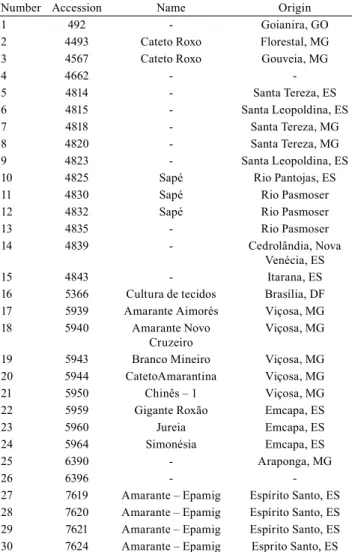
Table 1. The 30 garlic (Allium sativum_{) accessions used in} this study, which are registered in the Vegetable Germplasm Bank of Universidade de Viçosa.

Number Accession Name Origin

1 492 - Goianira, GO

2 4493 Cateto Roxo Florestal, MG

3 4567 Cateto Roxo Gouveia, MG

4 4662 -

-5 4814 - Santa Tereza, ES

6 4815 - Santa Leopoldina, ES

7 4818 - Santa Tereza, MG

8 4820 - Santa Tereza, MG

9 4823 - Santa Leopoldina, ES

10 4825 Sapé Rio Pantojas, ES

11 4830 Sapé Rio Pasmoser

12 4832 Sapé Rio Pasmoser

13 4835 - Rio Pasmoser

14 4839 - Cedrolândia, Nova

Venécia, ES

15 4843 - Itarana, ES

16 5366 Cultura de tecidos Brasília, DF

17 5939 Amarante Aimorés Viçosa, MG

18 5940 Amarante Novo

Cruzeiro

Viçosa, MG

19 5943 Branco Mineiro Viçosa, MG

20 5944 CatetoAmarantina Viçosa, MG

21 5950 Chinês – 1 Viçosa, MG

22 5959 Gigante Roxão Emcapa, ES

23 5960 Jureia Emcapa, ES

24 5964 Simonésia Emcapa, ES

25 6390 - Araponga, MG

26 6396 -

-27 7619 Amarante – Epamig Espírito Santo, ES

28 7620 Amarante – Epamig Espírito Santo, ES

29 7621 Amarante – Epamig Espírito Santo, ES

30 7624 Amarante – Epamig Esprito Santo, ES

Table 2. Nonlinear regression models used to describe the dry matter accumulation in garlic (Allium sativum_{) plants.}

Model Function

Gompertz (G)

yi e i

e xi = − + − ( )        

β β ε

β

1

2 3

Logístico (L) y

e i= + (− xi) + i

β

β β ε

1 2

1 3

Meloun I (M1) yi e

x i

i

= − (− )+ β β β ε

1 2

3

Meloun II (M2) yi e

x i

i

= − (− − )+ β β β ε

1

2 3

Brody (B) yi e

x i

i

=

(

− (− )

)

+

β β β ε

1 1 2

3

Von Bertalanffy (vB) yi e

x i

i

=

(

− (− )

)

+

β β β ε

1 2

3

1 3

Mitscherlich (M) yi e

x i

i

=

(

− ( − )

)

+

β β β β ε

1 1

(4)

parameter was obtained. To assess the convergence, the tests of Geweke and of Raftery-Lewis (1992) were used by means of the Bayesian output analysis (BOA) package of the R software (R Core Team, 2015).

For the frequentist approach, the parameters were estimated using the method of ordinary least squares, with solutions obtained by the Gauss–Newton iterative process through the nls of the R package. To evaluate

the fitting quality of the models, the convergence

percentage (C%), the mean square error (MSE),

the coefficient of determination (R2_{), the Akaike´s} information criterion (AIC), the Bayesian information criterion (BIC), and the mean absolute deviation (MAD) were used for the frequentist approach; whereas the deviance information criterion (DIC) was used for the Bayesian approach.

After choosing the best model, in each approach, the parameter estimates were grouped using the Ward algorithm, with the aim of grouping the most similar accessions. The method proposed by Ward Jr. (1963) is based on the variation changes within and among groups undergoing formation at each step of the grouping process. The measure utilized was the generalized distance of Mahalanobis, which considers the existence of correlations among the analyzed characteristics, and shows differences of scales among the variables. To determine the number of groups, the procedure suggested by Mojena (1977) was used, and the adopted constant value for k was 1.25.

The accession classifications in groups by the

cluster analysis was made by estimates obtained from equations that represented the curves related to each group. The next step was to test the hypotheses for the parameter equality of these models in relation to the formed groups. For the frequentist approach, the model identity method for nonlinear regression, presented by Regazzi & Silva (2010), was used. Therefore, to check the equality of the parameter estimates in the accession groups, the F-test was used to evaluate the

hypothesis which states that the reduced model, fitted for both groups, is identical to the fitted complete

model, according to F(H0) = {[SQRR(ω) - SQRR(Ω)]/

[t(r - 1)]}/ {[SQRR(Ω)]/ [N - Hp - H(r - 1)]}, in which SQRR represents the residual sum of squares of the

regression for the given model; Ω is the parametric space for the complete model; ω is the parametric

space for the reduced model under H0; t is the number

of parameters to be tested; and N is the total number of observations.

The considered hypotheses were as follows: H0(1) : β

1(1) = β1(2) = ... = β1(k) = β1 vs HA(1) : not all β1k are equal;

H0(2) : β

3(1) = β3(2) = ... = β3(k) = β3 vs HA(2) : not all β3k are equal;

H0(3) : β

1(1) = β1(2) = ... = β1(k) = β1 and β3(1) = β3(2) = ... =

β3(k) = β3 vs HA(3) : not H0(3), in which k is the number of formed groups.

For the Bayesian approach, the equality tests of the parameters of the models, in relation to the formed groups, were performed using samples obtained from the a posteriori marginal distributions related to differences between the estimates β1 and



β3 for all

groups. Thus, the differences showed themselves as an additional parameter in the model, and they allowed to test the hypothesis of the equality of parameters through the highest posterior density (HPD). If the value zero is contained in the interval, it is quite conclusive that the parameters for the two populations involved in the contrast are statistically identical. This methodology was proposed by Silva et al. (2005), to compare curve parameters for the lactation of goats from two populations. Afterwards, it was used to compare the growth curves of Nelore cattle from different genetic groups (Silva et al., 2007).

Results and Discussion

In the frequentist approach, the means and the standard deviations of the evaluated parameters for

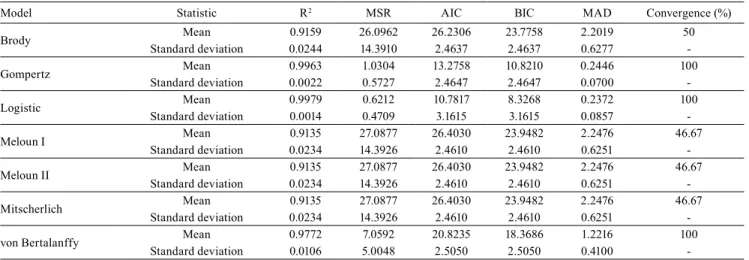
the fitting quality of the models did not allow the differentiation of the models classification (Table 3);

that is, the models with the lowest values for MSE, AIC, BIC, and MAD were also those that showed the highest values for R2. The model that best fitted to the data was the logistic (L) model, followed by the Gompertz (G), Von Bertalanffy (vB), Brody (B), Meloun I (M1), Mitscherlich (M), and Meloun II (M2). Reis et al. (2014), studying nonlinear regression models to describe the dry matter accumulation in different parts of the garlic plant, found that the L model was

the one that best fitted the data for all plant parts

evaluated. A similar result was reported by Puiatti et

al. (2013), who identified and grouped the nonlinear regression models that best fitted the description of

(5)

time, where L showed better performance than that of the B, G, L, M, M1, M2, vB, and Meloun III models.

The L model fitted the data well in several experiments

with nonlinear regression models, for the description of growth curves or nutrient accumulation, as in Pôrto et al. (2007) for onion cultivation, Maia et al. (2009) for banana trees, and Martins Filho et al. (2008) who also reported great adjustments for the L model using the Bayesian methodology for the growth data of two bean cultivars.

Among the analyzed models, the only ones that showed convergence for all the accessions were the L, G, and vB models. For the B model, there was convergence for half the accessions. This outcome

possibly occurred because this model has no inflection

point, which hinders its performance in this sort of study, since these data have a sigmoid format.

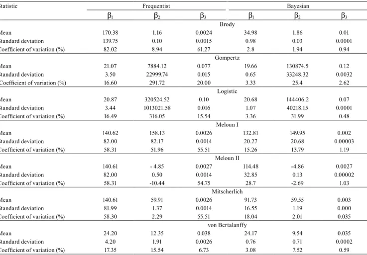
Means, standard deviations, and variation

coefficients of the parameter estimates for each model,

in both approaches, are shown in Table 4. As for the



β1 estimates, for the frequentist approach, the B, M1,

M2, and M models were not good representatives for curves of total dry matter accumulation, since the values of these estimates were very high in relation

to the final garlic plant weight. According to Reis et

al. (2014), β1 and



β3 are practically the same in the

B, M1, M2, and M models. This characteristic may result from the fact that these models are only different

reparameterizations of the same model, in which the changes of values for the estimates occur only for the

β2 parameter. However, the L, G, and vB models are good representatives of the obtained results in this kind of study, and showed β1 estimate values quite

close to the reality of the data.

The β2 estimate was quite different in all models,

whose lowest value (-4.85) was observed for the M2 model, and the highest value (320,524.5) for the L model. This result, however, does not constitute a problem, since such parameter does not have a biological interpretation, and it is only a location parameter. The G, vB, B, M1, M, and M2 models had the lowest β3 estimate values that were all very close

to one another. The L model had the highest value for

the estimate and showed a very defined sigmoid shape.

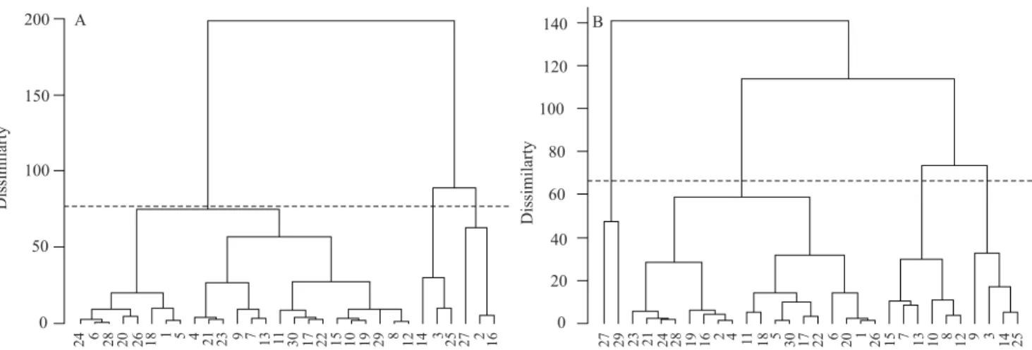
After grouping the β1 and



β3 estimates of the L

model, using the Mojena method, an optimum number of three groups was obtained, and the cutoff point in the dendrogram was 75.1, which corresponds to 37% of the maximum distance observed in fusion levels

(Figure 1). The accessions were classified as follows:

group I, 1, 4, 5, 6, 7, 8, 9, 10, 11, 12, 13, 15, 16, 17, 18, 19, 20, 21, 22, 23, 24, 26, 28, 29 and 30; group II, 3, 14, and 25; group III, 2, 16, and 27.

After the group classification of the accessions, a

curve was adjusted for each group in the model that

Table 3. Means of the determination coefficient (R2_{), of the mean squared residue (MSR), of the Akaike information} criterion (AIC), of the Bayesian information criterion (BIC), and of the mean absolute deviation of residues (MAD) of the adjusted models for the mean of total dry matter of plant (TDMP) of the 30 garlic (Allium sativum_{) accessions analyzed, with} the respective convergence for each model.

Model Statistic R2 _MSR _AIC _BIC _MAD _{Convergence (%)}

Brody Mean 0.9159 26.0962 26.2306 23.7758 2.2019 50

Standard deviation 0.0244 14.3910 2.4637 2.4637 0.6277

-Gompertz Mean 0.9963 1.0304 13.2758 10.8210 0.2446 100

-Logistic Mean 0.9979 0.6212 10.7817 8.3268 0.2372 100

-Meloun I Mean 0.9135 27.0877 26.4030 23.9482 2.2476 46.67

-Meloun II Mean 0.9135 27.0877 26.4030 23.9482 2.2476 46.67

-Mitscherlich Mean 0.9135 27.0877 26.4030 23.9482 2.2476 46.67

-von Bertalanffy Mean 0.9772 7.0592 20.8235 18.3686 1.2216 100

(6)

-best fitted the data (L), and the following equations

were obtained for the groups I, II, and III, respectively:

ŷ = 20.31[1 + 27442.4exp(-0.098x)]-1

ŷ = 18.47[1 + 856629.5exp(-0.136x)]-1_{, and}

ŷ = 27.49[1 + 79138.1exp(-0.107x)]-1_.

As the H0(3) was significant (Table 5), we conclude that at least one of the estimates differs from the others; therefore, a single equation cannot be adopted for the three groups. Nonetheless, it is pointed out that

the hypothesis that the β3 parameter value is the same for the three groups was not rejected. Thus, a new

two-against-two comparison was made to estimate the β1 parameter, to check which equations were statistically equal. Based on the evaluated hypotheses, only the asymptotic weight estimates for groups I and II were equal (for H0(5)_{, p<0.01, and for H0}(4)_{, p>0.01). Thus, it} can be concluded that the equations of the groups I

and II do not significantly differ, and that they can be

represented by one single model. Therefore, only two

equations are sufficient to represent the accessions,

one for groups I and II, and another for group III, as follows:

ŷ = 20.10[1 + 35386.9exp(-0.10x)]-1_and

ŷ = 27.31[1 + 39820.17exp(-0.10x)-1_{, respectively.} Using these two adjusted equations, it is possible to conclude that the mean asymptotic weight of the accessions (27.31 g) of group III was superior to those of the other accessions (20.10 g), which is an evidence that these accessions show higher dry matter accumulation at 150 DAP. As for the β3 estimate, there were no significant differences, which indicates that,

theoretically, the analyzed variations have the same growth rate.

Table 4.Mean, standard deviation, and coefficient of variation of the estimates of β1, β2, and β3 parameters, for the adjusted

models with the frequentist and Bayesian approaches.

Statistic Frequentist Bayesian

β1 β2 β3 β1 β2 β3

Brody

Mean 170.38 1.16 0.0024 34.98 1.86 0.01

Standard deviation 139.75 0.10 0.0015 0.98 0.03 0.0001

Coefficient of variation (%) 82.02 8.94 61.27 2.8 1.94 0.94

Gompertz

Mean 21.07 7884.12 0.077 19.66 130874.5 0.12

Logistic

Mean 20.87 320524.52 0.10 20.68 144406.2 0.07

Meloun I

Mean 140.62 158.13 0.0026 132.81 149.95 0.002

Meloun II

Mean 140.61 - 4.85 0.0027 114.48 -4.86 0.0027

Coefficient of variation (%) 58.31 -10.44 54.75 28.7 -2.69 1.03

Mitscherlich

Mean 140.61 59.91 0.0026 91.73 59.55 0.003

von Bertalanffy

Mean 24.20 12.35 0.038 24.17 9.54 0.035

(7)

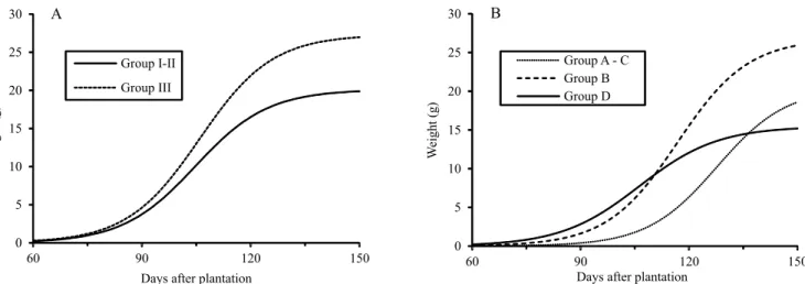
The total dry matter accumulation curves were adjusted by the L model for each of the two equations through the frequentist approach (Figure 2). The curve for group III was superior to that for groups I and II, irrespective of time. The two curves reached the asymptotic weight around 130 DAP; that is, after this time, the weight tends to stabilize, and the plants

are ready to be harvested without any significant yield

loss.

For the Bayesian approach, the convergence was reached for all models, according to the convergence tests of Raftery & Lewis, Heidelberger & Welch, and Geweke (Raftery & Lewis, 1992), since the heating period (“burn in”), the total number of iterations, and the distance among samples (“thin”) were superior to the minimum recommended by Raftery & Lewis (1992). Furthermore, all values for the dependency

factor (DF) of the criterion were close to 1. According to the authors, it can be said that the chain did not reach convergence when DF was superior to 5.0. The Heidelberger & Welch criterion showed acceptance of the null hypothesis of chain stationarity, making a higher number of iterations unnecessary. For the Geweke criterion, all the obtained p-values were

superior to the established significance level of 0.5,

and, therefore, they did not provide evidence against the convergence.

The DIC values were 322.2, 448.4, 531.9, 572.7, 672.7, 685.9, and 725 for the L, G, vB, M2, M1, M, and B models, respectively. It should be noted that

the L model was the one that best fitted to the data,

with the lowest value, which is in accordance with the results obtained by the frequentist approach, and also with the results reported by Puiatti et al. (2013) and

Figure 1. Dendrogram obtained from the grouping of the estimates for β1 and β3 parameters of the logistic model, with the

30 garlic (Allium sativum_{) accessions analyzed by the frequentist (A) and Bayesian (B) approaches.}

Table 5. Analyzed hypotheses, statistical values for the F test, number of degrees of freedom, and descriptive level (p-value) of the parameter equality tests by the frequentist approach.

Hypothesis df F p-value

H0(1) : β1(1) = β1(2) = β1(3) = β1 vs HA(1) : not H0(1) 1 and 113 26.6 3.3x10-10

H0(2) : β3(1) = β3(2) = β3(3) = β3 vs HA(2) : not H0(2) 1 and 113 0.39 0.6724

H0(3) : β1(1) = β1(2) = β1(3) = β1 and β3(1) = β3(2) = β3(3) = β3 vs HA(3) : not H0(3) 2 and 113 16.6 9.8x10-10

H0(4) : β1(1) = β1(2) = β1 vs HA(4) : not H0(4) 2 and 103 1.04 0.31

H0(5) : β1(1) = β1(3) = β1 vs HA(5) : not H0(5) 2 and 103 72.5 1.4 x10-13

(8)

Reis et al. (2014). After the L model, those which best

fitted to the data were the G, vB, M2, M1, M, and B

models; however, M2, M1, M and B differ from the

classification obtained with the frequentist approach.

To make the adjustments obtained with the two

methods comparable, determination coefficients were

calculated for the Bayesian approach from the square correlation between the observed and the predicted values. The results were similar to those obtained with the frequentist approach; thus, the L model showed the highest R2 _{value (0.99).}

All the estimated values by the Bayesian approach

showed a lower coefficient of variation value than

those estimated by the frequentist approach (Table 4). Moreover, all the estimates of asymptotic weight for the same model, in the frequentist approach, were superior to those found with the Bayesian approach. As for the β1 estimate, the M1, M2, and M models,

similarly to the frequentist approach, were not good representatives for the data standard behavior in this kind of study, since the value for these estimates was

very high in relation to the total final weight of plants.

Nevertheless, the L, G, and vB models were good representatives.

The grouping of the β1 and



β1 estimates of the

parameters for the L model in the Bayesian approach, by the Mojena criterion with k= 1.25, indicated the optimum number of four groups. The cutoff point in the dendrogram was 66.4, which corresponds to 47.1% of the maximum distance observed at different levels

of fusion (Figure 1). The accessions were classified as

follows: group A, 1, 2, 4, 5, 6, 11, 16, 17, 18, 19, 20, 21, 22, 23, 24, 26, 28, and 30; group B, 3, 9, 14, and 25; group C, 7, 8, 10, 12, 13, and 15; and group D, 27 and 29.

After the accession classifications into groups, a

curve for each group was adjusted in the model that

best fitted to data (L model) in the Bayesian analysis,

and the following equations were obtained:

ŷ = 20.14[1 + 72690.2exp(-0.107x)]-1_,

ŷ = 26.82[1 + 151335.5exp(0.102x)]-1_,

ŷ = 21.4[1 + 17552.9exp(-0.092x)]-1_{, and}

ŷ = 15.47[1 + 5770.5exp(-0.085x)]-1_{, for groups A, B,} C, and D, respectively.

Groups A and C did not differ from one another statistically (Table 6), since the HPD interval had a value of zero both for the asymptotic weight and for the growth rate. The remaining differences were all

significant. Thus, the accessions can be classified into

three groups, in which groups A and C are considered one single group, the A–C group. Therefore, the adjusted equations to represent groups A–C, B, and D were, respectively:

ŷ = 20.46[1 + 54919.6exp(-0.1035x)]-1_,

ŷ = 26.81[1 + 151335.6exp(-0.1021x)]-1_{, and}

ŷ = 15.47[1 + 17553.0exp(-0.092x)]-1_.

We conclude, therefore, that the mean asymptotic weight of the accessions in group B is superior to those of the other groups, which is an evidence that the accessions in this group show a higher dry

(9)

matter accumulation per asymptotic weight. Except for the access 9, the other ones from the group of higher asymptotic weight, by the Bayesian approach, coincided with those observed in the frequentist approach. As for the group with the lowest weight, the

only accession that was classified in both approaches

was the number 27. The A–C group had the higher number of accessions (24), with a 20.46 g mean asymptotic weight, which is very close to that in group I–II in the frequentist approach (20.10 g).

The estimated asymptotic weight for the group with the highest weight in the frequentist approach was superior to that estimated in the Bayesian one. The asymptotic weight estimated for the group with the lowest weight showed also the same behavior. The Bayesian approach was less rigorous at classifying the groups.

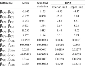
Approximately from 125 DAP, the curve for group B was superior to those of the other groups (Figure 2), whereas the curve for group D was the lowest one from 110 DAP on. This is an evidence that the group B is formed by latter varieties. Thus, if it is desirable to harvest the plants before 125 DAP, the variables in group A–C are recommended. However, if the harvest is to occur after this date, the variables in group B will produce a higher weight. This interpretation from a practical perspective is useful to justify research in the

phytotechnology field that involves the estimation of

curves by nonlinear models with posterior grouping, and the application of hypothesis tests to compare the generated curves for each group.

Conclusions

1. The logistic model is that which fits best to the

yield data of total dry matter of garlic(Allium sativum₎

plants, in the evaluated 30 accessions, by both the frequentist and Bayesian approaches.

2. The hypothesis tests for the parameter equality of the estimated curves, for each group of accessions, indicate that both methods show the same differences reported by the clustering analysis, which makes them both indicated for experiments of this nature.

Acknowledgments

To Coordenação de Aperfeiçoamento de Pessoal

de Nível Superior (Capes), to Conselho Nacional de

Desenvolvimento Científico e Tecnológico (CNPq), and to Fundação de Amparo à Pesquisa do Estado de Minas Gerais (Fapemig), for financial support.

References

AZEVEDO, C.F.; SILVA, F.F. e; RIBEIRO, N.B.; SILVA, D.J.H.

da; CECON, P.R.; BARILI, L.D.; PINHEIRO, V.R. Classificação

multivariada de curvas de progresso da requeima do tomateiro entre acessos do Banco de Germoplasma de Hortaliças da UFV.

Ciência Rural, v.42, p.414-417, 2012. DOI: 10.1590/S0103-84782012000300005.

FARIA P.N.; CECON P.R.; SILVA, A.R. da; FINGER F.L.; SILVA, F.F. e; CRUZ C.D.; SÁVIO F.L. Métodos de agrupamento em estudo de divergência genética de pimentas. Horticultura Brasileira. v.30, p.428-432, 2012. DOI: 10.1590/S0102-05362012000300012.

JOHNSON, R.A.; WICHERN, D.W. Applied multivariate statistical analysis. 3rd_{ed. New Jersey: Prentice Hall, 1992. 642p.}

LUCINI, M.A. Alho roxo no Brasil: um pouco da história dos

números desse nobre. Revista Nosso Alho, ed.1, p.16-21, 2008.

MAIA, E.; SIQUEIRA, D.L. de; SILVA, F.F. e; PETERNELLI,

L.A.; SALOMÃO, L.C.C. Método de comparação de modelos de regressão não-lineares em bananeiras. Ciência Rural, v.39, p.1380-1386, 2009. DOI: 10.1590/S0103-84782009000500012.

MARTINS FILHO, S.; SILVA, F.F. e; CARNEIRO, A.P.S.; MUNIZ, J.A. Abordagem Bayesiana das curvas de crescimento de duas cultivares de feijoeiro. Ciência Rural, v.38, p.1516-1521, 2008. DOI: 10.1590/S0103-84782008000600004.

Table 6. Mean, standard deviation, and a posteriori maximum density interval (HPD) of 95% for the estimate differences of β1 parameters, and the estimate differences

of β3 parameters, in all groups, by the Bayesian approach.

Difference Mean Standard

deviation

HPD

Inferior limit Upper limit

β1(A) – β1(B) -6.645 1.155 -8.93 -4.37

β1(A) – β1(C) -0.973 0.858 -2.67 0.68

β1(A) – β1(D) 4.584 0.981 2.68 6.51

β1(B) – β1(C) 5.673 1.334 3.07 8.33

β1(B) – β1(D) 11.230 1.415 8.46 14.03

β1(C) – β1(D) 5.557 1.194 3.21 7.89

β3(A) – β3(B) 0.00522 0.000563 0.0042 0.0063

β3(A) – β3(C) 0.000367 0.000565 -0.0008 0.0014

β3(A) – β3(D) 0.0219 0.000411 0.02119 0.02277

β3(B) – β3(C) -0.00485 0.000563 -0.0061 -0.0039

β3(B) – β3(D) 0.0167 0.000411 0.01598 0.01758

(10)

MOJENA, R. Hierarchical grouping methods and stopping rules: an evaluation. Computer Journal, v.20, p.359-363, 1977. DOI: 10.1093/comjnl/20.4.359.

MOTA, J.H.; YURI, J.E.; RESENDE, G.M.; SOUZA, R.J. de. Similaridade genética de cultivares de alho pela comparação de caracteres morfológicos, físico-químicos, produtivos e

moleculares. Horticultura Brasileira, v.24, p.156-160, 2006. DOI: 10.1590/S0102-05362006000200006.

PÔRTO, D.R. de Q.; CECILIO FILHO, A.B.; MAY, A.; VARGAS,

P.F. Acúmulo de macronutrientes pela cultivar de cebola 'Superex' estabelecida por semeadura direta. Ciência Rural, v.37, p.949-955, 2007. DOI: 10.1590/S0103-84782007000400005.

PUIATTI, G.A.; CECON, P.R.; NASCIMENTO, M.; PUIATI, M.; FINGER, F.L.; SILVA, A.R. da; NASCIMENTO, A.C.C.

Análise de agrupamento em seleção de modelos de regressão não

lineares para descrever o acúmulo de matéria seca em plantas de alho. Revista Brasileira de Biometria, v.31, p.337-351, 2013. R CORE TEAM. R: a language and environment for statistical computing. Vienna: R Foundation for Statistical Computing, 2015. Available at: <http://www.r-project.org/>. Accessed on: Sept. 14 2015.

RAFTERY, A.E.; LEWIS, S. How many iterations in the Gibbs

sampler? In: BERNARDO, J.M; BERGER, J.O.; DAWID, A.P.; SMITH, A.F. M. (Ed.). Bayesian statistics 4: proceedings of the Fourth Valencia International Meeting. Oxford: University Press, 1992. p.763-773.

REGAZZI, A.J.; SILVA, C.H.O. Testes para verificar a igualdade de parâmetros e a identidade de modelos de regressão

não-linear em dados de experimento com delineamento em blocos casualizados. Revista Ceres, v.57, p.315-320, 2010. DOI: 10.1590/ S0034-737X2010000300005.

REIS, R.M.; CECON, P.R.; PUIATTI, M.; FINGER, F.L.; NASCIMENTO, M.; SILVA, F.F.; CARNEIRO, A.P.S.; SILVA,

A.R. Modelos de regressão não linear aplicados a grupos de

acessos de alho. Horticultura Brasileira, v.32, p.178-183, 2014. DOI: 10.1590/S0102-05362014000200010.

ROSA, G.J.M. Análise bayesiana de modelos mistos robustos via amostrador de Gibbs. 1998. 57p. Tese (Doutorado) -

Universidade de São Paulo, Piracicaba.

SILVA, F.F. e; MUNIZ, J.A.; AQUINO, L.H. de; SÁFADI, T.

Abordagem bayesiana da curva de lactação de cabras Saanen

de primeira e segunda ordem de parto. Pesquisa Agropecuária Brasileira, v.40, p.27-33, 2005. DOI: 10.1590/S0100-204X2005000100004.

SILVA, N.A.M. da; MUNIZ, J.A.; SILVA, F.F. e; AQUINO, L.H.

de; GONÇALVES, T. de M. Aplicação do método bayesiano na estimação de curva de crescimento em animais da raça Nelore.

Revista Ceres, v.54, p.191-198, 2007.

SILVEIRA, F.G. da; SILVA, F.F. e; CARNEIRO, P.L.S.; MALHADO, C.H.M.; MUNIZ, J.A. Análise de agrupamento

na seleção de modelos de regressão não lineares para curvas de

crescimento de ovinos cruzados. Ciência Rural, v.41, p.692-698, 2011. DOI: 10.1590/S0103-84782011000400024.

TRANI, P.E. Cultura do alho (Allium sativum): diagnóstico e

recomendações para seu cultivo no Estado de São Paulo. 2009.

Available at: <http://www.infobibos.com/Artigos/2009_2/alho/ index.htm>. Accessed on: Feb. 25 2015.

WARD JR., J.H. Hierarchical grouping to optimize an objective function. Journal of the American Statistical Association, v.58, p.236-244, 1963. DOI: 10.1080/01621459.1963.10500845.