Investigating the use of dasymetric
techniques for assessing employment
containment in Melbourne, Australia
Investigating the use of dasymetric techniques for assessing employment containment in Melbourne, Australia
Dissertation supervised by Edzer Pebesma, PhD Institute for Geoinformatics
Westfälische Wilhelms-Universität, Münster, Germany
Co-supervised by Jorge Mateu, PhD Dept. Mathematics
Universitat Jaume I, Castellón, Spain
Ana Cristina Costa, PhD
Instituto Superior de Estatística e Gestão da Informação Universidade Nova de Lisboa, Lisbon, Portugal
ACKNOWLEDGEMENTS
I would like to thank my supervisors Prof. Edzer Pebesma, Dr. Jorge Mateu Mahiques and Dr. Ana Cristina Costa, and others within the Institute for Geoinformatics and the entire Erasmus Mundus Geospatial Technologies consortium for their advice and guidance in the development of this project.
My colleagues in the Sustainability Analysis group at the Department of Planning and Community Development, Victoria, particularly Christine Kilmartin, provided the theoretical impetus for this work and, more importantly, kindly provided the data that made this work possible.
ABSTRACT
AUTHOUR’S DECLARATION
I declare that the work in this dissertation was carried out in accordance with the Regulations of Westfälische Wilhelms-Universität, Münster. The work is original except where indicated by special reference in the text and no part of the dissertation has been submitted for any other degree. Any views expressed in the dissertation are those of the author and in no way represent those of the Westfälische Wilhelms-Universität, Münster. The dissertation has not been presented to any other University for examination either in Germany or overseas.
SIGNED: ...
TERMS AND ACRONYMS
ABS Australian Bureau of Statistics CBD Central Business District COSP Change of Support Problem
GWR Geographically Weighted Regression LGA Local Government Area
MAUP Modifiable Areal Unit Problem OLS Ordinary Least Squares
CONTENTS
ACKNOWLEDGEMENTS ... II ABSTRACT ... III AUTHOUR’S DECLARATION ...IV TERMS AND ACRONYMS ... V CONTENTS ...VI LIST OF FIGURES... VIII LIST OF TABLES ...IX
1. INTRODUCTION... 1
1.1 Rationale ... 1
1.2 Related Work ... 4
1.2.1 Journey to Work and Employment Containment ... 4
1.2.2 Areal interpolation ... 6
1.2.3 Kriging and Geostatistics... 7
1.2.4 Dasymetric methods ... 8
1.2.5 Areal interpolation and journey to work... 12
1.3 Formulation of this study... 13
2. DATA AND METHODS... 15
2.1 Study Area ... 15
2.2 Data ... 15
2.2.1 Source zones ... 16
2.2.2 Target zones... 17
2.2.3 Ancillary data ... 17
2.2.4 Validation zones ... 21
2.2.5 Transport Network... 21
2.2.6 Commuting Data... 21
2.3 Downscaling employment data... 22
2.3.1 Regression-based approach to deriving employment densities 22 2.3.2 Generating employment estimates... 26
2.4 Downscaling working population data ... 28
2.5 Employment containment assessment ... 29
3. RESULTS... 32
3.1 Deriving employment density from regressions ... 32
3.2 Producing employment estimates ... 33
3.3 Downscaling residential data ... 47
3.4 Employment Containment ... 52
4. DISCUSSION... 60
5. CONCLUSION... 65
5.1 Further work ... 66
APPENDIX A: R SCRIPTS FOR REGRESSION MODELLING... 71
APPENDIX B: ARCPY SCRIPT FOR EMPLOYMENT DISTRIBUTION ESTIMATES FROM REGRESSION COEFFICIENTS ... 76
APPENDIX C: ARCPY SCRIPT FOR BINARY EMPLOYMENT OR WORKING POPULATION DISTRIBUTION ESTIMATES... 78 APPENDIX D: ARCPY SCRIPT FOR WORKING POPULATION DISTRIBUTION
LIST OF FIGURES
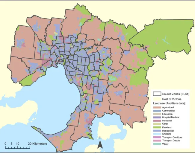
Figure 1: Map of the study area, showing Source zones (the SLAs) and the ancilliary data (land use classification) used in the study. ... 16
Figure 2: Schematic diagram of relevant nested Australian Bureau of Statistics data aggregations. ... 17
Figure 3: Graph showing the area occupied by the different land use classes within the study area, and the count of parcels of each land use type within the study area. ... 20
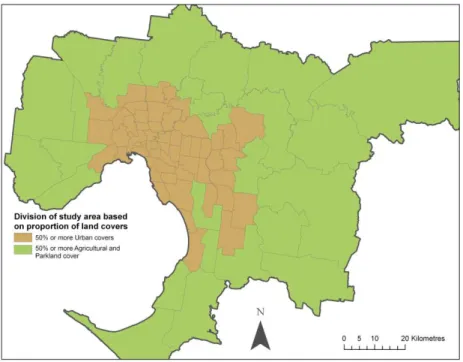
Figure 4: Division of study area based on the proportion of Urban or non-Urban (Agricultural and Parkland) covers. ... 25
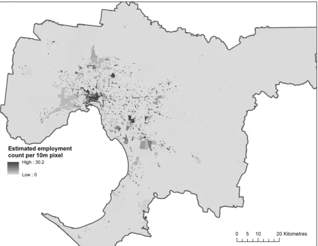
Figure 5: Best estimate of employment distribution, based on Poisson model with employment attributed to employment-related land uses. ... 35
Figure 6: Residual plots comparing the predicted values and residuals from the regression modeling stage to the predicted values and residuals from the employment estimate stage.
... 38
Figure 7: Residual count in Validation Zones from the employment estimate based on the Poisson employment land uses model. ... 43
Figure 8: Percentage error in Validation Zones from the employment estimate based on the Poisson employment land uses model... 44
Figure 9: Residual count in Validation Zones from the employment estimate based on the OLS all land uses model that was split by region... 45
Figure 10: Percentage error in Validation Zones from the employment estimate based on the OLS all land uses model that was split by region... 46
Figure 11: Residual plots comparing the predicted values and residuals from two working population estimates ... 48
Figure 12: Best estimate of working population distribution, using the density-weighted distribution method. ... 49
Figure 13: Residual count in Validation Zones from the working population estimate using the density-weighted distribution method. ... 50
Figure 14: Percentage error in Validation Zones from the working population estimate using the density-weighted distribution method.. ... 51
Figure 15: The 40 sites randomly selected for the employment containment study. They are overlaid on the best final employment estimate surface (based on the Poisson employment land uses model)... 52
LIST OF TABLES
Table 1: Land use classification derived from Australian Bureau of Statistics Mesh Block data, with notes about features... 19 Table 2: Results of Ordinary Least Squares regression models to determine relative
employment densities of land use classes. ... 34 Table 3: Results of Poisson regression models to determine relative employment
densities of land use classes. ... 34 Table 4: Comparison of error in the employment estimates ... 36 Table 5: Comparison of mean square error, etc. for the population estimates
produced by different models... 47 Table 6: Summary of employment and employment containment in selected
1.
INTRODUCTION
1.1
Rationale
This project studies employment containment in Melbourne, Australia.
Employment containment is a component of journey to work analysis, a rich field of
study relevant to contemporary transport planning, land use planning and labour market
analysis. Employment containment, in particular, is a measure of the proportion of people
that work in a location close to their home (studied by the likes of Burke, Li, & Dodson,
2010; Debenham, Stillwell, & Clarke, 2003; Yigitcanlar, Dodson, Gleeson, & Sipe,
2007). This measure is of interest because most urban planning academics and
practitioners have long advocated for land use planning strategies that emphasise a
mixture of housing and employment land uses. This approach, summarised by the term
‘Compact Development’ (Frank & Devine 2006) is thought to minimise a number of
economic externalities including commuting time and costs (Flood & Barbarto, 2005),
traffic congestion, and more recently, greenhouse gas emissions associated with climate
change (Burgess, 2000). When combined with other complementary strategies, a healthy
level of employment containment is thought to make a city a better place to live.
During at least the past decade, urban planning policies in Melbourne have been
driven by this Compact Development philosophy, and have aimed to improve local
employment opportunities and therefore employment containment in the city’s suburbs.
For example in 2009 the State Government of Victoria released their Melbourne@5
million planning strategy that was aimed at improving the environmental and social
sustainability of the city’s population growth trajectory over twenty years (Department of
Planning and Community Development, 2009). This policy explicitly outlined an aim to
change employment distribution in the city so that its resident population will have
greater access to employment closer to home, with the designation of targeted activity
transport and other infrastructure. The strategy was a reaffirmation of the Government’s
long term desire to move Melbourne from a ‘Monocentric’ to ‘Polycentric’ city so that
people have more opportunities to work and use necessary services closer to their homes.
With a political change of government at the end of 2010, this policy has since been
shelved in favour of a new Metropolitan strategy, still in development, which is almost
certain to be concerned with the same overarching urban planning issues. Therefore there
is still a clear need for ongoing empirical work in this area to underpin the development
of good public policy.
To assess the effectiveness and relevance of such urban planning policies now and
into the future, it is useful to understand the current journey to work and employment
containment patterns in Melbourne. While policies such as Melbourne@5 Million have
been developed with the assumption of a problem of inadequate employment
containment and an overconcentration of jobs in Melbourne’s Central Business District
(CBD), analyses of commuting patterns and employment containment in Melbourne's
suburbs are somewhat incomplete (Davies, 2010). Indeed, Davies points to the fact that
while there is a high concentration of professional jobs in the city’s CBD, around 90% of
the Melbourne metropolitan region’s jobs are located in the suburbs, suggesting that there
are already many jobs located close to people’s homes. Knowledge about who travels
where, however, is still underdeveloped.
Work commuting studies are made possible in Australia by Australian Bureau of
Statistics (ABS) data that records both the residential and work locations (where
applicable) of all people in Australia on the five-yearly census day. An
Origin-Destination matrix provides a summary of the number of people travelling from
residential locations to employment locations. Due to privacy restrictions, the matrix is
only made available in aggregated form, and most commuting and containment analysis
is conducted at the Statistical Local Area (SLA) level, an ABS designation (see for
Regional Economics, 2011), the larger municipal Local Government Area (LGA) level
(e.g Moriarty & Mees, 2006), or even at larger aggregations of these. Traditionally,
measures of containment are derived by counting the proportion of people who both live
and work within the same administrative or statistical boundary (Yigitcanlar, Dodson,
Gleeson, & Sipe, 2007). SLAs in the greater Metropolitan Melbourne area range in size
from 1.9 km2 in the CBD to 1137 km2 on the fringe of the metropolitan region, thus
comparisons of containment rates in SLAs are complicated by the varying size of the
areal unit. And while data detailing worker’s origin and destinations is available at
smaller ABS defined aggregations (namely Census Districts and Destination Zones),
analysts have appeared to shy away from using the data at this smaller scale because the
boundaries of these two data sources are not concurrent- thus the traditional containment
analysis method is not possible. At any rate, these smaller geographies are also not
uniform in size and shape and hence they still face the same problem of varying size as
do the SLAs.
While there has been some analysis of the rates at which people both live and
work within these broadly defined ‘local areas’, little work has been done to investigate
employment containment using smaller and more uniform catchment areas as the unit of
analysis. A finer scale analysis assisted by land use classification may provide the
opportunity for more meaningful employment containment comparisons, and provide a
greater understanding of which features of the urban landscape contribute to local
employment.
This thesis supposes that assessments of employment containment could be
assisted by interpolation or downscaling methods that have been widely used in the
general geographic literature. This could help to overcome the constraints of
area-aggregated data issued at the level of administrative or statistical boundaries. The rest of
this chapter reviews some relevant background and previous research in downscaling or
employment containment analysis, in order to formulate the thesis aims that appear at the
end of the chapter.
1.2
Related Work
1.2.1 Journey to Work and Employment Containment
Employment containment is one of a number of related employment metrics that
aims to describe the relationship between the working population’s place of residence and
place of work. Other related measures include job/housing balance, minimum commuting
distance or excess commuting (Boussauw, Derudder, & Witlox, 2011; Boussauw,
Neutens, & Witlox, 2010), and the number of accessible jobs. I consider employment
containment to be of particular interest because it is the metric that can tell us the most
about the current situation of employment localisation in Melbourne.
The traditional approach to employment containment is to calculate the proportion
of people living in an administrative or statistical boundary that also work within that
same administrative designation. This is a simple and quick indicator of the degree of
containment in a given area, but from a geographic analysis perspective it has some
limitations. The Modifiable Areal Unit Problem (MAUP) is often discussed when
analysing areal data (Páez & Scott, 2004), which is a generalisation of the Change of
Support Problem (COSP) (see the review of these topics by Gotway & Young, 2002).
These problems recognise that the changing size and shape of administrative boundaries
impacts on the rates at which a given phenomenon will be measured in those areas, and
hypothetically shifting those boundaries could lead to significantly different counts and
even an apparently different trend in the phenomena. It seems that this problem is
especially significant when dealing with the question of employment containment- after
all, the measure is traditionally based around the proportion of movement either within or
across administrative boundaries and so the position of the boundary or relative size of
boundaries would, by geography, seem more likely to contain workers within it compared
to another administrative boundary of a smaller size. Furthermore, one can imagine a
situation where people living close to the administrative boundary might travel a very
short distance across the administrative boundary for work, or a person living in the
extreme north of the administrative region travels to the southern extreme of the area
without passing the boundary. Within the traditional analysis of containment, the former
would be considered not to be contained while the latter would be, even though the
former had travelled a shorter distance.
When analysing commuting and employment containment some authors have
acknowledged this shortcoming in employing the traditional containment analysis
methods (Horner & Murray, 2002; Boussauw et al., 2011). Therefore such studies are
often taken to be only indicative and descriptive for a given area, rather allowing
meaningful comparison between different cities, or even different zones within a city.
Some authors have gone partway to overcoming the problem by aggregating up the
administrative regions until uniform rates of containment are reached within the
aggregations, thus creating ‘commuting regions’ that are controlled for containment rate
if not for physical size (eg Bill, Mitchell, & Watts, 2007; Watts, 2009; Johnson, 2010).
However, little work has yet been done in the opposite direction of disaggregating rather
than aggregating to overcome this problem (LeSage & Fischer, 2010).
At these broader scales, studies of 2006 ABS data have found that
self-containment rates in Melbourne are highest in the CBD (with a self-self-containment rate over
50%) and the larger SLAs in the outer reaches of Melbourne, which had containment
rates of 30-40% in most cases (Bureau of Infrastructure Transport and Regional
Economics, 2011). Some authors have looked at employment containment alongside
other socio-economic variables, for example a study of employment containment by
occupation that found that self-containment rates don’t vary greatly by occupation in
jobs are more likely to travel further for work, compared to people in low skilled
occupations (Bill et al., 2007).
Elsewhere in Australia, Yigitcanlar, Dodson, Gleeson, & Sipe (2007) used a road
network analysis between census collection districts to examine origin-destination work
flows in master-planned estates in Australia. This was a rare use of smaller areal units to
study employment containment, but the scope of the study was limited to a small number
of recently-developed suburbs that all exhibited low containment rates.
1.2.2 Areal interpolation
Areal interpolation is the process of inferring the data value of some phenomenon
in space where it has not been directly measured. The principles of areal interpolation are
useful where data has been collected and aggregated at one geographic resolution, but are
desired at a different resolution or aggregation. There are two related but distinct areal
interpolation problems- that of downscaling to sub-areal units, and spatial misalignment
of similarly sized by mismatched sets of administrative boundaries or other polygons (see
for example Lin, Cromley, & Zhang, 2011). Early attempts at areal interpolation were
later characterised as simple areal interpolation, using a uniform areal weighting to
assume that the target area for which some variable of interest is to be calculated will take
a proportion of that variable measured at the source area, proportionate to the fraction of
the source area that the target area occupies in space (Flowerdew & Green, 1992). A
variation on this areal weighting principle is Tobler’s pycnophylatic constraint method
(W. R. Tobler, 1979, and more recently employed by Kim & Yao, 2010 and Yoo,
Kyriakidis, & Tobler, 2010) which replaces the uniform distribution assumption of areal
weighting, with a smooth density function extending to adjacent source zones, while
retaining the original count of the source zones. Another, though less sophisticated
which collapses all the population data into a point and employs inverse distance
weighting.
1.2.3 Kriging and Geostatistics
Related to these smoothing techniques is the field of geostatistics, including
area-to-point kriging which smooths known rates of the phenomenon across space via
correlation of a variable with itself through space (e.g Kyriakidis, 2004). Geostatistical
methods produce error estimates that can indicate the accuracy of the interpolated surface
(Yoo et al., 2010). Smoothing may not be appropriate to the phenomenon under
investigation in this current study, since population and employment density are products
of their human-built urban environment, which can often have sharp edges and jumps in
values rather than smooth continuous surfaces. Intuitively this seems especially true for
measures of employment distribution as opposed to (residential) population distribution,
as nodes at which employment occurs tend to be much more clustered in the urban space,
compared to places at which residential population occurs, which tend to be more spread
out throughout the urban space. Therefore, kernel smoothing and area-to-point kriging,
with its focus on smoothing, do not seem to lend themselves to interpolating employment
density at a small scale. Further the underlying smoothness of the process must be
known or assumed. Nagle (2010) produced an employment surface via area-to-point
factorial kriging in order to study employment agglomerations in the Denver
metropolitan area. However, the scale of the interpolation was large and general, and no
ancillary data such as land use information was used to inform the kriging. Instead, a
standard covariance function was used. The main advantage of this method is the smooth
surface it produces, though in the case of the current study a smooth statistical surface is
not a high priority as employment density is not assumed to be a smoothly varying
1.2.4 Dasymetric methods
Following from the simple areal interpolation methods, intelligent methods were
developed that incorporate ancillary information about the likely distribution of a given
variable. These methods are often termed dasymetric and work in this field has tended to
focus on residential population as the variable to be interpolated (see for example
Mennis, 2003).
Dasymetric methods are characterised by their use of knowledge about the likely
distribution of some phenomena within a source zone. This additional knowledge is used
to distribute the known quantities of a given phenomenon at the source zones over the
study area, in order to infer quantities in target zones of a different scale or areal
aggregation. Dasymetric methods can be classed in a number of ways, with one of the
key distinctions being between binary and 3-class methods. In binary methods, the
variable in question is distributed evenly across areas that are thought to be occupied by
the phenomena, and not attributed at all to areas that are deemed to be unoccupied. In
three-class methods, the variable is allowed to have different densities or rates across the
occupied area, given knowledge or assumptions about the rates of that phenomenon in
different land classes. Many more recent studies have used this principle to downscale
population data based on land use or land cover, with population distributed at different
densities depending on known or assumed populations densities in different land use
classes (Langford, 2006; Mennis, 2003; Reibel & Agrawal, 2007). Mennis & Hultgren
(2006) termed these methods ‘intelligent’ and derived their own procedure where
analysts could use both sampling of population in various land cover classes, and their
own professional judgement to assign population density to various land cover classes.
This method, like most others variations of dasymetric methods, employed a
mass-preserving method in attributing population density, where the downscaled population
Various techniques have been used to derive the downscaled population
estimates. Ordinary Least Squares (OLS) (Langford, 2006; Yuan, Smith, & Limp, 1997),
Poisson (Flowerdew & Green, 1989), Bayesian (Mugglin, Carlin, & Gelfand, 2000) and
other regression methods have been used, where the coefficients derived in the regression
are treated as the relative population density of the various land cover classes. The
technique developed by Mennis and Hultgren (2006) relies on sampling population
densities from source zones that are entirely covered (or in some cases, mostly covered,
say by a threshold of 80% or more) by one of the land cover or land use classes of
interest. It can be noted here that while some authors distinguish between ‘dasymetric’
(binary or three-class sampling based methods) and statistical methods, Langford (2006)
writes that the various methods employed can be seen as variations along a continuum of
these two techniques. Indeed, density coefficients may be derived by global or regional
regressions, then re-scaled for each source zone to recreate the known population of that
zone (employing the mass-preservation constraint). In this way, the regression-derived
density coefficients act as ratios of the relative density that each land class should take.
Langford tested the binary dasymetric method against the various formulations of a
three-class dasymetric method. He found that combining regression with dasymetric re-scaling
of the density coefficients produced the most accurate results of the three-class methods;
however, within his case study a binary method actually performed better than all the
three-class methods, probably because it is less sensitive to fluctuations in different land
class densities.
Re-scaling is only one of the ways to ensure mass-preservation of the known
counts. Liu, Kyriakidis, & Goodchild (2008) provide a variation on the regression-based
dasymetric approach, by deriving population densities for each land use class via linear
regression, but then using area-to-point kriging to smoothly distribute the residual source
zone population counts to the target zones. Paralleling the sampling approach to
districts of entirely one land use zone in order to create the kriging semivariogram. The
advantage of using kriging for this process is that spatial information is incorporated to
attribute the population- e.g. if there is a high density population area in the vicinity then
this information is used to attribute the population, rather than attributing the population
uniformly. The authors of this study found that incorporating area-to-point kriging
reduced Root Mean Square Error (RMSE) compared to the regression alone. Similarly,
Kim & Yao (2010) combined dasymetric methods with pycnophylactic smoothing,
created a smoothed population surface that was superior to either a standard dasymetric
or standard pycnophylatic interpolation.
Whichever method is used, the effectiveness of intelligent dasymetric methods
relies most heavily on the usefulness of the ancillary data for modelling the particular
phenomenon in question. Gallego (2010) compared a number of dasymetric variations:
the Expectation-Maximisation Algorithm, based on Dempster, Laird, & and Rubin
(1977); logit regression; and the Limiting Variable method (based on Eicher and Brewer,
2001), which attributes a minimum population density to all classes in the study area,
then distributes the remainder across other classes, assigning particular density thresholds
along the way. Gallego found that the choice of algorithm did not have a great impact on
the accuracy of the downscaling. Langford (2006) also emphasised the point that the
ancillary data are of greatest importance. A variety of ancillary supports can potentially
be employed, such as land cover or land use classes (Gallego, 2010), remotely sensed
images (Deng, Wu, & Wang, 2010; Harvey, 2002; Silván-Cárdenas et al., 2010), road
network data (Li et al. 2010) attributing population to areas where road network is
present, cadastral boundaries (Maantay & Maroko, 2009) and address point data
(Zandbergen, 2011).
In either the sampling or regression based methods, the classical approach
assumes that relative population densities are stationary across the study area. However,
in different relative population densities across the different land classes present. Some
analysts have attempted to account for geographic non-stationarity of population density
across the study area. Mennis (2003) sampled population densities from sub-units within
each county to derive local densities, in order to account for differences in the
urbanisation of different counties. Langford (2006) found that using regional (at UK
District level) rather than global regressions produced a more accurate prediction, as long
as enough units were available within regions to perform a reliable regression. However,
Langford rightly pointed out that using District or any other such boundary as a basis for
forming regions is quite arbitrary, and therefore may not be representative of density
variations across space. Lin et al. (2011) approached this problem by using
geographically weighted regression (GWR) to derive population densities. While noting
that the GWR was more successful in spatial misalignment problems than downscaling
problems, overall they concluded that for their study area GWR did a better job of
interpolating than OLS regression did. Another form of weighted regression, Quantile
Regression, was recently used to perform areal interpolation of population (Cromley,
Hanink & Bentley, 2011). Although it is not specifically a form of spatial regression,
quantile regression can be used to derive a regression line and therefore unique regression
coefficients for each observation (i.e., source zone) in a study area. The authors of this
study also found that this method outperformed OLS regressions and binary dasymetric
methods.
Brinegar & Popick (2010) recently compared a number of different population
estimation methods, including land-use based 3-class dasymetric methods, road
network-based dasymetric methods and statistical regression. Their comparison and discussion
points out that different methods have differing strengths and weaknesses in estimating a
population based on different conditions, such as heterogeneous land use and unusually
high or unusually low population density. This highlights the lesson that a particular
produce the best result under other conditions. This raises an important distinction for the
current study. This review of the dasymetric literature has mainly focused on
downscaling population data. The bulk of the dasymetric literature focuses on this
problem, rather than downscaling other socio-economic variables (such as employment
distribution as in this study). Since employment has a different spatial distribution to
residential population, findings from this literature may not translate easily to the
downscaling of employment data.
One related problem that has attained some attention, however, is inferring
daytime as opposed to nighttime population distribution. In general, population data
record a person’s residential address. Most people spend evenings and nights at their
residential address, but much fewer are there during the day- they are either at work,
school, or involved in other activities. Researchers interested in emergency management
and traffic planning, for example, are more interested in daytime than nighttime
populations. For example Sleeter and Wood (2006) used dasymetric techniques based on
a detailed business database, and Kobayashi, Medina, & Cova (2011) used the
pycnophylactic method to produce a smooth population surfaces that was appealing and
easy for policy makers to look at and understand, and displayed expected population
distribution at different times of the day. This work is similar to the interests of the
current study, though the purpose for looking at the daytime population may be different.
1.2.5 Areal interpolation and journey to work
Use of areal interpolation methods alongside commuting analysis is so far limited.
Li, Corcoran, & Burke (2010) used areal interpolation to paint a more detailed picture of
the origin-destination work flows at a sub-areal scale, using the road network to perform
binary dasymetric downscaling of commuting flows in South East Queensland. In another
example, Boussauw, Neutens, & Witlox (2010) produced a 4 km grid interpolated surface
Jang & Yao (2011) produced an interpolation using ‘flow lines’ of an
origin-destination matrix of traffic flow data, focusing on aligning mismatched traffic zone and
census zone data sources, rather than downscaling the origin-destination flows. In this
case, no ancillary data was employed to support the interpolation. Kaiser & Kanevski
(2010) produced a dasymetric population mapping method explicitly to assist with traffic
modelling, focusing on residential population.
1.3
Formulation of this study
The aim of this study is to explore a process for estimating employment
containment in uniform catchment zones around a given employment centre. In
particular, the key questions posed by this study are:
1. Can dasymetric processes (binary, sampling and regression approaches) assist in
producing a useful employment containment measure that overcomes some of the
spatial irregularity problems associated with traditional employment containment
measures?
2. What do these derived measures say about employment containment in the study
area of Melbourne, Australia?
In order to achieve this, a downscaled estimate of both employment and working
population distribution is required. In particular, binary dasymetric and 3-class methods
are explored for deriving these distribution estimates. A workflow is developed that
includes a validation step to give an indication of the accuracy of the derived employment
and population surfaces.
From the final employment surface, a number of employment centres are
randomly selected and an employment containment catchment is derived from a 5 km2
commuting distance catchment. Commuting flows from an origin-destination matrix are
areally weighted to estimate flows into the employment centres from the 5 km2
A brief analysis of the employment containment of these centres is presented, as
well as an assessment of the performance of the downscaling process for enabling a
2.
DATA AND METHODS
There are three parts to the analysis: Estimating employment distribution,
estimating working population (residential) distribution, and then combining these for the
employment containment estimate in fixed catchments around selected employment
centres. A description of this process follows the details of the study area and the data
used. The R statistical program was used to perform the regressions, ArcGIS analysis
tools are primarily used to perform GIS tasks and Excel 2010 was used for data
manipulation.
2.1
Study Area
The focus of this study is the greater metropolitan region of Melbourne, Australia
(see Figure 1). At the time of the 2006 Census (from which all data for this study is
sourced), the total population of the greater Metropolitan region was 3 599 644 people.
There were 1 741 193 people living in Melbourne and adjacent regions (the population of
focus in this study) who were employed (termed ‘working population’ from hereon).
Furthermore, 1 507 060 people identified their workplace as within one of Melbourne’s
Destination Zones (as described further below).
2.2
Data
Following the formulation of Gregory (2002), Langford (2006) and Li and
Corcoran (2010), the data used to perform the employment and working population
downscaling in this study is designated at four nested levels, shown in Figure 2 and
outlined in the text below. All data is derived from the Australian Bureau of Statistics
Figure 1: Map of the study area, showing source zones (the SLAs) and the ancillary data (land use classification) used in the study.
2.2.1 Source zones
Source zones are administrative boundaries with counts of either the number of
people working in that zone (for the employment surface downscaling) or the number of
employed people that live in that zone (for the working population downscaling). These
are the known counts from which the downscaled estimates will be derived. In this study,
the ABS SLA designation is used as the source zone in both the employment and
working population downscaling. In the Melbourne study area there are 80 SLAs, which
Figure 2: Schematic diagram of relevant nested Australian Bureau of Statistics data aggregations.
2.2.2 Target zones
Target zones are the unit at which the downscaled data is estimated. The zone
may be another administrative designation for which the count data of interest is not
available, some other user-defined designation, or a uniform raster surface. In this study
the latter is chosen, at a 10m resolution, as this can more easily be integrated with the
employment catchment study in which it will be deployed.
2.2.3 Ancillary data
Ancillary data supports the downscaling by providing information about how the
variable of interest is distributed in the source zones (and therefore how it should be
attributed to the target zones). Where dasymetric downscaling has been performed on
population counts (by far the most common variable studied in the dasymetric literature),
the ancillary data is usually in the form of land cover categories or remotely sensed
imagery that may be used to categorise urban areas into residential density classes.
However, little work has been done to perform downscaled employment estimates via
these methods, and intuitively one suspects that estimating employment either by land
(as opposed to land cover) classification is available from the ABS, in the form of Mesh
Blocks.
Mesh Blocks are the smallest designation at which ABS population data are
available at, and includes a population count and a land use classification for each area.
The land classes are relevant for determining employment and non-employment land
uses. The land use classification is described in detail in Table 1, and their distribution
with the study area is displayed in Figure 1. This classification is used as the basis for
redistributing the employment and working population counts, and the population count
is also used in the working population estimate. Note that in the original ABS
classification the classes ‘Transport Depots’ and ‘Transport Corridors’ are a single class
called ‘Transport’. They are split for the purposes of this study because they clearly
represent different land uses. There are 47 725 Mesh Blocks in the study area. The
distribution of the Mesh Block classes amongst the different classes, and the total area
Table 1: Land use classification derived from Australian Bureau of Statistics Mesh Block data, with notes about features
Land class Description Number
of parcels
Total area (km2)
Commercial Business and shopping zones, office blocks, strip shopping zones, shopping malls
1800 92.4
Education Schools (primary and secondary), university campuses 1262 56.4
Industrial Manufacturing, warehousing 814 251.4
Hospital/Medical Hospitals or other large medical centres 78 3.9
Shipping Mostly offshore regions designated as shipping zones 2 0.7
Residential Areas primarily occupied by housing 37259 1676.2
Agricultural Farming land 836 5190.3
Parkland Regional and local parks of varying size 5082 5220.3
Other Miscellaneous land uses such as water treatment plants and military accommodation
23 16.7
Transport Corridors Land along railway lines 438 14.6
Transport Depots Minor suburban airfields, public transport depots 5 8.2
20
Figure
3
: Graph showing the area occupied by the different land use classes within the
study area (top), and the count of parcels of each land use type within the
study area (bottom).
0
10000 20000 30000 40000
Agricultural
Commercial
Education
Hospital/Medical
Industrial
Other
Parkland
Residential
Shipping
Transport Corridors
Transport Depots
0
2000 4000 6000
Agricultural
Commercial
Education
Hospital/Medical
Industrial
Other
Parkland
Residential
Shipping
Transport Corridors
Transport Depots
2.2.4 Validation zones
Validation zones are used to re-aggregate the downscaled data to test how
accurately the downscaling process distributed the variable in question. Since ABS data
aggregations are for the most part nested as smaller and smaller aggregations that can be
aggregated up to a larger designation (e.g, Mesh Blocks can be combined until they are
coincident with the SLA boundary), the known employment or working population
counts at a designation smaller than the source zone must be used to validate the
employment and working population estimates. The SLAs are further subdivided into
Destination Zones associated with employment counts, and Origin Zones associated with
residential counts. Origin Zones and Destination Zones are of similar size but generally
have misaligned boundaries. In this study I use an aggregation that the Victorian
Department of Planning and Community Development specifically developed for
studying work and home locations of commuters- therefore the geography is different and
slightly more coarse than that normally available from the ABS. There are 1301 Origin
Zones and 652 Destination Zones in the geography used in this study.
2.2.5 Transport Network
To produce the commuting catchments around employment centres as part of the
employment containment estimate, I use a vector layer of the Major Roads and Railway
lines of Melbourne.
2.2.6 Commuting Data
To produce the employment containment estimate, information about the
employment distribution must be linked to information about the working population
distribution. An Origin-Destination matrix tallies the number of people residing in an
2.3
Downscaling employment data
The literature on areal interpolation provides a number of variations on the
process of downscaling. Dasymetric approaches can roughly be divided into
based approaches and regression-based approaches (Langford, 2006). The
sampling-based method was discussed by Mennis (2003). The method relies on sampling the
population (or in this case, employment) density of the various land classes from zones
that are entirely covered or close to entirely covered (80% or more) by one land class.
This is in order to derive an average employment density for that land class. Where the
study area size allows it, Mennis recommends dividing the study area into sub-regions,
such as municipalities, to better account for spatial differences in the variable of interest.
Early data analysis for this study indicated that the SLAs are too large to provide sample
zones that are covered or even 80% covered by each land class. Li & Corcoran (2010)
had a similar finding when using dasymetric methods to perform downscaling based on
SLAs in a South East Queensland study area. The authors instead use a regression
method.
2.3.1 Regression-based approach to deriving employment
densities
A number of authors use linear regression to produce relative population densities
of classes within their study area. OLS regression, which minimises the sum of squares of
the residuals, is commonly used in this context including by Harvey (2002), Langford
(2006), Reibel & Agrawal (2007), Yuan et al., (1997), and Li & Corcoran (2010). Under
this model, the variable of interest E (employment distribution) at the source zone is
equal to the sum of the variable’s density of each class C multiplied by the area A of that
𝐸𝐸=𝛼𝛼+ 𝛽𝛽
𝐴𝐴 + 𝜀𝜀
Therefore, given that E and A are known, the density in the land class equates to
the regression coefficient and can be derived from the OLS regression. The coefficient
corresponds to a global relative population density of each land class. In this case, the
employment count for each SLA is regressed against the amount of each land use class in
that SLA. A number of different configurations are tested in order to find a best fitting
model.
An alternative to the OLS regression is Poisson regression. A Poisson distribution
is often considered to be the best model for population counts (Flowerdew & Green,
1989, 1992), and a Poisson regression helps to avoid producing negative population totals
in the final estimate (Langford, 2006). However a Poisson model has the assumption that
the conditional variance of the outcome variable equals the conditional mean.
Regardless of whether OLS or Poisson regression is used, a regression without an
intercept is recommended, since a theoretical source zone with zero area should have a
zero employment count (Langford, 2006; Yuan et al., 1997; Harvey, 2002). In this study I
test both OLS and Poisson regression models to compare their accuracy in describing
relative employment densities in the study area.
A number of variations on the models are tested, altering the variables in the
model to find the most fitting descriptors of employment distribution. These variations
seek to distribute employment amongst the land classes in a way that best mimics the
known distribution of employment in the source and validation zones. Should the model
include information about all the land classes present in the source zone, or should it only
classes; from here on referred to as ‘Employment land uses’)? Or perhaps something
between the two, excluding only land classes that are clearly not associated with
employment (Parkland, Water, Shipping, and Transport corridors), while including some
that might support some employment (Residential, Transport depots, ‘Other’, these along
with the Employment land uses are from here on referred to as ‘Urban land uses’). These
variations are run in different versions of the model.
Local regressions that break the study area into some smaller regions for analysis
have been used successfully in some cases (Langford, 2006; Yuan et al., 1997). As
discussed by Langford (2006), using local regression raises the question of precisely how
to break up the study area into ‘local’ areas and demands that the local areas have enough
sub-areas for a robust statistical sample. Using a larger administrative designation is a
commonly suggested solution, but is quite an arbitrary way to divide the study area, and
at any rate in the context of this study there is no obvious administrative designation that
could break the study area into smaller regions. An alternative is to break the study area
into regions based on the relative representation of land use classes in the source zones.
The Melbourne study area has a concentric form where the inner urban/suburban core,
covered by relatively small SLAs dominated by urban covers, is surrounded by a ring of
larger SLAs characterized by lower overall urban cover and a high proportion of
agricultural land or parkland (Figure 4). Since the global density estimates derived by the
regressions in fact represent the relative employment densities that each land use class
should take, it is possible that globally derived employment densities may not adequately
describe these differing forms. Therefore the study area is split into two regions, one
where the Agricultural and Parkland classes represent 50% or more of the land in the
source zone, and the other where all the other classes represent 50% or more of the
source zone.
A final variation is introduced in an attempt to control for the difference in the
source zone is regressed against the fraction of the source zone that each land class
represents. In this case the coefficient derived is a density fraction.
To assess the suitability of the resulting regression model, a number of statistics
are used. The R2 value is a measure between 0 and 1 of how well the model describes the
Figure 4: Division of study area based on the proportion of Urban or non-Urban (Agricultural and Parkland) covers.
regressed data, with values closer to 1 indicating better fitting models. While there is
some controversy around best way to measure model fit for OLS regressions with no
intercept, Eisenhauer (2003) notes that the R2 value is valid as long as it is used to
compare no-intercept models to each other.
Aikake’s Information Criterion (AIC) can also be used to compare model fit.
Models with a smaller AIC score are considered to be better models because the score
penalizes models that have a large number of explanatory variables (Rosenhein, Scott, &
indicator of the model fit (Rosenhein, Scott, & Pratt, 2011). These three measures are
used as a general indicator of model fit to select the best fitting models that are then
tested by generating employment estimates based on the regression coefficients.
The detailed R script of the regression modelling is shown in Appendix A.
2.3.2 Generating employment estimates
There are two possible approaches for producing the downscaled employment
surface: assigning the downscaled population to the areas that were used as classified
ancillary data, or creating a raster surface. Liu et al. (2008) argue that a surface is the
preferred output, as this is easier to integrate with other data sources. Therefore in order
to generate the population estimates, I first produce a 10m-resolution raster with the
values in the raster being the regression-derived density coefficients for the relevant land
use class at that location (multiplied by a factor of 100 to equal the density of a 10m2
raster cell).
Applying the regression derived density coefficients to the study area results in
over and underestimation of counts at the source zone level (literally the residuals of the
regression performed to derive the density coefficients). There are at least three ways that
these residuals are dealt with in the literature: 1) not at all; 2) by using area-to-point
kriging to smooth the residual across the source zone (Liu et al., 2008); and 3) re-scaling
the global density estimates within each source zone so that they reproduce the known
count within the zone, a condition known as mass preservation or the pycnophylactic
constraint (W. R. Tobler, 1979). Option 1) is disregarded as unsuitable for the current
study; Option 2) is investigated but requires sampling of employment density in source
zones of entirely one land use zone in order to create the kriging semivariogram. As was
discussed in the introduction to this section in relation to employing the sampling-based
allow such sampling. Option 3) is therefore adopted as it is both possible and easy to
apply in the context of this study.
To apply the re-scaling, the initial estimate in each source zone is summed using
the Zonal Statistics tool in ArcGIS, and a re-scaling factor for each land class within each
source zone is derived by the following equation (Gregory, 2002; Langford, 2006):
𝑑𝑑 =𝐸𝐸𝐸𝐸
∙𝑑𝑑
Where dcs is the density estimate for land class c in source zone s, Es is the actual
employment count in the source zone, Eis is the estimated employment count in the
source zone produced by the initial global density estimate, and dc is the initial global
density estimate in class c. The new locally-scaled densities are then applied to the study
area using a Raster Calculator operation, multiplying the rescaling factor by the original
global densities as in the above equation. This derives a final fine-scaled employment
estimate for each 10m2 cell in the target raster.
In addition to the regression-based estimates, a binary estimate of employment
distribution is produced, following the method discussed in Langford (2006) and Mennis
(2003). This is a simplified version of the above process, where employment land uses
are given a raster value of ‘1’, and non-employment land uses a value of ‘0’. Zonal
statistics are summed to find the area of employment-occupied land in the source zone.
The employment count is divided by the employment-occupied area to derive an
employment density for the source zone. The employment density for each source zone is
then applied to the employment-occupied area via the Raster Calculator, producing a
final binary estimate of employment distribution with an equal employment density for
all employment land covers in each source zone.
Destination Zones). I compare a number of measures of the residuals of the estimate.
The RMSE as is calculated, and the Adjusted RMSE which follows Gregory, (2002) and
Lin et al. (2011), adjusting the RMSE to take account of the original observed population.
These are measures of the average variance of the estimate compared to the known
employment counts in each validation zone, and thus the accuracy of the downscaled
estimate. A similar measure is the coefficient of variation following Fisher & Langford
(1995), which divides the RMSE by the mean of the source zone populations. The Mean
Error is the average of the difference between the estimated and observed employment
count values. Note that given the mass-preserving constraint applied during the
downscaling process, where the initial estimate was re-scaled to match the known
employment counts in the source zone, the Mean Error should theoretically always be
zero. However, some error is added when translating values between the areal-based
employment counts or estimates, and the density values stored in raster form. Therefore
the Mean Error can be seen as a measure of the error arising from reaggregating raster
values to an areal-based count at the validation zones.
The abovementioned metrics are compared for each of the five employment
distribution estimates to identify the most accurate estimate. A detailed script of the
regression-based employment estimate procedure is given in Appendix B; the script for
the binary estimate is given in Appendix C.
2.4
Downscaling working population data
For the working population estimate, the study area is expanded to include Source
zones adjacent to Melbourne, in order to include any working population that may be
within a 5 km commuting distance of employment centres in the Melbourne study area.
Two estimates of the residential working population are produced. The first is a binary
employment estimate. However, for the working population estimate, the residential land
class takes the value ‘1’ and all other classes take ‘0’.
The second estimate is weighted by the known total population density of each
Mesh Block zone. A raster surface is produced of the known total population density of
the study area, again at 10m resolution. Zonal Statistics in ArcGIS is used to calculate the
total population of the source zone. Then, the known working population of the source
zone is divided by the total population of the source zone, to derive a working population
weighting for each source zone. The total population raster is multiplied by the working
population weighting in the Raster Calculator, to derive the final working population
estimate.
Once again the RMSE, Adjusted-RMSE, Coefficient of Variation and Mean Error
are used to assess the accuracy of the estimates once re-aggregated to the validation
zones. A detailed script of the working population estimate procedures are given in
Appendices C and D.
2.5
Employment containment assessment
In order to make an estimate of employment containment, the employment and
working population distribution estimates need to be linked to the known flows of people
from the Origin Zones to a destination SLA; and then, these flows must be downscaled
accordingly. The flows are stored as an origin-destination matrix. The matrix is imported
to ArcGIS with the destinations represented by individual records and the origins
represented by database fields.
From the best estimate of employment distribution, the final employment raster
dataset is converted to a polygon feature class. A subset of 40 ‘employment centres’ (any
parcels that are estimated to have some employment associated with them) is selected to
perform the containment assessment. The subset is randomly selected from those
accuracy. The random selection was performed using the ‘Sampler’ toolbox in ArcGIS
(Harold, 2011). The centres were visually inspected on Google Maps to identify their
location within the local urban landscape, and the classification of the land use was
identified from the Mesh Block data.
To generate the 5km2 commuting distance catchment around each employment
centre, the centroids of each of these parcels was first derived. The centroid point is used
to represent the employment centre as part of a Service Area Analysis, a feature of the
Network Analyst extension in ArcGIS. Line coverage of the major road and railway for
Melbourne is included in the analysis to create the 5km2 commuting catchments around
each of the centres. While theoretically a number of different distances could be chosen
for the study, 5km is chosen in order to investigate rates of highly localised employment.
Travel surveys from the Victorian government suggest that about 35% workers travel less
than 10 km to work each day, while around 15% travel 5 kms or less (Bureau of
Infrastructure Transport and Regional Economics, 2011).
A number of spatial intersections and table joins were performed to derive the
employment containment estimate. The aim is to calculate the number of workers in this
catchment that work in the employment centre, as well as the total working population of
the catchment in order to calculate a percentage of containment.
Each catchment polygon was associated with the employment centre point so that
information about the location of the employment centre and the employment estimate
was retained. The catchment polygons were intersected with Origin Zones (the working
population validation zones) to identify the part of these zones that fall inside the
employment catchment. Running Zonal Statistics calculates the estimated working
population in each of the Origin-catchment intersection zones. This is related to the
estimated working population in the entire Origin Zone (calculated during the validation
step of the working population estimate). The proportion of the working population of the
The data is spatially joined with the employment source zones (the SLAs) so that
the proportion of the source zone’s employment that occurs in the employment centre,
can be calculated.
To estimate the number of workers from the catchment that work in the
employment centre, the following equation is used:
𝐸𝐸 = 𝐸𝐸𝐸𝐸
×𝐸𝐸× 𝑃𝑃
𝑃𝑃
Where El is the number of people from the local catchment area working in the
employment centre, Et is the employment estimate for the employment centre, Es is the
known employment count from the source zone, and Eso is the count of people working in
the source zone that travelled from origin o. Poc is the estimated working population
living in the part of the Origin Zone covered by the employment catchment, and Po is the
estimated total working population of the Origin Zone. The contribution of each Origin
Zone in the catchment area is summed to reach El. The calculations were performed in
Excel. The Employment containment of the employment centre is calculated as the
proportion of the working population in the catchment, that works in the employment
centre. Additionally, the percentage of people working in the employment centre that
3.
RESULTS
3.1
Deriving employment density from regressions
During the analysis it became apparent that the one SLA covering the CBD of
Melbourne could be considered an outlier as it has the highest employment count but the
smallest overall area. Therefore models were run excluding this outlier from the analysis.
It is difficult to compare the Poisson and OLS models as an R2 score is not
produced for the Poisson models. Therefore, the Poisson and OLS models are considered
separately. The results of the various OLS models are shown in Table 2. A simple
ranking for the OLS models was produced by ranking all the models by their R2 score,
with the highest R2 ranked as 1, second highest as 2, and so on. The models were then
ranked again by AIC score, with the lowest AIC ranked as 1, and so on. The two ranks
were then summed and the models ordered lowest to highest based on this score, to find
the best fitting model.
The model that covered the agriculture-and-parkland dominated region only was
the best fitting model. This does not necessarily tell us anything special as the high R2
and low AIC may be a direct result of the small sample size of this regression compared
to the other regressions (Langford, 2006): There were 26 source zones for the
agricultural-parkland-dominated region and 53 source zones for the urban-dominated
region, compared to 79 source zones for the whole study area.
Of the models covering the whole study area, the model with all land uses and
using density fractions appears to have the best fit, followed by the employment model
that used density fractions.
The OLS models of the whole study area that used the raw data were the lowest
ranking of the OLS models. In general, however, these produce a significant estimate of
the density coefficients of the various land covers, where other better-ranking models did
The results of the Poisson models is shown in Table 3. For the Poisson models, no
R2 score is generated for the models, so the Poisson models are compared and ranked
based on their AIC score only. Additionally, as density fractions cannot be used in the
Poisson model (as the Poisson model is designed specifically for count data), there is a
smaller number of Poisson models than OLS models.
Of the Poisson models, the model with the full land covers was the best fitting,
followed by the urban model and the employment model. All the Poisson models tested
were found to produce significant estimates for all the land use classes included in that
model.
It is difficult to select which are clearly the best fitting regression models, as there
is inconclusive information provided by the two or three tests applied. In any case, these
regression models only produce a preliminary density estimate that will be scaled during
process of producing the employment estimates. Therefore I decided to generate
employment estimates from all of the models, rather than eliminate possible best fitting
models at this stage.
3.2
Producing employment estimates
A summary of the accuracy of the employment estimates produced by the various
models is shown in Table 4. Comparing the various fit metrics produces the unexpected
finding that the Poisson model with employment land classes and covering the entire
study area produced the employment estimate with the lowest overall error, despite being
one of the poorest fitting models based on the initial regression. Conversely, the estimate
that incorporated different densities for the urban-dominated and
agricultural-and-parkland-dominated regions produced more error than the estimate based on a universal
model, even though the results of the initial regression models suggest that these were the
34 Table 2: Results of Ordinary Least Squares regression models to determine relative employment densities of land use classes.
Co=Commercial, Ed=Education, In=Industrial, Ot=Other, Sh=Shipping, HM=Hospital/Medical, Re=Residential, TD=Transport Depot
Model R2 AIC Significant estimates R2
ranking AIC ranking
Overall score
All land covers, Agriculture/park dominated region, raw data 0.971 495.3 Co, In, Ot, Sh 1 1 2
All land covers, All study area, density fraction 0.915 982.5 Co 2 4 6
Employment land covers, All study area, density fraction 0.878 720.2 Co, Ed 4 3 7
All land covers, Urban dominated region, raw data 0.900 1135.0 Co, HM 3 5 8
Urban land covers, All study area, raw data 0.876 1667.9 Co, HM, In, TD 6 2 8
All land covers, All study area, raw data 0.877 1672.7 Co, HM, TD 5 8 13
Urban land covers, All study area, density fraction 0.721 576.1 Co, In, Re 8 6 14
Employment land covers, All study areas, raw data 0.862 1669.9 Co, Ed, HM, In 7 7 14
Table 3: Results of Poisson regression models to determine relative employment densities of land use classes.
Model AIC Significant estimates Ranking
All land covers, All study area, raw data 7650406 All 1
Urban land covers, All study area, raw data 8465964 All 2
employment estimates than the OLS models. The best employment estimate is displayed
on a map in Figure 5.
Table 4: Comparison of error in the employment estimates
Model name RMSE Adjusted RMSE Coefficient of Variation Mean Error
Poisson, employment land uses, all study area, raw data
2060.6 1.55 0.90 -0.00009
Poisson, urban land uses, all study area, raw data 2164.6 2.04 0.94 -0.00002
Poisson, all land uses, all study area, raw data 2332.8 2.41 1.02 -0.012
OLS, all land uses, all study area, raw data 2489.0 1.93 1.08 -0.001
Binary estimate, employment land uses 2531.4 3.42 1.10 -0.000004
OLS, employment land uses, all study area, raw data
2625.9 3.68 1.14 -0.00003
OLS, all land uses, regions split, raw data 2633.7 3.41 1.15 58.1
OLS, urban land uses, all study area, raw data 2694.5 2.36 1.17 -0.00007
OLS, all land uses, all study area, density fraction
10193.5 8.04 4.44 -0.09
OLS, urban land uses, all study area, density fraction
11062.6 8.15 4.82 -0.0001
OLS employment land uses, all study area, density fraction
15596.7 10.09 6.79 0.0002
Figure 6 shows residual plots for each model tested, comparing the predicted
values and residuals from the regression modelling stage (left) to the predicted values and
residuals from the employment estimate stage (right). Note that that since the predictions
at the modelling stage are based on source zones while the predictions at the employment
estimate stage are based on validation zones, the number of predictions and their scale are
different between each pair of plots. Examining these plots helps to understand the
models and how the error (residual) in the estimates changes between the model stage
and the employment estimate stage (where the estimated densities are rescaled to fit the