www.scielo.br/rbg
GEOTHERMAL GRADIENT AND HEAT FLOW IN THE STATE OF RIO DE JANEIRO
Antonio Jorge de Lima Gomes
1and Valiya Mannathal Hamza
2Recebido em 31 marc¸o, 2005 / Aceito em 12 dezembro, 2005 Received on March 31, 2005 / Accepted on December 12, 2005
ABSTRACT.Results of geothermal studies carried out at 72 localities have been used in evaluation of temperature gradient and heat flow values of the upper crust in the state of Rio de Janeiro. The investigations included temperature logs in boreholes and wells, calculation of geothermal gradients, measurements of thermal conductivity and determination of heat flow density. In addition, estimates of temperature gradients and heat flow were also made for areas of thermo-mineral springs, based on the so-called geochemical methods. Analysis of these data sets, after incorporation of appropriate corrections (for the perturbing effects of drilling operations, topography and climate changes) has allowed for the first time a better understanding of the regional distribution of thermal gradients and heat flow within the study area. The results obtained indicate that geothermal gradient values are in the ranges of 14 to26◦C/km in Precambrian metamorphic terrain and 19 to33◦C/km in areas of Phanerozoic sedimentary basins. Most of the rock formations are characterized by thermal conductivity values varying from 2.2 to 3.6 Wm-1K-1. Consequently regionally averaged mean heat flow values are found to fall in the interval of 40 to 70 mW/m2. Computer generated contour maps reveal that geothermal gradients and heat flow are systematically high in the western compared to the eastern parts of the state of Rio de Janeiro. There are indications that this geothermal anomaly is probably associated with the belt of Tertiary alkaline intrusives, between Itatiaia and Cabo Frio. Residual heat of large scale magma intrusions in the later part of the Tertiary period may be one of the possible mechanisms responsible for this thermal anomaly.
Keywords: Geothermal Gradient, Heat Flow, Rio de Janeiro.
RESUMO.Resultados de estudos geot´ermicos efetuados em 72 localidades foram utilizados na avaliac¸˜ao de gradientes de temperatura e o fluxo geot´ermico da crosta superior no Estado do Rio de Janeiro. As investigac¸˜oes inclu´ıram a realizac¸˜ao de perfilagens t´ermicas em furos e poc¸os, determinac¸˜ao dos gradientes t´ermicos, medic¸˜oes de condutividades t´ermicas e estimativas da densidade do fluxo geot´ermico. Como complementos, tamb´em foram estimados gradientes e fluxo geot´ermico das ´areas de ocorrˆencias de fontes termo-minerais, utilizando m´etodos geoqu´ımicos. An´alises desses dados ap´os a incorporac¸˜ao das correc¸˜oes apropriadas (efeitos de perfurac¸˜ao, topografia e variac¸˜oes clim´aticas recentes) tornaram poss´ıvel pela primeira vez um melhor entendimento da distribuic¸˜ao regional de gradientes t´ermicos e do fluxo de calor na ´area de estudo. Os resultados obtidos indicam que os gradientes t´ermicos variam entre 14 e26◦C/km nas regi˜oes metam´orficas Pr´e-Cambrianas e de 19 a 33◦C/km nas ´areas de bacias sedimentares Faneroz´oicas. Muitas das formac¸˜oes rochosas apresentaram condutividade t´ermica compreendida entre 2,2 e 3,6 Wm-1K-1. Conseq¨uentemente, os valores m´edios encontrados para o fluxo geot´ermico regional situam-se no intervalo de 40 a 70 mW/m2. Mapas de contorno, preparado a fim de examinar as variac¸˜oes regionais, revelam que o gradiente e o fluxo t´ermico s˜ao sistematicamente mais elevados na parte oeste da ´area de estudo, em comparac¸˜ao com aquelas encontradas na parte leste. Existem indicac¸˜oes de que a anomalia geot´ermica na parte oeste est´a provavelmente associada com a faixa das intrusivas alcalinas Terci´arias situadas entre a regi˜ao de Itatiaia e Cabo Frio. O calor residual das intrus˜oes magm´atico do per´ıodo Terci´ario superior configura-se como um dos poss´ıveis mecanismos respons´aveis por esta anomalia t´ermica.
Palavras-chave: Gradiente T´ermico, Fluxo Geot´ermico, Rio de Janeiro.
1Laborat´orio de Geotermia, Observat´orio Nacional – MCT, R. Gal. Jos´e Cristino, 77 – S˜ao Crist´ov˜ao, 20921-400 Rio de Janeiro, RJ, Brasil. Tel: 55 21 3878-9154; Fax: 55 21 2580-7081 – E-mail: [email protected]
INTRODUCTION
We report in the present work results of experimental determina-tions of geothermal gradients and heat flow carried out during the period of 1998 to 2001, in the state of Rio de Janeiro and adja-cent areas. The history of geothermal studies in this segment of southeastern Brazil is relatively recent. Systematic investigations began during the second half of the decade of 1990, soon after the installation of the Geothermal Laboratory at the National Ob-servatory (Observat´orio Nacional – ON/MCT). Prior to this period the only heat flow values reported for the state of Rio de Janeiro were estimates based on geochemical methods by Hamza & Es-ton (1981) and Hurter et al. (1983). Lack of direct experimental determination of geothermal gradients and heat flow has been a major obstacle in quantitative evaluation of regional thermal fields of the crust within the study area.
In the present context of geothermal studies, it is convenient to point out that the thermal effects of past geologic events and tectonic episodes of Precambrian eras, which has lead to forma-tion of basement complexes (consisting metamorphic fold belts, granitic batholiths and migmatite sequences), are of little conse-quence to the present thermal field. This is also largely true of the vertical crustal movements of Paleozoic and Mesozoic times, which has lead to the formation of sedimentary basins in the eas-tern and weseas-tern parts of the study area. The reason is that the time elapsed since the cessation of magmatic and metamorphic activities and extensional episodes is much larger than the ther-mal time constant of the lithosphere (Smith & Shaw, 1975). On the other hand, the intrusive and magmatic activities of the Terti-ary period are likely to have measurable thermal imprints in the present temperature field of the crust (Hamza et al., 2005a). Thus the main objective of the present work has been not only deter-mination of the present distribution of geothermal gradients and heat flow but also identification of eventual thermal perturbations of relatively recent tectonomagmatic events within the study area.
TECTONIC SETTING
The study area is situated almost entirely within the so-called Ri-beira metamorphic fold belt, to the south of the S˜ao Francisco craton. The last major tectonic process that affected the base-ment rocks have been identified as the Braziliano folding event, which occurred during the period of 500 to 900m.y. The tectonic features of this region reflect the nature of geological processes that contributed to the formation of the stable part of the South American continental crust. It also reveals marked imprints of the geodynamic processes that affected its eastern part, since
Phane-rozoic times. According to earlier studies of Almeida (1967) the basement of the southeastern coastal area of Brazil consist pre-dominantly of metamorphic complexes, the main ones being the Para´ıba do Sul, Juiz de Fora, Serra dos ´Org˜aos and Fluminense. Several geologically distinct terrains have been recognized in the study area. The main rock types are gneisses, granulites, quartzi-tes and marble covering nearly 69% of the study area. A number of batholiths are also found within the basement complex, covering an area of about 11%. Granites, granitoids and migmatite com-plexes are found to occur along elongated structural belts in the northeast – southwest direction and also as isolated bodies. The ages of basal units of metamorphic rocks vary from Archean to Proterozoic. As has been pointed out by Haralyi & Hasui (1982) a number of structural lineaments and faults occur on regional scale (N30 – 60E).
Sedimentary basins of Phanerozoic age occur within the Flu-minense lowlands in the southwest and in the Campos basin in northeast coastal belt. Basins of relatively small lateral extent (Resende and Volta Redonda) also occur in the western part of the state of Rio de Janeiro. According to Riccomini et al. (1983) there are indications of recent vertical movements in some iso-lated localities during Quaternary times. There is some amount of seismic activity at shallow depths in the coastal area and also along the offshore belt.
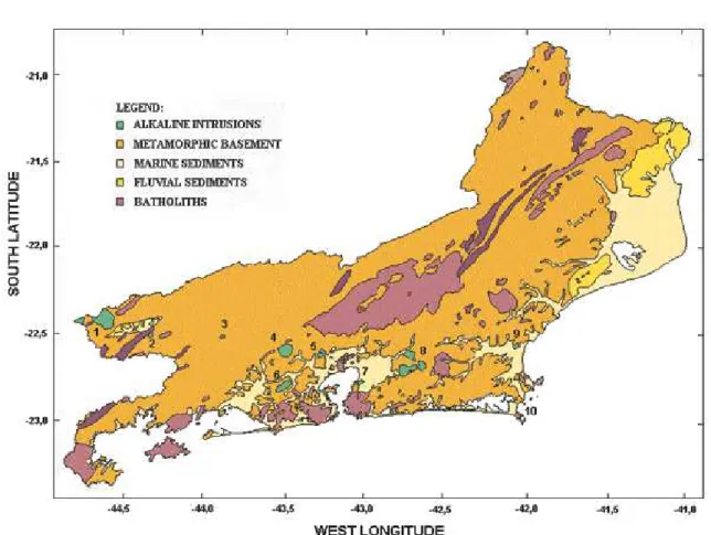
The geological features and tectonic characteristics of the state of Rio de Janeiro have been outlined and discussed in de-tail in the relevant literature (see for example Oliveira et al., 1977; Fonseca, 1998; among others). A simplified version of the geolo-gic map of the study area is reproduced in Figure 1 adapted from CIDE (2002).
Figure 1– Simplified geologic map of the state of Rio de Janeiro, adapted from Centro de Informac¸˜oes e Dados do Rio de Janeiro – CIDE (2002). The numbers indicate the main alkaline intrusions: 1 – Itatiaia; 2 – Resende; 3 – Pira´ı; 4 – Tingu´a; 5 – Cana˜a; 6 – Nova Iguac¸u; 7 – S˜ao Gonc¸alo; 8 – Rio Bonito; 9 – Morro de S˜ao Jo˜ao; 10 – Cabo Frio.
Mendanha and Madureira mountain belts, near the city of Rio de Janeiro.
GEOTHERMAL GRADIENTS
The efforts for determining geothermal gradients began with com-pilation of information on boreholes and wells drilled in the study area. In this stage, extensive use was made of the database for groundwater wells, set up by the Companhia de Pesquisa de Re-cursos Minerais – CPRM. The compilation of CPRM included data on over 4000 wells in the state of Rio de Janeiro. Howe-ver, fewer than 1000 were found to have suitable technical condi-tions (depth range, casing pipes and well head protection) which could potentially guarantee success in eventual geothermal me-asurements. Nevertheless, subsequent field verifications revea-led that a large part of this pre-selected set of wells is equipped with submersible pumps and currently being used for extracting groundwater. As a result successful temperature measurements could be carried out in fewer than 100 wells.
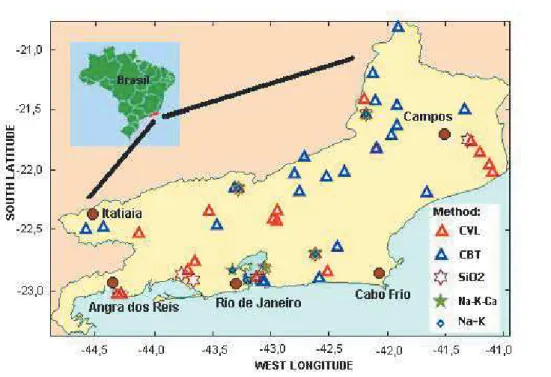
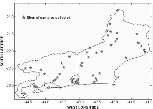
The thermal log data acquired in these wells were used in cal-culating geothermal gradients for 72 localities, distributed in 32 municipalities. The locations of the boreholes and wells where temperature data was acquired are indicated in Figure 2. The geographic distribution of the sites, is rather non-homogeneous, there being large variations in data density in the northern and eastern sectors of the study area.
Field Measurements of Temperatures
Figure 2– Locations of geothermal measurements in the state of Rio de Janeiro. The symbols and letters in the inset indicates the methods used in the determination of geothermal gradients and heat flow. See text for details.
cable allowed corrections for the lead wire resistances of the cable itself. Power supply in the field for the multi-meter and the probe system was provided using a portable battery connected to a DC-AC converter. Color coded markers on the cable were used in de-termination of the depth of the probe during log operations. The thermistor sensor is embedded in a small diameter waterproof me-tallic tube for protection against mechanical vibrations. This tube, made of copper and filled with thermally conductive cement, has a relatively short thermal response time (Roots, 1969). The relation between electrical resistance (R) and absolute temperature (T) of thermistor sensors is generally of the type:
R=R0e
BT1−T10
(1)
whereR0is the resistance at temperatureT0and Ba constant
characteristic of the sensor material. It is common practice to re-cast this equation in the form of a polynomial:
ln(R)=A+ B
T + C
T2 +. . . . (2)
whereA,B,Care coefficients characteristic of the thermistor. The probe system as a whole was calibrated both before and after field operations. During calibration tests the sensor probe is immersed in a temperature controlled water bath. A perfora-ted metallic block inside the water bath was used for housing the
probe. This block acts as a thermal damping device, filtering out high frequency fluctuations generated by the fluid circulation sys-tem of the thermostat. A standard platinum resistance thermo-meter (Presys-ST 501 with ITS 90 specifications) was used for measuring temperatures during calibration tests. The data obtai-ned in calibration tests were employed in the determination of the coefficients (equation 2) of the thermistor response curve.
All measurements were carried out during down-going log operations, avoiding thereby perturbations generated by probe movements inside the borehole. In most cases, measurements were carried out at two meter intervals. This was considered ap-propriate for the present work, in view of the limitations arising from the sensitivity of the probe and of the time spent in field ope-rations. The time interval between positioning of the probe and the final reading was set at 30 to 120 seconds, depending on the ther-mal stability conditions of the temperature field in the borehole.
Determination of Geothermal Gradients
metho-dology and examples of applications are discussed in detail by Hamza & Mu˜noz (1996), Gomes & Hamza (2003), and Hamza et al. (2005b).
The measured values of temperatures need to be corrected for the presence of thermal perturbations. The changes in vege-tation cover and climate conditions of the recent past are known to have significant influence on the temperature field at shallow depths. Incorporation of such corrections are based on models of surface temperature changes and are well-known in the relevant literature (see for example: Hamza, 1991; Shen & Beck, 1991; Hamza, 1998; among others). In the present case, climate correc-tions proposed for the state of Rio de Janeiro by Cerrone & Hamza (2003) were adopted. Temperature variations accompanying ele-vation changes also affect the determination of thermal gradients (Bullard, 1954; 1965). However, calculations carried out by Go-mes (2004) indicate that the topographic corrections are signifi-cant only for six localities, situated in the mountainous regions in the northern part of the study area. The corrections for the effect of thermal disturbances in bore holes, induced by drilling operati-ons, are generally significant only for time periods comparable to the duration of drilling activity (Lachenbruch & Brewer, 1959). In the present case, the elapsed times between conclusion of drilling and temperature log operations were several orders of magnitude larger compared to the periods for drilling shallow wells. Only in one case the corrections for drilling disturbances were found to be significant.
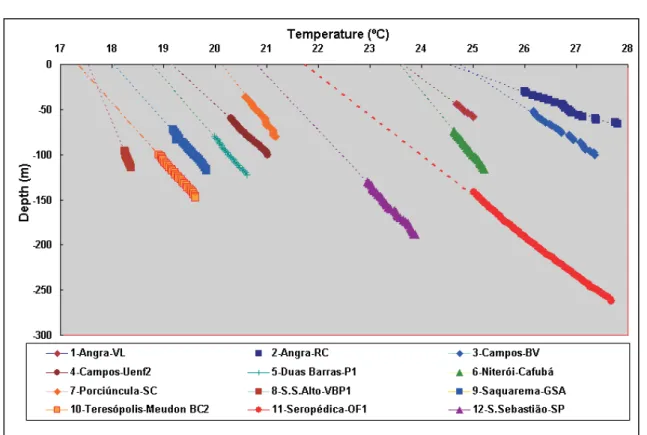
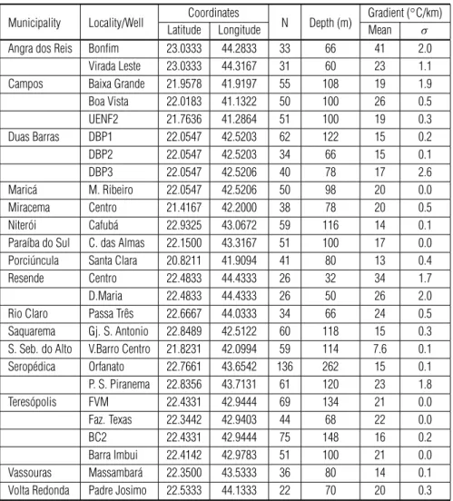
The conventional (CVL) method was employed in cases where the bore holes were found to be in thermal equilibrium and it was possible to identify linear sections in temperature logs indicative of heat transfer by conduction. The temperature gradient was de-termined by least square fit to log data from selected depth inter-vals. The details of the least square techniques are available in standard text books on data analysis (see for example, Bevington, 1969) and its use for determination of temperature gradients in bore holes has been discussed by Ara´ujo (1978). The choice of the depth interval was based on log data and on information from lithologic profiles on the characteristics of the rock types encoun-tered. Example of temperature profiles obtained by the conventi-onal method is illustrated in Figure 3. A summary of geothermal gradients and intercept values obtained by this method is provided in Table 1, along with estimates of the errors (standard deviations in the least square fits) involved. The gradient values obtained are found to fall in the range of 15 to30◦C/km.
In some cases the results of temperature logs reveal that the thermal field of the well is disturbed by water flows occurring in its interior. In such cases the direct use of the conventional method
turns out to be impractical for determination of temperature gra-dients. Nevertheless, an estimate of the gradient may be obtained using temperature data from the bottom-most part of the bore hole where hydraulic perturbations induced by in-hole flows are prac-tically absent. This procedure, designated here as the conventio-nal bottom temperature method – CBT, require knowledge of the mean annual temperature of the surface. In the present case, the temperature data reported for the state of Rio de Janeiro by the Mi-nistry of Agriculture (Minist´erio de Agricultura, 1969) was used. The principle of operation of the CBT method is essentially the same as that of the well-known BHT method, employed in esti-mating temperature gradients in oil wells. The main difference is that in the CBT method the bottom temperatures can be determi-ned with a much greater degree of accuracy than is possible in the BHT method employed in oil well measurements. In addition, high precision repeat measurements may easily be carried out, to verify the nature of drilling disturbances. The results of CBT method are however sensitive to errors in the value of the mean annual surface temperature. Details of the use of this method have been discus-sed by Ribeiro (1987). Examples of temperature profiles obtained by this method are illustrated in Figure 4 and a summary of CBT gradients is provided in part (a) of Table 2. Note that the gradient values by the CBT method are also found to fall in the range of 15 to30◦C/km, in relatively close agreement with those obtained
using the conventional method.
Figure 3– Examples of linear segments of temperature profiles used in the determination of geothermal gradients by the conventional (CVL) method. The bottom inset refers to locations of geothermal measurements.
Table 1– Results of geothermal gradients by the conventional method (CVL).Nis the number of temperature measu-rements andσthe standard deviation.
Municipality Locality/Well Coordinates N Depth (m) Gradient ( ◦C/km)
Latitude Longitude Mean σ
Angra dos Reis Bonfim 23.0333 44.2833 33 66 41 2.0 Virada Leste 23.0333 44.3167 31 60 23 1.1 Campos Baixa Grande 21.9578 41.9197 55 108 19 1.9 Boa Vista 22.0183 41.1322 50 100 26 0.5
UENF2 21.7636 41.2864 51 100 19 0.3
Duas Barras DBP1 22.0547 42.5203 62 122 15 0.2
DBP2 22.0547 42.5203 34 66 15 0.1
DBP3 22.0547 42.5206 40 78 17 2.6
Maric´a M. Ribeiro 22.0547 42.5206 50 98 20 0.0 Miracema Centro 21.4167 42.2000 38 78 20 0.5 Niter´oi Cafub´a 22.9325 43.0672 59 116 14 0.1 Para´ıba do Sul C. das Almas 22.1500 43.3167 51 100 17 0.0 Porci´uncula Santa Clara 20.8211 41.9094 41 80 13 0.4 Resende Centro 22.4833 44.4333 26 32 34 1.7 D.Maria 22.4833 44.4333 26 50 26 2.0 Rio Claro Passa Trˆes 22.6667 44.0333 34 66 24 0.5 Saquarema Gj. S. Antonio 22.8489 42.5122 60 118 15 0.3 S. Seb. do Alto V.Barro Centro 21.8231 42.0994 59 114 7.6 0.1 Serop´edica Orfanato 22.7661 43.6542 136 262 15 0.1 P. S. Piranema 22.8356 43.7131 61 120 23 1.8 Teres´opolis FVM 22.4331 42.9444 69 134 21 0.0 Faz. Texas 22.3442 42.9403 44 68 22 0.0
BC2 22.4331 42.9444 75 148 16 0.2
Barra Imbui 22.4142 42.9783 51 100 21 0.0 Vassouras Massambar´a 22.3500 43.5333 36 80 14 0.1 Volta Redonda Padre Josimo 22.5333 44.1333 22 70 20 0.3
this method is given in part (b) of Table 2. Again, the gradient values are found to fall in the range of 15 to30◦C/km, in
reaso-nably good agreement with those obtained using CVL and CBT methods.
In localities of thermal springs, it is common practice to em-ploy indirect methods of estimating temperature gradients. Ge-nerally techniques of geochemical thermometry are employed in obtaining estimates of the temperature of the deep thermal reser-voir. The basic assumption in this approach is that the dissolution of some of the elements in thermal waters is directly related to the reservoir temperature. Fournier (1981) provides a summary of appropriate relations for the dissolution of Silica, Sodium, Potas-sium and Calcium. These have come to be known popularly as ’geochemical thermometers’, and are used extensively in assess-ment of deep temperatures in hydrothermal systems. The
reser-voir temperature determined in this manner may be combined with the surface temperature in estimating gradients. This approach is usually designated as the geochemical (GCL) method. Hurter et al. (1983) and Hurter (1987) made use of this method in esti-mating temperature gradients for some of the geothermal areas of Brazil.
Table 2– Results of geothermal gradients by (a) the conventional bottom temperature (CBT) and (b) the aquifer temperature (AQT) methods.σis the standard deviation.
(a) – Geothermal gradient values calculated using the CBT method.
Municipality Locality/Well Coordinates Depth(m) Gradient ( ◦C/km)
Latitude Longitude Mean σ
Cambuci Monte Verde 21.4664 41.9197 84 25 2.0 Campos Consel. Josino 21.5006 41.3419 76 21 1.1 S. Sebasti˜ao 21.8539 41.2111 76 37 1.9 Carapebus Centro 22.1869 41.6656 90 30 0.5 Cordeiro Matadouro 22.0169 42.3689 36 34 0.3 Duas Barras DBP4 22.0547 42.5203 78 16 0.2 Itaocara Cel. Teixeira 21.6333 41.9197 76 19 0.1 Jaguaremb´e 21.7133 41.9667 100 17 2.6 Itatiaia Xerox2 22.5000 44.5833 90 17 0.1 Laje de Muria´e Centro 21.2028 42.1250 100 23 0.5 Maric´a Manoel Ribeiro 22.9014 42.5833 76 26 0.1 Manoel Ribeiro 22.9014 42.5833 66 20 0.1 Miguel Pereira Centro 22.4667 43.4667 74 16 0.4 Miracema Para´ıso Tobias 21.4167 42.2000 100 21 1.7 Niter´oi Piratininga 22.9303 43.0500 30 28 2.0 Para´ıba do Sul Ponte Preta 22.1500 43.3167 26 18 0.5 Resende Centro 22.4833 44.4333 50 33 0.3 Rio Bonito Boa Esperanc¸a 22.7931 42.5372 108 33 0.1 S˜ao Gonc¸alo Tribob´o 22.8500 43.0500 18 30 0.1 S.S. do Alto V.Barro-Centro 21.8211 42.0922 106 09 1.8 V.Barro-Centro 21.8242 42.0983 52 07 0.1 Sapucaia Aparecida 22.0322 42.7950 78 14 0.1 Jamapara P3 21.8947 42.7106 74 14 0.2 Jamapara P4 21.8953 42.7086 80 21 0.1
(b) – Geothermal gradient values calculated using the AQT method.
Municipality Locality/Well Coordinates Depth(m) Gradient ( ◦C/km)
Latitude Longitude Mean σ
Teres´opolis ´Agua Quente 22.1786 42.7525 20 64 11.1 Campos S˜ao Sebasti˜ao 21.8539 41.2111 76 35 7.7 Cordeiro Cordeiro 22.0169 42.3689 36 19 5.6
gradient values obtained using the CVL, CBT and AQT methods.
Quality Considerations of the Methods used for Temperature Gradients
The quality considerations of the available data set are, in part, related to the characteristics of the methods used for determining gradients, which in turn depend on the nature and availability of primary temperature data. In an attempt to minimize problems ari-sing from the use of data sets of mixed quality Hamza & Mu˜noz
compa-Table 3– Estimates of geothermal gradients based on the geochemical (GCL) method for the Silica (a), Na-K (b) and Na-K-Ca (c) geothermometers.σrepresents the standard deviation.
(a) – Estimates using the Silica thermometer (SiO2)
Municipality Locality/Spring Coordinates Gradient ( ◦C/km)
Latitude Longitude Mean σ
Campos Pedra Alecrim 21.7500 41.3167 34 0.4 Itagua´ı Poc¸o 2 22.8667 43.7667 49 0.3 Niter´oi Ing´a 22.8961 43.1203 60 0.3 Para´ıba do Sul Salutaris 22.1500 43.2833 46 0.3 Rio Bonito Catimbau 22.7000 42.6167 69 0.2 Rio de Janeiro Santa Cruz 22.9167 43.2167 29 0.2 St. A. de P´adua Iodetada 21.5333 42.1833 45 0.2 S. Gonc¸alo Ag. S. Gonc¸alo 22.8167 43.0500 51 0.3
(b) – Estimates using the Sodium – Potassium thermometer (Na-K).
Municipality Locality/Spring Coordinates Gradient ( ◦C/km)
Latitude Longitude Mean σ
Para´ıba do Sul Salutaris 22.1500 43.2833 26 8.4 Rio Bonito Catimbau 22.7000 42.6167 69 7.2 Rio de Janeiro ´Agua Meyer 22.6667 43.5833 70 7.4 Nazareth 22.9167 43.2167 57 7.3 Silva Manuel 22.9167 43.2167 24 5.3 St. A. de P´adua Iodetada 21.5333 42.1833 31 5.8
(c) – Estimates using the Sodium-Potassium-Calcium thermometer (Na-K-Ca).
Municipality Locality/Spring Coordinates Gradient ( ◦C/km)
Latitude Longitude Mean σ
Para´ıba do Sul Salutaris 22.1500 43.2833 41 1.3 Rio Bonito Catimbau 22.7000 42.6167 69 1.8 Rio de Janeiro ´Agua Meyer 22.6667 43.5833 64 1.7 Silva Manuel 22.9167 43.2167 29 1.4 St. A. de P´adua Iodetada 21.5333 42.1833 45 1.4 S. Gonc¸alo Ag. S. Gonc¸alo 22.8167 43.0500 51 1.5
rative analyses of repeat temperature logs, carried out before and after blockage of hydraulically active fracture zones in bore ho-les. However, cementing operations capable of blocking in-hole flows are expensive and not practical in many cases. Hamza et al. (2005b) suggested a relatively simple procedure that provi-des indirect checks on the reliability of this method. In this case, a comparison is made of the gradient values by the CBT method with those obtained by the conventional (CVL) method for undis-turbed bore holes, situated in the same general region as that of the boreholes with hydraulic disturbances. According to Hamza et al. (2005b) the use of CBT method leads to errors of less than 4% in the determination of gradients in the interval of 5 to50◦C/km.
gradi-ents are less than 2%. For the purposes of the present work, the results of these comparisons were considered as satisfactory and the AQT method is classified as occupying the third position in the priority list.
The results of geochemical methods, when compared with those of the other methods, appear to provide overestimates of the temperature gradients. It is, however, likely that the locali-ties of thermal springs, being discharge areas of thermal fluids, are inherently characterized by relatively higher thermal gradients. Measurements in deep holes using conventional methods are ne-cessary to understand the true nature of thermal field in localities of thermal springs. Another major source of uncertainty in GCL methods arises from the methods used in estimating the depth of circulation of thermal fluids. These estimates are usually based on inferences as to the structural setting of the crustal blocks and of the aquifers. Because of such inherent uncertainties the results of the geochemical (GCL) method has been assigned the least pri-ority. The estimates by geochemical method are taken into con-sideration only for localities where other more reliable methods have failed to provide satisfactory results.
Analysis of data presented in Tables 1 to 3 reveal that there is considerable variability in local geothermal gradients. Such vari-ability may arise either as a result of advective heat transport by subsurface fluid flows or as a consequence of local thermal re-fraction effects. Preliminary calculations indicate that the effects of thermal refraction are unlikely to be significant, except in very specific cases of structural complexity. On the other hand, there are indications of the existence of water flow at shallow depths in many localities. Detailed information on groundwater flow pattern is however necessary to evaluate the role of advective heat transfer on local and regional scales.
Local and Regional Variations in Geothermal Gradients
As noted earlier, the temperature gradients obtained by the CVL method are in reasonable agreement with those found for the CBT and AQT methods. On the other hand, the estimates of gradients obtained by the GCL method are found to fall in a slightly higher range. The possible existence of systematic difference between the GCL and the other methods is a matter of concern and ma-kes the interpretation of regional distribution a difficult task. To circumvent this problem, two different data sets were considered: first one based exclusively on the relatively more reliable CVL, CBT and AQT data and a second one of mixed quality that include also the GCL data.
Maps of the regional distribution of temperature gradients were produced using both commercially available (SURFER) and public domain (GMT) automatic contouring programs. The soft-ware routines available in these graphic utility packages were em-ployed in testing a variety of schemes for grid spacing, data in-terpolation and contouring procedures. The regional geothermal gradient map based on the CVL, CBT and AQT data sets is presen-ted in Figure 5. It reveals that the temperature gradients are low to normal (in the range of 10 to30◦C/km) mainly in the eastern
parts of the state of Rio de Janeiro. On the other hand, gradient values higher than30◦C/km are found in the western parts. The
distinct difference in the distribution of thermal gradients between the eastern and western parts of the study area may be considered as an important feature of the regional geothermal field.
In some localities such as Niter´oi, S˜ao Gonc¸alo, Jamapar´a (Sapucaia), ´Agua Quente and Silva Jardim the gradients are found to be higher than50◦C/km. These values appear as isolated
ano-malies and are based on measurements carried out in very shal-low wells. In the absence of supplementary data from deep wells we consider it as unwise to attach overdue significance to such observations.
The regional gradient map for the mixed data set which inclu-des also the estimated values by the GCL method is presented in Figure 6. In this case temperature gradients with values higher than30◦C/km are found to occur over a much larger area. It is
important to note that many of the high gradient areas are coin-cident with the localities of thermal and mineral springs. There are, however, indications of an approximate east – west trend in the gradient anomaly, which is nearly coincident with the belt of alkaline intrusions of Tertiary age.
THERMAL CONDUCTIVITY MEASUREMENTS
Figure 5– Regional distribution of geothermal gradients based on selected data sets (CVL, CBT and AQT methods). See text for details.
Figure 6– Regional distribution of geothermal gradients based on the complete data set that include also estimates by the GCL method.
In many cases, drilling operations were completed during the de-cades of 1970 and 1980 and this also contributed to difficulties in obtaining representative samples. In an attempt circumvent such problems fresh unaltered samples taken from outcrops of the main geologic formations were used as supplementary material for ther-mal conductivity measurements. The sample collection was car-ried out by the Geology Department of the State University of Rio de Janeiro (UERJ). The localities from which samples were
ob-tained for conductivity measurements are indicated in the map of Figure 7. The sites of outcrops are not always close to the locali-ties of gradient data, a consequence of problems encountered in acquisition of representative samples of the geologic formations.
Experimental Procedures
Figure 7– Map indicating sites of samples used for thermal conductivity measurements.
Observat´orio Nacional – ON. Two different experimental techni-ques were employed, designated here as the line source and the plane source methods. These are in fact transient methods where the thermal conductivity is evaluated by monitoring the growth and decay of thermal perturbations induced in the sample. The principle of the line source method is well known (see for exam-ple, Carslaw & Jaeger, 1959) and its application for measurements with geologic materials in Brazil has been discussed in detail by Hamza et al. (1980) and Marangoni (1986). The sensor probes of the line source method allow two different heat dissipation geo-metries, depending on the physical characteristics of the samples. For measurements in unconsolidated materials the probe is inser-ted into the sample. In this case the dissipation of heat then occurs in what is termed as the full-space or4πgeometry. In the case of
solid cores and consolidated materials, the probe of line source is glued onto the smooth surface of a reference plate and brought into contact with a smooth surface of the sample. If the reference plate is a thermal insulator the heat dissipation is considered as occurring under what is termed as half-space or2π geometry.
The experimental setup used in the line source methods is similar to the ones employed in earlier studies by Hamza et al. (1980) and Marangoni (1986).
The use of experimental devices employing plane sources of heat, operating under transient thermal regime, is less frequent. Carslaw & Jaeger (1959) discuss the theory of the plane source method in detail. The temperature(T)variation at a distance(x)
with time(t)of a sample of thermal conductivity(λ)in contact with a continuous plane source of heat is given by:
T =Q
tρc π λ
1/2
e−(x−x ′)2
4κt − Q|x−x ′|
2κρc er f c
|x−x′|
2√κt (3)
whereQis the strength of heat source,(ρC)the heat capacity andκthe thermal diffusivity. Mongelli (1968) reported results of experimental studies on rock samples using this method. In the present work, a commercially available instrument (ISOMET 104, Applied Precision Ltd., Slovak Republic) was used. It is equipped with a microprocessor device, which carries out integration of the time – temperature curves and provides a display of the calculated value of thermal conductivity. Integration of the thermal response is carried out during both the heating and cooling cycles.
Both primary and secondary standards were used in calibra-ting the measurement devices. The primary standards used are fused silica and crystalline quartz discs. These are usually consi-dered as reference materials with internationally accepted values of thermal conductivity. The secondary standards include selected engineering materials and discs of rock samples whose thermal conductivity values are known from inter-laboratory comparison studies.
Variation with Rock Types
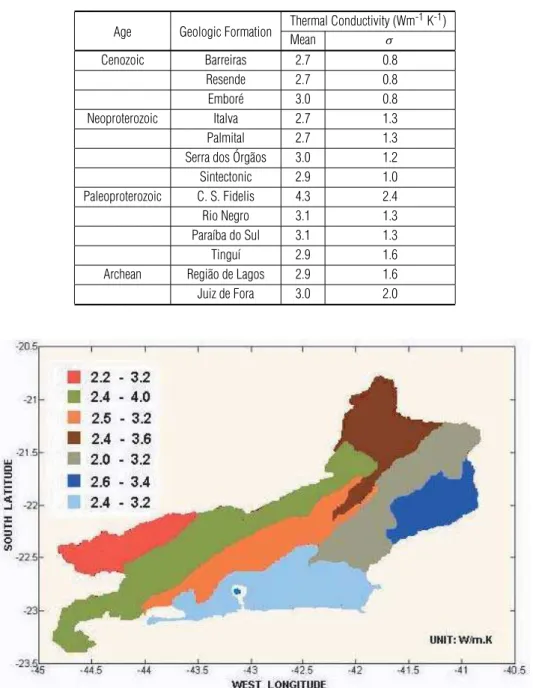
carried out in which the mean values of the main geologic forma-tions were determined. The procedure adopted in this case relies not only on the use of experimental data but also on information available in detailed geologic maps of the localities. Thus weigh-ted mean values of thermal conductivity of the main geologic for-mations occurring within the study area were calculated. The set of such values, reproduced in Table 4, reveal that the geologic for-mations of Neoproterozoic age are characterized by mean thermal conductivity values in the range of 2.7 to 3.0 Wm-1K-1. On the
other hand, the basement rocks of Paleoproterozoic and Archean ages appear to be characterized by slightly higher values, in the range of 2.9 to 4.3 Wm-1K-1. The sedimentary rock formations
of Mesozoic and Tertiary periods are found to have relatively low thermal conductivity, in the range of 2.2 to 3.2 W m-1K-1.
The data in Table 4 may also be used for examining the large-scale inter-formational variations in thermal conductivity. For example, the map of Figure 8 illustrates the regional distribu-tion of mean thermal conductivity values of the main geologic formations. It reveals a pattern similar to that depicted in geo-logic maps of the study area, a consequence of the implicit as-sumption that thermal conductivity is constant within any speci-fic geologic formation. The weakness of this approach is that it amounts to a strong averaging procedure and ignores eventual intra-formational variations in thermal conductivity.
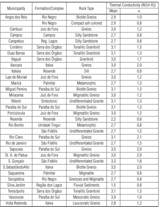
A better approach in evaluation of regional variations in ther-mal conductivity is to relate the available experimental data to the lithologic sequences encountered in the wells and petrologic des-criptions of outcrops. This allows representative values of thermal conductivity to be assigned to the main rock types. Such repre-sentative values and their associated uncertainties are listed in Table 5. As can easily be verified, the metamorphic rocks of the basement complex in the northern parts are characterized by ther-mal conductivity values in the range of 2.8 to 4.3 Wm-1K-1. This
range is slightly higher than that encountered for rocks of the co-astal complex in the south. As expected, the acidic rocks (granites, granitoids and migmatite sequences) have thermal conductivities higher than those of the basic rocks (gabbro and basalt). On the other hand relatively low values, in the range of 1 to 2 Wm-1K-1,
were encountered for unconsolidated sediments and soil samples.
The data in Table 5 also allow evaluation of large-scale regi-onal variations in thermal conductivity. Thus the map of Figure 9 illustrates the regional distribution of mean thermal conductivity values of the main lithologic units in the study area. Note that the thermal conductivity is relatively high in the region adjacent to the S˜ao Francisco craton, in the northern parts of the study area.
Site Specific Mean Values
The data presented in Tables 4 and 5 also allow calculation of weighted mean thermal conductivity values for the sites for which geothermal gradients were calculated. Such values of thermal conductivity are important in the calculation of site specific heat flow values. However, the procedure for calculation of the site specific mean thermal conductivity depends on the method used for the determination of geothermal gradients. Thus, for those si-tes where the conventional (CVL) method was used, a mean value of thermal conductivity was calculated for the relevant depth sec-tion. On the other hand, for sites where the CBT method was used for determining temperature gradients, the mean value of thermal conductivity calculated refers to the entire lithologic sequence en-countered, from the surface down to the bottom of the well. The site specific values of thermal conductivity calculated in this man-ner are presented in Table 6.
Note that the overall mean thermal conductivity for the 32 sites, where thermal gradients were determined using the CVL method, is 3.0 Wm-1K-1. On the other hand for the 22
si-tes, for which thermal gradients were calculated using the CBT method, the overall mean value of thermal conductivity is only 2.6 Wm-1K-1. The relatively low value for the CBT sites is due to the
inclusion of low thermal conductivities of partially consolidated materials in near surface layers.
DETERMINATION OF HEAT FLOW VALUES
All heat flow values reported in the present work are based on the assumption that the thermal regime of the study area is in steady state. In tectonically stable areas of the continental crust transient changes in the thermal regime take place on time scales that are too large for human experiments. Thus the assumption of steady state is quite reasonable.
Methods used in determination of Heat Flow
In the present work four different methods were employed in deter-mining heat flow, depending on the nature of temperature gradient and thermal conductivity data. The terminology adopted here fol-lows that used for the case of temperature gradients. Thus the designations conventional (CVL), conventional bottom tempera-ture (CBT), aquifer temperatempera-ture (AQT) and geochemical (GCL) are also retained for the methods of determining heat flow.
Table 4– Mean thermal Conductivity values of the main geological formations in the study area.σis the standard deviation.
Age Geologic Formation Thermal Conductivity (Wm -1K-1)
Mean σ
Cenozoic Barreiras 2.7 0.8
Resende 2.7 0.8
Embor´e 3.0 0.8
Neoproterozoic Italva 2.7 1.3
Palmital 2.7 1.3
Serra dos ´Org˜aos 3.0 1.2 Sintectonic 2.9 1.0 Paleoproterozoic C. S. Fidelis 4.3 2.4
Rio Negro 3.1 1.3
Para´ıba do Sul 3.1 1.3
Tingu´ı 2.9 1.6
Archean Regi˜ao de Lagos 2.9 1.6 Juiz de Fora 3.0 2.0
Figure 8– Thermal conductivity structure of the main geologic formations in the state of Rio de Janeiro. The inset refers to thermal conductivity values in units of Wm-1K-1.
harmonic mean of thermal conductivity(λm):
q=Γ λm±σq (4)
The error estimate in heat flow,σq, is given by the relation for
error propagation:
σq=
Γ2σ2 λ +λ
2σ2
Γ (5)
σλ is the standard deviation in the determination ofλandσΓ
is the standard deviation in the determination of temperature gra-dient. As mentioned in the previous section (see also Table 6) the value ofλmwas calculated making use of experimental data
Table 5– Mean thermal conductivity values of the main rock types.σis the standard deviation.
Municipality Formation/Complex Rock Type Thermal Conductivity (W/(m K))Mean
σ
Angra dos Reis Rio Negro Biotite Gneiss 2,9 1,0 Rio Negro Compact ash colored 2,9 0,8
Cambuci Juiz de Fora Gneiss 3,0 1,2
Campos Campos Silty Sandstone 2,7 0,8
Carapebus Reg. Lagos Silty Sandstone 2,7 0,8 Cordeiro Serra dos ´Org˜aos Tonalitic Granitoid 3,1 1,3 Duas Barras Serra dos ´Org˜aos Tonalitic Granitoid 3,1 1,3 Itagua´ı Serra dos ´Org˜aos Granitoid 3,0 1,7
Itaocara Italva Gneiss 3,0 2,0
Itatiaia Resende Silt 2,7 0,8
Laje de Muria´e Juiz de Fora Gneiss 3,0 1,2
Maric´a Palmital Metamorphic 2,7 1,3
Miguel Pereira Para´ıba do Sul Biotite Gneiss 3,1 1,3 Miracema Juiz de Fora Migmatitic Gneiss 3,0 1,2 Niter´oi Sintectonic Undifferentiated Granite 3,1 1,3 Para´ıba do Sul Para´ıba do Sul Biotite Gneiss 3,1 1,3 Porci´uncula Juiz de Fora Migmatitic Gneiss 3,0 1,2
Resende Resende Silty Sandstone 2,2 0,8
Rio Bonito Unidade Tingui Metamorphic 2,7 0,8 S˜ao Fid´elis Undifferentiated Granite 2,7 1,5 Rio Claro Para´ıba do Sul Gneiss 3,1 2,1 Rio de Janeiro S˜ao Fid´elis Undifferentiated Granite 2,7 1,5
Sapucaia Para´ıba do Sul Gneiss 3,5 2,0
St. A. de P´adua Juiz de Fora Migmatitic Gneiss 3,0 2,0 S. Gonc¸alo S˜ao Fid´elis Undifferentiated Granite 3,3 1,8 S.Sebasti˜aodoAlto Italva Biotite Gneiss 3,5 2,0
Saquarema Palmital Migmatite 2,7 0,8
Serop´edica Rio Negro Gneisses and Migmatite 2,7 0,8 Silva Jardim Regi˜ao dos Lagos Fluvial Sediments 1,5 0,8 Teres´opolis Serra dos ´Org˜aos Tonalitic Granitoid 3,1 1,3 Vassouras Para´ıba do Sul Mesocratic Gneiss 3,9 1,0 Volta Redonda Italva Leucocratic Gneiss 2,8 1,2
method is provided in Table 7, along with estimates of the errors involved. Note that the values are found to fall in the range of 30 to 60 mW/m2.
In the conventional bottom temperature (CBT) method the heat flow(q)is calculated as product of the CBT gradient(ΓCBT)
and weighted mean thermal conductivity:
q =
(T
C BT −T0) (ZC BT −Z0)
(Z
C BT −Z0) N i=1Rihi
(6)
whereTC BT is the temperature at depth ZC BT, Ris the
ther-mal resistivity of the layer with thicknesshandnthe number of layers. Note that the first term on the right hand side of equa-tion (6) represent the CBT gradient while the second term in curly brackets represent the weighted mean thermal conductivity of all the layers within the depth interval(ZC BT −Z0). Obviously,
Figure 9– Regional distribution of thermal conductivity values of the main rock types in the state of Rio de Janeiro. The inset refers to contour values are in units of W/mK.
with those obtained using the conventional method.
In the aquifer temperature (AQT) method the heat flow(q)is calculated using a relation similar to that of equation (6):
q =
(T
A QT −T0) (ZA QT −Z0)
(Z
A QT −Z0) N i=1Rihi
(7)
whereTA QT is the temperature at depthZA QT,Ris the thermal
resistivity of the layer with thicknesshandnthe number of layers. Note that the first term on the right hand side of equation (7) re-present the AQT gradient while the second term in curly brackets represent the weighted mean thermal conductivity of all the layers within the depth interval(ZA QT−Z0). A summary of heat flow
obtained by the AQT method is given in part (b) of Table 8. The values are found to fall in the range of 30 to 70 mW/m2, in
relati-vely close agreement with those obtained using the conventional method.
In areas of thermal springs heat flow is estimated using the empirical relation:
q =(TR−T0)
λ
ZR
(8)
whereTR is the reservoir temperature at depth ZR, estimated
using one of the geochemical thermometers and T0the mean
annual surface temperature. Note that the inverse of the term
(λ/ZR)represents the cumulative thermal resistance of the layer
overlying the hydrothermal system. Swanberg & Morgan (1979)
proposed a value of680◦Cm2/W for the thermal resistance term,
for areas where silica thermometer is employed for estimating re-servoir temperatures. Note that this approach implicitly assumes a depth of circulation of approximately 2 km for the thermal waters. A summary of heat flow obtained by the geochemical method (GCL) is provided in Table 9. Note that the values obtained are in the range of 30 to 150 mW/m2, significantly higher than those
obtained by CVL, CBT and AQT methods. It is possible that this is a consequence of the tendency to overestimate temperature gradi-ents in the geochemical method. On the other hand, the possibility that the localities of thermal springs are characterized by higher heat flow at deeper depths cannot entirely be ruled out. Measu-rements in deep holes using conventional methods are necessary to verify this possibility.
Regional Variations
The heat flow data presented in Tables 7 to 9 were used in exa-mining the regional distribution of heat flow. As in the case of thermal gradients, two different data sets were considered: one based exclusively on the relatively more reliable CVL, CBT and AQT data and the other one of mixed quality that include also the less reliable GCL estimates.
Table 6– Mean thermal Conductivity (λ)values of the sites where CVL (selected interval) and CBT (whole interval) methods were used in determination of gradients. The values are in units of W/(m.K).σis the standard deviation.
Locality λfor selected interval Locality λfor whole interval
Mean σ Mean σ
Bonfim 2,9 0,58 Monte Verde 2,8 0,42 Virada Leste 2,9 0,64 Consel. Josino 2,3 0,35 Baixa Grande 2,7 0,54 Carapebus 2,2 0,33 Boa Vista 2,7 0,59 Matadouro 2,5 0,38 S˜ao Sebasti˜ao 2,2 0,44 Duas Barras-DBP4 3,0 0,45 Uenf 2 3,0 0,60 Cel. Teixeira 2,6 0,39 Duas Barras-DBP1 3,1 0,61 Jaguaremb´e 2,6 0,39 Duas Barras-DBP2 3,1 0,67 Pr´oximo Dutra 2,2 0,33 Duas Barras-DBP3 3,1 0,64 Laje do Muria´e 3,0 0,45 Manoel Ribeiro 2,7 0,53 Maric´a-M.RibeiroP1 2,5 0,38 Miracema 3,0 0,60 Maric´a-M.RibeiroP3 2,6 0,39 Cruz das Almas 3,1 0,62 Miguel Pereira 2,7 0,41 Santa Clara 3,0 0,60 Para´ıso Tobias 3,0 0,45
Resende-P2 2,7 0,54 Cafub´a 3,0 0,48
Resende-D. Maria 2,7 0,59 Piratininga 2,7 0,41 Passa Trˆes 3,1 0,62 Ponte Preta 1,7 0,26 Aparecida 3,5 0,70 Resende–P1 2,7 0,41 Jamapara-P3 3,5 0,77 Boa Esperanc¸a 2,8 0,42 Jamapara-P4 3,5 0,74 Aparecida 2,9 0,44
Tribob´o 3,1 0,62 Jamapara 2,9 0,44
S.S. do Alto–P1 3,5 0,70 Faz. Brasil 1,4 0,21 S.S. do Alto–P2 3,5 0,77 ´Agua Quente 2,4 0,36
S.S. do Alto–P3 3,5 0,74 – – –
Gj. S. Antonio 2,7 0,54 – – –
Orfanato 2,7 0,57 – – –
P.S.Piranema 2,7 0,59 – – –
Meudon-BC2 3,1 0,67 – – –
Faz. Texas 3,1 0,61 – – –
Meudom 3,1 0,64 – – –
Barra do Imbui 3,1 0,61 – – –
Massambar´a 3,9 0,78 – – –
Padre Josimo 2,8 0,56 – – –
interior of the state of Rio de Janeiro, especially in the northern re-gions just to the south of S˜ao Francisco Craton. Heat flow values lower than 40 mW/m2 was encountered only in three localities
in the municipality of S˜ao Sebasti˜ao do Alto. The overall pattern of heat flow distribution is similar that observed for the tempe-rature gradients. This is an indication that thermal conductivity variations have only a secondary and subdued effect on regional distribution of heat flow.
Heat flow values higher than 80 mW/m2were found in the
western parts of the study area, in the region adjacent to the alka-line intrusion of Itatiaia and also in the Resende sedimentary ba-sin. The western and southern boundaries of this heat flow ano-maly are not well defined for lack of appropriate data. However, there are some indications that areas with heat flow higher than 80 mW/m2extend along the belt of alkaline intrusions between
Table 7– Heat flow values calculated using the conventional (CVL) method.σis the standard deviation.
Municipality Locality Heat Flow (mW/m 2)
Mean σ
Angra dos Reis Bonfim 119 15.4 Virada Leste 67 8.6 Campos Baixa Grande 51 8.0 Boa Vista 70 8.5
UENF2 57 6.9
Duas Barras DBP1 46 5.5
DBP2 46 5.5
DBP3 52 10.1
Maric´a M. Ribeiro 53 6.4 Miracema Centro 60 7.4 Niter´oi Cafub´a 43 5.2 Para´ıba do Sul C. das Almas 53 6.3 Porci´uncula Santa Clara 39 4.8 Resende Centro P2 92 11.9
D.Maria 70 10.0 S.Seb.do Alto V.Barro-P1 26 3.6
Saquarema Gj. S. Antonio 41 4.9 Serop´edica Orfanato 62 7.5 P.S.Piranema 59 7.1 Teres´opolis FVM 64 9.5 Faz. Texas 67 8.1
BC2 49 5.9
Barra Imbui 64 7.7 Vassouras Massambar´a 55 6.6 Volta Redonda Padre Josino 56 6.7
The regional heat flow map based on the complete data set, that includes also estimates by GCL methods, is presented in Fi-gure 11. In this case the zone of high heat flow (>80mW/m2)
extends over a much larger area in the western parts, a region affected by alkaline magmatism during the Tertiary period. It ap-pears that the heat flow regime of the eastern part of the study area is distinctly different from that of the western part. One of the most likely process responsible for this difference is the residual heat from the Tertiary alkaline magmatic activity. According to Smith and Shaw (1975) residual heat from intrusive magmatism at intra-crustal layers may constitute a significant component of near sur-face conductive heat flux for periods of up to 100 m.y. Recently Hamza et al. (2005a) presented calculations of residual heat from Trindade plume, based on the model of hot spot in a moving me-dium proposed by Birch (1975). The calculations indicate that for relative velocities of less than one centimeter per year, the
trai-ling part of the hot spot trajectory may retain significant amount of residual heat in lower to mid crustal layers.
DISCUSSION AND CONCLUSIONS
The results obtained in the present work indicate that the geother-mal gradients in most parts of the state of Rio de Janeiro fall in the interval of 15 to30◦C/km. The mean value is20.5±7.2◦C/km,
typical of the gradients commonly encountered in tectonically inactive areas of Precambrian age. Regional distribution as reve-aled in geothermal maps indicate that the temperature gradients are relatively high (>30◦C/km) in the western parts compared
to the eastern parts of the study area.
Table 8– Heat flow values by the conventional bottom temperature (CBT) and aquifer temperature (AQT) methods.σis the standard deviation.
(a) – Heat flow values calculated using the CBT method.
Municipality Locality Heat Flow (mW/m 2)
Mean σ
Cambuci Monte Verde 70 9.0 Campos Consel. Josino 49 7.8 S˜ao Sebasti˜ao 55 8.7 Carapebus Centro 67 10.1
Cordeiro Matadouro 83 12.4 Duas Barras Centro DBP4 48 7.2
Itaocara Cel. Teixeira 50 7.5 Jaguaremb´e 45 9.6 Itatiaia Pr´oximo Dutra 36 5.5 Laje de Muria´e Centro 70 10.6
Maric´a Manoel Rib - P1 64 9.6 Manoel Ribeiro 41 6.1 Miguel Pereira Centro 44 6.7 Miracema Para´ıso Tobias 61 10.5
Niter´oi Piratininga 75 12.6 Para´ıba do Sul Ponte Preta 29 4.4
Resende Centro P1 65 9.8 Rio Bonito Boa Esperanc¸a 92 13.8 S˜ao Gonc¸alo Tribob´o 78 11.7 S˜ao Seb. do Alto V.Barro-VBP2 24 5.9
V.BarroVBP3 21 3.2 Sapucaia Aparecida 41 6.2 Jamapara P3 41 6.2 Jamapara P4 61 9.1
(b) – Heat flow values calculated using the AQT method.
Municipality Locality Heat Flow (mW/m 2)
Mean σ
Teres´opolis ´Agua Quente 111 57.9 Campos S˜ao Sebasti˜ao 95 29.9 Cordeiro Cordeiro 61 26.0
The underlying mechanism for the occurrence of such a trend is not entirely clear, in view of the limitations of the data set. On the other hand, the crustal segments of the northern parts are relati-vely more deeply eroded than the southern counterparts. The deep seated rocks are in general of relatively higher metamorphic grade and density, less porous and more compact. These are also condi-tions that favor relatively higher thermal conductivity. Hence, the observed trend of decreasing values in the north-south direction is likely to be indicative of a direct correlation between thermal
conductivity and metamorphic grade.
The mean value of heat flow by the conventional method is
64±28mW/m2. Most of the individual values are found to fall
in the interval of 40 to 80 mW/m2, a range that may be considered
as typical of continental crust. Nevertheless, the regional distri-bution reveals that heat flow is relatively high (>80mW/m2) in
Table 9– Heat flow by the geochemical (GCL) method. The column under the letters GT indicates the type of geochemical thermometer.σis the standard deviation.
Municipality Spring Geothermometer Heat Flow (mW/m 2)
q σ
Campos Pedra Alecrim SiO2 54 6.6
Itagua´ı Poc¸o 2 SiO2 88 10.6
Niter´oi Ing´a SiO2 108 13.0
Para´ıba do Sul Salutaris SiO2 84 33.8 Salutaris Na-K-Ca 84 33.8
Salutaris Na/K 84 10.1
Rio Bonito Catimbau SiO2 108 12.9 Catimbau Na-K-Ca 108 13.1
Catimbau Na/K 108 23.3
Rio de Janeiro Agua Meyer Na-K-Ca 100 12.0 Agua Meyer Na/K 100 12.0
Nazareth Na/K 120 26.9
Santa Cruz SiO2 78 9.4
Silva Manuel Na/K 73 16.7 Silva Manuel Na-K-Ca 73 9.5 S. A. de P´adua Iodetada SiO2 78 9.4 Iodetada Na-K-Ca 78 10.2
Iodetada Na/K 78 19.8
Ag. S. Gonc¸alo SiO2 99 11.9 Ag. S. Gonc¸alo Na-K-Ca 99 12.8
Figure 11– Regional heat flow map based on the complete data set that includes also estimates by the GCL method.
At present heat flow data are available for 72 localities which mean that the overall data density for the state of Rio de Janeiro is one per 600 square kilometers area. This may appear as too low but it is useful to note that it is more than an order of magni-tude higher than the global heat flow data density. According to current statistics Rio de Janeiro stands out as the state with the highest data density for geothermal measurements in Brazil. Ne-vertheless, the limit of spatial resolution in heat flow maps is no better than several tens of kilometers. This may be considered sa-tisfactory for regional heat flow investigations, but is still too low if comparative studies are to be undertaken against other ground based gravity and magnetic data.
Finally, it is convenient to keep in mind the main limitations of the database. The current geographic distribution of geother-mal database is somewhat non-homogeneous, there being several areas in the eastern and western parts of the State for which re-levant data are not available. Most of the data has been acquired in bore holes and wells with depths less than a few hundred me-ters. Lack of availability of deep drill holes has not allowed direct measurements at depths reaching into the mid sections of the up-per crust. Thus the conclusions of this work should be viewed in proper perspective, subject to confirmation by measurements in deeper drill holes.
ACKNOWLEDGEMENTS
The geothermal project of the State of Rio de Janeiro, which served as the background for heat flow measurements, received support
from Fundac¸˜ao Amparo `a Pesquisa do Estado do Rio de Janeiro – FAPERJ (Process noE-26/151. 920/2000). A large part of the
samples used for thermal conductivity measurements were obtai-ned from the Geology Department of the State University of Rio de Janeiro – UERJ. The first author of this paper has been a recipient of a scholarship granted by Coordenadoria de Aperfeic¸oamento de Pesquisa e Ensino Superior – CAPES, during the period 2001 – 2003.
REFERENCES
ALMEIDA FFM. 1967. Origem e evoluc¸˜ao da Plataforma Brasileira, Bo-letim DGM/DNPM, Rio de Janeiro, Brasil.
ALMEIDA FFM. 1977. O Cr´aton do S˜ao Francisco, Revista Brasileira de Geociˆencias, S˜ao Paulo, 23(7): 349–364.
ALMEIDA FFM. 1991. O alinhamento magm´atico de Cabo Frio, II Simp´osio de Geologia do Sudeste, S˜ao Paulo, Atas, p. 423–428.
ALMEIDA FFM, HASUI Y & CARNEIRO CDR. 1975. O lineamento de Al´em Para´ıba, Anais da Academia Bras. Ciˆenc. Res. Comum. 47(3/4): 575.
ARA ´UJO RLC. 1978. Pesquisas de fluxo t´ermico na chamin´e alcalina de Poc¸os de Caldas, Tese de Mestrado, Universidade de S˜ao Paulo, S˜ao Paulo, Brasil.
BEVINGTON PR. 1969. Data reduction and error analysis for the physical sciences, McGraw-Hill, New York.
BOLDITZAR T. 1958. The distribution of temperature in flowing wells. Am. J. Sci., 256: 294–298.
BULLARD EC. 1954. The flow of heat through the floor of the Atlantic Ocean. Proc. R. Soc. London A, 222: 408–429.
BULLARD EC. 1965. Historical introduction to terrestrial heat flow, in: LEE WHK (Ed.), Terrestrial Heat Flow, Geophys. Mon. No. 8, 1–6, Ame-rican Geophysics Union, Washington.
CARSLAW HS & JAEGER JC. 1959. Conduction of heat in solids, Cla-rendon Press, Oxford.
CENTRO DE INFORMAC¸ ˜OES E DADOS DO RIO DE JANEIRO – FUNDAC¸˜AO CIDE. 2002. Mapa Geol´ogico do Estado do Rio de Janeiro. Dispon´ıvel em: < http://www.cide.rj.gov.br/download/territorio/territo-rios.asp>Acesso em: jun. 2002.
CERRONE BN & HAMZA VM. 2003. Variac¸˜oes paleoclim´aticas no Es-tado do Rio de Janeiro com base no m´etodo geot´ermico,8◦International Congress of the Brazilian Geophysical Society, Rio de Janeiro.
FONSECA MJG. 1998. Mapa Geol´ogico do Estado do Rio de Janeiro, Es-cala 1:400.000, Publicac¸˜ao Departamento Nacional da Produc¸˜ao Mineral (DNPM), Bras´ılia (DF).
FOURNIER RO. 1981. Application of water geochemistry to geothermal exploration and reservoir engineering, In Geothermal Systems: Princi-ples and Case Histories, RYBACH L & MUFFLER LJP. (Eds.), Wiley, New York, 109–143.
FREITAS RO. 1944. Jazimento de rochas alcalinas no Brasil Meridional, Min. Met., 8(43): 45–48.
GIGGENBACH WF. 1988. Geothermal solute equilibria. Derivation of Na-K-Mg-Ca geoindicators. Geochim. Cosmochim. Acta, 52: 2749–2765.
GOMES AJL. 2004. Avaliac¸˜ao de Recursos Geotermais do Estado do Rio de Janeiro, Tese de Mestrado, Publicac¸˜ao Especial no02/2004, Obser-vat´orio Nacional, Rio de Janeiro (Brazil).
GOMES AJL & HAMZA VM. 2003. Avaliac¸˜ao de Recursos Geotermais do Estado do Rio de Janeiro,8◦International Congress of the Brazilian Geophysical Society, Rio de Janeiro.
GOMES AJL & HAMZA VM. 2004. Mapeamento de Gradiente Geot´ermico no Estado de S˜ao Paulo,1◦Simp´osio Regional da SBGf, S˜ao Paulo.
HAMZA VM. 1991. Evidˆencias Geot´ermicas sobre Variac¸˜oes Clim´aticas recentes no Hemisf´erio Sul,2◦International Congress of the SBGf, Vol. II, 971–976, Salvador.
HAMZA VM. 1997. Were there moving ’plumelets’ in the South Brazi-lian continental lithosphere?5◦International Congress of the Brazilian Geophysical Society, 911–913.
HAMZA VM. 1998. A proposal for continuous recording of subsurface temperatures at the sites of geomagnetic field observatories, Rev. Geofi-sica Instituto Panamericano de Geografia e Historia, 48: 183–198.
HAMZA VM, CHI CM & MARANGONI YR. 1980. O m´etodo de fonte linear para medidas de Condutividade T´ermica em meios porosos,8◦Encontro sobre escoamento em meios porosos, Dep. de F´ısica, UFPR, Paran´a.
HAMZA VM & ESTON SM. 1981. Assessment of Geothermal resources of Brazil, Zbl. Geol. Palaontol., Stuttgart, 1: 128–155.
HAMZA VM, CARDOSO RA & GOMES AJL. 2005a. Gradiente e fluxo geot´ermico na regi˜ao sudeste: ind´ıcios de calor residual do magmatismo alcalino e implicac¸˜oes para maturac¸˜ao t´ermica de sedimentos na pla-taforma continental, Anais do III Simp´osio de Vulcanismo e Ambientes Associados, Cabo Frio, Rio de Janeiro, 319–324.
HAMZA VM & MU ˜NOZ M. 1996. Heat Flow map of South America, Geo-thermics, 25(6): 599–646.
HAMZA VM, SILVA DIAS FJS, GOMES AJL & TERCEROS ZD. 2005b. Numerical and functional representation of regional heat flow in South America, Phys. Earth Planet. Interiors, 152: 223–256.
HARALYI NLE & HASUI Y. 1982. The gravimetric information and the Archean – Proterozoic structural framework of Eastern Brazil. Rev Bras Geocienc., 12: 160–166.
HERZ N. 1977. Timing of spreading in the South Atlantic: Informa-tion from Brazilian Alkalic rocks, Geol. Soc. Am. Bull., 88: 101–112, Washington (USA).
HURTER SJ. 1987. Aplicac¸˜ao de geotermˆometros qu´ımicos em ´aguas de fontes brasileiras na determinac¸˜ao do fluxo geot´ermico. Unpublished M.Sc. Thesis, University of S˜ao Paulo.
HURTER SJ, ESTON SM & HAMZA VM. 1983. Colec¸˜ao Brasileira de Dados Geot´ermicos S´erie 2 – Fontes Termais. Publication No. 1233. Instituto de Pesquisas Tecnol´ogicas do Estado de S˜ao Paulo s/a – IPT, 111 pp.
KLEIN VC & VIEIRA AC. 1980. Vulc˜oes do Rio de Janeiro – breve geo-logia e perspectivas. Min. Met. Rio de Janeiro, 44(419): 44–46.
LACHENBRUCH AH & BREWER N. 1959. Dissipation of the tempera-ture effect of drilling a well in Arctic Alaska, Bulletin, 1083-C. U.S. 1705, Geological Survey, Washington, USA, pp. 73–109.
MARANGONI YR. 1986. Estudo comparativo entre m´etodos de medidas de condutividade t´ermica de materiais geol´ogicos. Unpublished M.Sc. Thesis, University of S˜ao Paulo.
MINIST´ERIO DA AGRICULTURA. 1969. Normais Climatol´ogicas (Minas Gerais – Esp´ırito Santo – Rio de Janeiro – Guanabara), v. 3, Rio de Ja-neiro.
MONGELLI F. 1968. Um m´etodo per la determinazione in laborat´orio della conducibilit´a termica dlle rocce, Boll. Geof. Teor. Appl., X, 51–58.
RIBEIRO FB. 1987. Estimation of formation Temperature and Heat Flow from measurements made in shallow water wells, Revista Brasileira de Geof´ısica, 5(2): 117–126.
RICCOMINI C, ALMEIDA FFM DE & COIMBRA AM. 1983. Sobre a ocorrˆencia de um derrame de ankaramito na bacia de Volta Redonda, Simp. Reg. Geol., S˜ao Paulo, Bol. Res., 4: 23–24.
ROOTS WK. 1969. Fundamentals of temperature control, Academic Press, New York, 221 pp.
SANTOS J, HAMZA VM & SHEN PY. 1986. A method for measure-ments of terrestrial heat flow density in water wells, Revista Brasileira de Geof´ısica, 4(2): 45–53.
SHEN PY & BECK AE. 1991. Least squares inversion of borehole
tem-perature measurements in functional space, J. Geophys. Res., 96(B12): 19965–19979.
SMITH RL & SHAW HR. 1975. Igneous-related geothermal systems. In: WHITE DE & WILLIAMS DL (Eds.), Assessment of Geothermal Resources of the United States – 1975, U. S. Geol. Surv. Circ. 726: 58–83.
SWANBERG CA & MORGAN P. 1979. The linear relation between tem-perature based on silica content of groundwater and regional heat flow: a new heat flow map of the United States, Pure Appl. Geophys., 117: 227–241.
VERMA SP & SANTOYO E. 1995. New improved equations for Na/K and SiO2geothermometers by error propagation, World Geothermal Con-gress, Florence, Italy, pp. 963–968.
NOTES ABOUT THE AUTHORS
Antonio Jorge de Lima Gomes.Born in Viseu (Portugal) on November 25, 1955. Graduated in Civil Engineering in 1981 and concluded Specialization in Envi-ronmental Sciences at the State University of Rio de Janeiro. Has formally recognized status for teaching undergraduate courses in Physics, Mathematics and Applied Geophysics. Professional experience includes administrative positions in oil refinery, tire and rubber company and engineering firms. Obtained his Masters Degree in Geophysics in 2003 and is currently enrolled in Ph.D. program at the National Observatory in Rio de Janeiro.