ABSTRACT: The nonlinear unscented Kalman ilter (UKF) is evaluated for the satellite orbit determination problem, using Global Positioning System (GPS) measurements. The assessment is based on the robustness of the ilter. The main subjects for the evaluation are convergence speed and dynamical model complexity. Such assessment is based on comparing the UKF results with the extended Kalman ilter (EKF) results for the solution of the same problem. Based on the analysis of such criteria, the advantages and drawbacks of the implementations are presented. In this orbit determination problem, the focus is to analyze UKF convergence behavior using different sampling rates for the GPS signals, where scattering of measurements will be taken into account. A second aim is to evaluate how the dynamical model complexity affects the performance of the estimators in such adverse situation. After solving the real-time satellite orbit determination problem using actual GPS measurements, through EKF and UKF algorithms, the results obtained are compared in computational terms such as complexity, convergence, and accuracy.
KEYWORDS: Orbit determination, Nonlinear Kalman ilters, GPS measurements, Real time.
Analyzing the Unscented Kalman Filter
Robustness for Orbit Determination
Through Global Positioning System Signals
Paula Cristiane Pinto Mesquita Pardal1, Hélio Koiti Kuga2, Rodolpho Vilhena de Moraes1INTRODUCTION
his work points out the nonlinear unscented Kalman ilter (UKF) robustness assessment for a real-time satellite orbit determination problem, using Global Positioning System (GPS) measurements. his evaluation is based on comparing the UKF performance with the extended Kalman ilter (EKF) for diferent sampling rates of the measurement from GPS signals. One-second analysis takes into account the dynamical model complexity efects on the performance of the two estimation techniques. he main subjects for the comparisons between the estimators are: convergence speed, divergence occurrence, faults, and statistical shortcomings. Based on the analysis of such criteria, the advantages and drawbacks of each estimator are exhibited.
he orbit determination of an artiicial satellite is done using real data from the GPS receivers. In the orbit determination process of artiicial satellites, the nature of both the dynamic system and the measurements equations are nonlinear. As a result, here it is necessary to manage a fully nonlinear problem in which the disturbing forces as well as the measurements are not easily modeled. his orbit determination problem lies in estimating the variables that completely specify a satellite trajectory in the space, processing a set of information (in this case, pseudo-range measurement) related to such body. As far as this work is concerned, the more accurate GPS phase measurements are not used here, because the main goal is not the search for accuracy, but a comparison of performance under
1.Instituto de Ciência e Tecnologia – São José dos Campos/SP – Brazil 2.Instituto Nacional de Pesquisa Espacial – São José dos Campos/SP – Brazil
Author for correspondence: Paula Cristiane Pinto Mesquita Pardal | Rua Eng. João Fonseca dos Santos, 158, Apto. 163B – Vila Adyana | CEP 12.243-620 São José dos Campos/SP – Brazil | Email: [email protected]
diferent sampling rates of the measurements from GPS. Furthermore, if carrier phase measurements were used, the ambiguity resolution algorithm or any other artifacts to overcome such hindrance could eventually mask the results, misguiding the conclusions.
A spaceborne GPS receiver is a powerful resource to determine orbits of artificial Earth satellites by providing many redundant measurements which ultimately yields high degree of the observability to the problem. The Topex/Poseidon (T/P) satellite is a nice example of using GPS for space positioning. Through an onboard GPS receiver, the pseudo-ranges (error corrupted distance from satellite to each of the tracked GPS satellites) can be measured and used to estimate the full orbital state.
The EKF is very likely the most widely used real-time estimation algorithm for nonlinear systems (Maybeck, 1982). However, the experience from the estimation community has shown that the EKF is difficult to implement, requiring some skill to get tuned since depends very much on the nearness of the initial conditions to the true values; and the linearity on the time scale of the filter working updates. Many of these difficulties arise from the linearization required by the EKF method. Specifically for the orbit estimation problem, under inaccurate initial conditions (Pardal et al., 2011) and scattered measurements, the EKF implementation can lead to unstable or diverging solutions. Therefore, there is a strong need for a method that is probably more accurate than linearization, but that does not be liable to neither the implementation nor additional computational costs of other higher order filtering schemes. To overcome this limitation, the unscented transform (UT) was developed as a technique to propagate mean and covariance information through nonlinear transformations. The UKF is one of the sigma-point Kalman filters (SPKF), a new family of estimators that claims to yield equivalent or better performance than the EKF and elegantly to extend to nonlinear systems, without the linearization steps (van der Merwe, 2004; Julier and Uhlmann, 1997, 2004). This family of algorithms presents a new approach to generalize the KF for nonlinear dynamics and observation models.
Assessment between EKF and UKF was studied before by these and other authors, with diferent focus. Soken and Hajiyev (2011) compared two diferent robust Kalman
iltering algorithms: Robust EKF and Robust UKF for the case of measurement malfunctions. In both ilters, by the use of deined variables named as measurement noise scale factor, the faulty measurements were taken into the consideration with a small weight and the estimations were corrected without afecting the characteristic of the accurate ones. Proposed robust KFs were applied for the attitude estimation process of a pico satellite and the results are compared. El-Sheimy et al. (2006) studied which Kalman iltering design works best for GPS and micro-electro-mechanical (MEMS) inertial systems, since both have complementary qualities that make integrated navigation systems more robust. Jose (2009) implemented an UKF for integrating inertial navigation system (INS) with GPS and compared the results with the EKF approach, in performance and robustness. In a loosely coupled integrated INS/GPS system, inertial measurements from an inertial measurement unit IMU (angular velocities and accelerations in body frame) were integrated by the INS to obtain a complete navigation solution and the GPS measurements were used to correct for the errors and avoid the inherent drit of the pure INS system. Pardal et al. (2011) compared between the EKF and the nonlinear SPKF for a real-time satellite orbit determination problem, using GPS measurements for degraded initial conditions. he main subjects for the comparison between the estimators are convergence speed and computational implementation complexity. he aim was: to analyze the ilters robustness; and to know the way such inaccuracies afect the performance of the estimators.
SIGMA-POINT KALMAN FILTERS
When the system dynamics and the observation model are of linear nature, the conventional KF is the optimal solution and must be used fearlessly. However, not rarely, the system dynamics and/or the measurement models are nonlinear, and convenient extensions of the KF, like the EKF, have been used. h e SPKF is a new family of estimators that allows similar performance to the KF for linear systems and elegantly extends to nonlinear systems, without need of the linearization procedures. h is family of algorithm is a new approach to generalize the KF for nonlinear process and observation models (Julier and Uhlmann, 1997, 2004; van der Merwe et al., 2004). A set of weighted samples, the sigma-points, is used for computing mean and covariance of a probability distribution. Such algorithms include the UKF that is based on the UT, which is a nonlinear transformation of mean and covariance.
h e SPKF represents a technique claimed as to lead to a more accurate and easier way to implement i lter than the EKF or a second order Gaussian i lter. Its approach is described, as follows (van der Merwe, 2004):
• A set of weighted samples is calculated deterministically
based on the decomposition of the covariance and mean of a random variable.
• h e sigma-points are propagated through the real
nonlinear function, using only functional estimation, that is, analytical derivatives are not used to generate a posteriori set of sigma points.
• h e later statistics are calculated using propagated
sigma-points functions and weights. In general, they assume the form of a simple weighted average of the mean and the covariance.
Following, it will be separately explained the UT and the UKF, the i lter stemming from this transformation.
UNSCENTED TRANSFORM
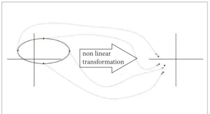
Essentially this is a manner of calculating the statistics of a random variable that passes through a nonlinear transformation. h e UT approach is illustrated in Fig. 1 (Julier and Uhlmann, 1997; van der Merwe, 2004): select a suitable set of points (sigma-points) so that their mean and covariance are x and P xx, respectively (Julier and Uhlmann, 1997, 2004). In turn, the
Figure 1. Unscented transform.
non linear transformation
nonlinear function is applied to each point of the set to yield a cloud of transformed points. h e statistics of the transformed points (mean y and covariance P yy) can then be calculated to form an estimate of the nonlinearly transformed mean and covariance.
h e sigma-points are carefully and deterministically chosen so that they exhibit certain specii c properties, that is, they are not drawn at random like common Monte Carlo methods. Besides, they can be weighted in ways that are inconsistent with the distribution interpretation of sample points like in a particle i lter (Julier and Uhlmann, 1997; van der Merwe, 2004).
he n-dimensional random variable x, with x mean and P xx covariance, is approximated by 2n+1 weighted points, the so known sigma-points, given by:
χi+n = x - (√n+λ) Pxx i χi = x + (√n+λ) Pxx i χ0 = x
(1)
in which λ=α2(n+k)-n includes scaling parameters. h e constant parameter α controls the size of the sigma-points
distribution (0≤α≤1), and k provides an extra degree of
freedom used to i ne-tune the higher order moments; k = 3 -n
for a Gaussian distribution (Wan and van der Merwe, 2001).
In Eq. 1, each element of the n-dimensional random variable
x is replaced by a set of sigma-points generated from the
mean and the covariance of x. h us, the vector variable x has
become a matrix of n x i dimension.
h e transformation occurs as follows:
• Transform each point through the nonlinear function to
yi = f [χi] (2)
• h e observations mean is given by the weighted average
of the transformed points:
y=
∑
Wi yii=0 2n
(3)
• h e covariance is the weighted outer product of the
transformed points:
Pyy=
∑
Wi[yi - y][yi-y] T i=02n
(4)
Wi is the weight associated to the i-th point given by:
W
0 =(n + k)
k
W
i =
2(n + k)
1 , i = 1,..., n
W
i+n =
2(n + k)
1
, i = 1,..., n
(5)
UNSCENTED KALMAN FILTER
Using UT, the following steps are processed in the KF:
• Predict the new state system and its associated covariance,
taking into account the ef ects of the Gaussian white noise process.
• Predict the expected observation and its residual innovation
matrix considering the ef ects of the observation noise.
• Predict the cross correlation matrix.
In order to lead to the new i lter, the UKF, these steps are arranged in the EKF, re-structuring: the dynamics; the state vector; and the observations model.
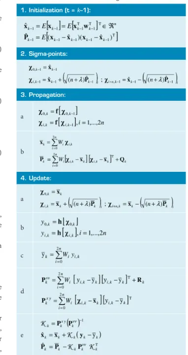
Table 1 presents an algorithm for the UKF. In the i lter
initialization, the mean, x^k-1, and the covariance matrix, P
k-1 ^
, of the state vector x are calculated, in reference to the prior
instant, t k-1. Following, the set of sigma-points is generated,
from the mean and the covariance matrix, previously calculated. In the propagation step, the generated state
sigma-point set is propagated to the instant tk, using the
nonlinear dynamics equation (a), and the predict mean and covariance matrix are calculated (b). During the update cycle: the observations sigma-points are generated (a), propagated through the nonlinear observations equation (b), and its
mean is obtained (c); the predict matrices of innovation, Pkvv,
and correlation, Pkxy
, are computed (d); and i nally the Kalman
gain is calculated, in order to update the state x^k, and the
covariance matrix, P^k. h ey are used as a priori information in
the next instant, tk+1, to generate the new set of sigma-points.
EXTENDED KALMAN FILTER
If the dynamical system and the observations model are linear, the KF is the recursive estimator most used at Table 1. Unscented Kalman i lter algorithm.
1. Initialization (t = k–1):
2. Sigma-points:
3. Propagation:
a
b
4. Update:
a
b
c
d
the present day since it is easy to implement and to use on digital computers. Its recursiveness leads to lesser memory storage, which makes it ideal for real-time applications. he EKF is a nonlinear version of the KF that generates reference trajectories which are updated at each measurement processing, at the corresponding instant (Maybeck, 1982; Brown and Hwang, 1985).
Because it is very diicult to accurately model the artiicial satellites orbit dynamics, the EKF is generally used in works of such nature. Its algorithm always brings updated reference trajectory around the most current available estimate.
Exploiting the assumption that all transformations are quasi-linear, the EKF simply linearizes all nonlinear transformations and substitutes the Jacobian matrices for the linear transformations in the KF equations. he EKF consists of phases of time and measurement updates. In the irst one, state and covariance are propagated from one precedent instant to a posterior one, which means that they are propagated between discrete instants of the system dynamics model. In the second one, state and covariance are corrected from the measurement obtained in the posterior instant of time, through the observations model. herefore, the method nature is recursive, so it does not need to store previously the measurements in large matrices.
Following, the step for the EKF time update (or propagation) cycle is presented:
xk= f(xk-1) ^
Pk= φk,k-1Pk-1φk,k-1 + Qk
^ T .
(6)
where f is a nonlinear vector function modeling the orbit motion,
xk and Pk are respectively the propagated state and the covariance
for tk; φk,k-1 is the state transition matrix between tk-1 e tk; Qk is the
dynamics noise matrix given in Eq. 7. It is required the Jacobian
matrix (∂f/∂x) for the transition matrix computation, which can
be either simpliied or very diicult to obtain.
Qk= ʃt φ(t, tk-1)G(t)Q(t)G
T(t)φT(t, t k-1)dt t
k-1 k
(7)
he equations for the EKF measurement update cycle are:
Kk= PkHk (HkPkHk +Rk)
-1
T T
^
Pk= (I-KkHk) Pk
^
xk= xk + Kk [yk-hk(xk)]
(8)
In Eq. 7, G(t) is the white noise addition matrix. In Eq. 8,
hk is a nonlinear vector function modeling the measurements;
Hk is the corresponding partial derivative matrix ∂hk ∂x ;Kk
is the Kalman gain; Rk is the observations noise matrix; x^k and
P^k are respectively the state vector and the covariance updated
for the instant k; yk is the observations vector corresponding
to the instant k.
Notwithstanding, the EKF has limitations. First: linearization can produce highly unstable ilters if the assumptions of local linearity are violated; second: the derivation of the Jacobian matrices is nontrivial in most applications, and oten leads to signiicant implementations diiculties (Julier and Uhlmann, 1997); third: analytical Jacobian matrices can be a very diicult and error-prone process.
Summarizing, linearization, as applied in the EKF, is widely recognized to be inadequate, but the alternatives incur substantial costs in terms of derivation and computational complexity. Hence, there is a strong need for a method that is probably more accurate than linearization but does not incur costs of implementation and computational of higher order than the other ilters. he sigma-point algorithms were developed to meet these needs (Julier and Uhlmann, 1997).
ORBIT DETERMINATION
The observation may be obtained from the ground station networks using laser, radar, Doppler, or by space navigation systems, as the GPS. The choice of the tracking system depends on a compromise between the goals of the mission and the available tools. In the case of the GPS, the advantages are global coverage, high precision, low cost, and autonomous navigation resources. The GPS may provide orbit determination with accuracy at least as good as methods using ground tracking networks. The later provides standard precision around tens of meters and the former can provide precision as tight as some centimeters. The GPS provides, at a given instant, a set of many redundant measurements, which makes the orbit position observable geometrically.
After some advances of technology, the single frequency GPS receivers provide a good basis to achieve fair precision at relatively low cost, still attaining the accuracy requirements of the mission operation. The GPS allows the receiver to determine its position and time geometrically anywhere at any instant with data from at least four satellites. The principle of navigation by satellites is based in sending signals and data from the GPS satellites to a receiver located onboard the satellite that needs to have its orbit determined. This receiver measures the travel time of the signal and then calculates the distance between the receiver and the GPS satellite. If the clocks are not synchronized, four measurements are required to obtain its position. Those measurements of distances are called pseudo-ranges.
he instantaneous orbit determination using GPS satellites is based on the geometric method. In such method, the observer knows the set of GPS satellites position in a reference frame, obtaining its own position in the same reference frame.
However, sequential orbit determination makes use of the orbital motion modeling to predict between measurement times and measurement model to update the orbit by processing of measurements from GPS. his gives rise to recursive and real-time KF estimator for the orbit determination (Brown and Hwang, 1985).
FILTER DYNAMIC MODEL
In the case of orbit determination via GPS, the ordinary diferential equations which represent the dynamic model are in its simplest form, given traditionally as follows:
r = v
v = -μ r3
r + a + w
v
b = d
d = 0 + w
d .
. . .
(9)
wherein the variables are placed in the inertial reference
frame. In Eq. 9, r is the vector of the position components
(x, y, z); v is the velocity vector; a represents the modeled
perturbing accelerations; w v is the white noise vector with
covariance Q ; b is the user satellite GPS clock bias; d, the user
satellite GPS clock drit; and wd the noise associated with
the GPS clock. he GPS receiver clock ofset was not taken into account, so as not to obscure the conclusions drawn in this paper due to introduction of clock ofset models in the ilters. Indeed, the receiver clock ofset was beforehand obtained and used to correct the GPS measurements, so that the measurements are free from the error derived from receiver clock ofset.
FORCE MODEL
he main disturbing forces of gravitational nature that afect the orbit of an Earth’s artiicial satellite are: the non-uniform distribution of Earth’s mass; ocean and terrestrial tides; and the gravitational attraction of the Sun and the Moon. here are also the non-gravitational efects, such as: Earth atmospheric drag; direct and relected solar radiation pressure; electric drag; emissivity efects; relativistic efects; and meteorites impacts.
he disturbing efects are in general included according to the physical situation presented and to the accuracy that is intended for the orbit determination. Here, we include only a minimum set of perturbations which enable us to assess the performance of both ilters, namely geopotential and third body point mass efect of Sun and Moon.
he Earth is not a perfect sphere with homogeneous mass distribution, and cannot be considered as a material point. Such irregularities disturb the orbit of an artiicial satellite and the keplerian elements that describe the orbit do not behave ideally. he geopotential function can be given by (Kaula, 1966):
∑ ∑
n=0∞ U (r, ϕ, λ)=
r
μ n
m=0 r
RT n
Pnm(sin ϕ)(Cnmcos mλ + Snmsin mλ) (10)
where µ is Earth gravitational constant; RT is mean Earth
latitude; λ is the longitude on Earth ixed coordinates system;
Cnm and Snm are the harmonic spherical coeicients of degree
n and order m; Pnm are the associated Legendre functions. he
constants µ, RT, and the coeicients Cnm, and Snm determine a
particular gravitational potential model.
Another gravitational perturbation source is due to the Sun and Moon attraction. hey are more meaningful at larger distance from Earth. As the orbital variations are of the same type, be the Sun or the Moon the attractive body, they are normally studied without distinguishing the third body. he Sun–Moon gravitational attraction mainly acts on node and perigee, causing precession of the orbit and on the orbital plane. he general three-body problem model is here simpliied to the circular restricted three-body problem, where the orbital motion of a third body (satellite), which mass can be neglected, around two other massive bodies is studied. he force acting on the third body (the satellite) in the inertial reference frame can be expressed as (Prado and Kuga, 2001; Guan, 2013):
r3= -Gm1
r3 r13
-Gm2
13 r
3
r23
23
:
(11)
where r 13 = r 3 - r 1, r 23 = r 3 - r 2, and r i, i=1,2,3 corresponds
to the i-th body distance vector to the center of mass of
the system; and m1 and m2 are the masses of the Sun and the
Moon, respectively.
OBSERVATIONS MODEL
he nonlinear equation of the observation model is:
yk= hk (xk, t) + v
k (12)
where, at time tk, yk is the vector of m observations; hk(xk) is
the nonlinear function of state xk, with dimension m; and vk
is the observations errors vector, with dimension m and
covariance Rk. For the present application, one only uses
the ion-free pseudo-range measurements from the GPS receiver of T/P satellite. Also, the receiver clock offset was computed before and used to correct the pseudo-range measurements. In addition, the nonlinear pseudo-range
measurement was modeled according to Chiaradia et al.
(2003).
MEASUREMENTS SAMPLING
RATES IMPACT IN THE ORBIT
DETERMINATION
Previous presented studies (Pardal et al., 2009b, 2010 and Pardal, 2011) showed that the accuracy improvement for the dynamics models did not better the errors resulting between the references from precise orbit ephemeris from JPL/NASA (POE/JPL) and the values stemming from ilters estimation process. his means that the magnitude of the errors obtained through the UFK or EKF is not reduced when increasing the complexity of the dynamic model: from a model for the geopotential with high degree and order to a complex model containing the three major disruptive efects of the orbit. Further, such results showed an equivalent competitiveness between the estimators, since the errors are of the same order of magnitude. It might have occurred because, in those results, the orbit determination process was done for small sampling intervals of the measurements.
Taking this into account, before concluding that a simpler dynamics modeling can be indiscriminately adopted, there is
a need for another test (Pardal et al., 2010). Such test has two
well determined purposes: to examine carefully the beneits of increasing the adopted dynamics model accuracy; and to investigate the apparent competitiveness between the estimators. his test rested in executing the orbit determination process considering diferent intervals between the GPS observations (pseudo-range) sampling. he intervals of sampling were 10, 30, 60, 300, 600, 1200, and 1800 seconds, in other words, conditions were swept from one very small range (10 seconds) to a range extremely high (1800 seconds) between the prediction and the subsequent correction of the predicted values to complete the cycle of the estimation process. With the gradual spacing of the interval between two measurements, the intention was to verify the dynamics models complexity, and the application of each ilter in the time update cycle. In such situation, the propagation has it efects raised and the modeling accuracy becomes more signiicant in the accuracy of both ilters estimative.
RESULTS
the methods, real GPS data from the T/P satellite are used. he ilters estimated position and velocity are compared with T/P POE from JPL/NASA. he test conditions consider real ion-free pseudo-range data, collected by the GPS receiver onboard T/P, on November 19, 1993, at diferent sampling rates, presenting on average between 5 and 6 GPS satellites tracked. he GPS data were previously preprocessed to remove the outliers so they cannot mislead the ilters or mask diferent data rejection policies of each ilter. he tests have covered a long one day period of orbit determination.
he force model goes from a simple geopotential up to order and degree (2×2), with harmonic coeicients from JGM-2 model, to a model including perturbations due to geopotential up to order and degree (28×28) and due to the
Sun–Moon gravitational attraction (Pardal et al., 2009a, 2010,
2011). he pseudo-range measurements were corrected to the irst order with respect to ionosphere.
As already pointed, this work is not a search for results accuracy. It aims at UKF robustness assessment, which is done through the comparison of performance between UKF and EKF estimators under different sampling rates. There are peculiar interest for speed convergence, and divergence occurrence.
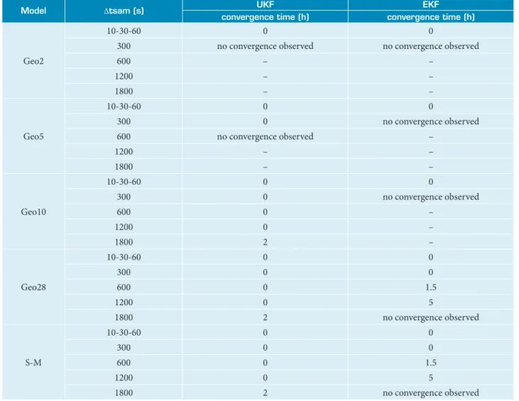
Table 2 shows the analysis for the predicted pseudo-range residuals convergence, which is measured in terms of time span,
Dtsam, of data processed. he convergence is assumed when
the residuals achieve similar statistics of the reference solution residuals. When small samplings intervals, such as 10, 30, and 60 seconds are used, convergence occurs instantaneously ater the estimation process starts, for both UKF and EKF algorithms,
Table 2. Pseudo-range residuals convergence speed.
Model ∆tsam (s) UKF EKF
convergence time (h) convergence time (h)
Geo2
10-30-60 0 0
300 no convergence observed no convergence observed
600 – –
1200 – –
1800 – –
Geo5
10-30-60 0 0
300 0 no convergence observed
600 no convergence observed –
1200 – –
1800 – –
Geo10
10-30-60 0 0
300 0 no convergence observed
600 0 –
1200 0 –
1800 2 –
Geo28
10-30-60 0 0
300 0 0
600 0 1.5
1200 0 5
1800 2 no convergence observed
S-M
10-30-60 0 0
300 0 0
600 0 1.5
1200 0 5
and for any dynamics model adopted. For this reason, results obtained for 10, 30, and 60 seconds of sampling interval will be placed in the same line of Table 1. he model of geopotential up to low order and degree 2×2 (Geo2) starts diverging for 300 seconds of sampling interval, regardless of the estimator applied. he improved geopotential up to order and degree 5×5 (Geo5) dynamics model stops converging when UKF is the ilter for 600 seconds, while EKF is not able to converge at all since 300 seconds. From an improved geopotential model and on, there is always occurrence of divergence when EKF is the algorithm, and convergence keeps occurring if UKF is the chosen algorithm. hat is to say: for geopotential up to order and degree 10×10 (Geo10), divergence is detect at 300 seconds; and for geopotential up to high order and degree 28×28 (Geo28), and for a model that compounds geopotential up to order and degree 28 with Sun-Moon gravitational attraction (S-M), there is occurrence of divergence at 1800 seconds. he convergence time (consequently the convergence speed) is the same for the Geo28
and the S-M models up to 300 seconds of sampling interval, for both estimators, as shown in Table 1. he ilters convergence time starts to be diferent at 600 seconds of interval between two measurements, and this diference keeps the same for each test case (600, 1200, or 1800 seconds), whether the model is Geo28 or S-M. At this point it is possible to pinpoint a model limitation for convergence analysis.
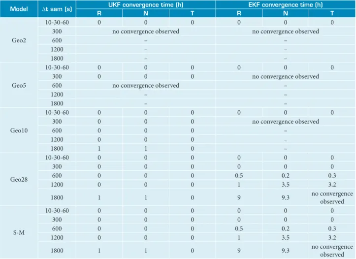
Table 3 shows the convergence analysis for the position RNT (radial, normal, and along-track) components error, which is again measured in terms of data time of processing. When small intervals of sampling are used, such as 10, 30, and 60 seconds, convergence is detected instantaneously ater the starts of the estimation process, for the two estimators, and for any choice of dynamics model. From 300 seconds on, the behavior is the same described in Table 2. he Geo2 model errors start diverging for 300 seconds of sampling interval, regardless of the estimator applied. he improved Geo5 dynamics model errors stop converging when the UKF is the ilter for 600 seconds, while
Table 3. Errors in position convergence speed.
Model ∆t sam (s) UKF convergence time (h) EKF convergence time (h)
R N T R N T
Geo2
10-30-60 0 0 0 0 0 0
300 no convergence observed no convergence observed
600 – –
1200 – –
1800 – –
Geo5
10-30-60 0 0 0 0 0 0
300 0 0 0 no convergence observed
600 no convergence observed –
1200 – –
1800 – –
Geo10
10-30-60 0 0 0 0 0 0
300 0 0 0 no convergence observed
600 0 0 0 –
1200 0 0 0 –
1800 1 1 0 –
Geo28
10-30-60 0 0 0 0 0 0
300 0 0 0 0 0 0
600 0 0 0 0.5 0.2 0.3
1200 0 0 0 1 3.5 3.2
1800 1 1 0 9 9.3 no convergence
observed
S-M
10-30-60 0 0 0 0 0 0
300 0 0 0 0 0 0
600 0 0 0 0.5 0.2 0.3
1200 0 0 0 1 3.5 3.2
1800 1 1 0 9 9.3 no convergence
the EKF is not able to converge at all since 300 seconds. For the Geo10 dynamic model, divergence is detected at 300 seconds; and for the Geo28, and S-M models, there is occurrence of divergence at 1800 seconds. Again, for models Geo28 and S-M, it can be noticed that i lters convergence time dif erence starts at 600 seconds of sampling interval, and this dif erence keeps the same for each test case (600, 1200, or 1800 seconds), no matter the model. So far, a model limitation for convergence analysis might be clear.
Another statistical check is done, in order to coni rm that
the algorithms ef ectively reached convergence. h e reference
pseudo-range residuals statistics (mean and standard deviation) for each model and i lter are available in the yellow lines of Table 4. As the three most improved dynamics models (Geo10, Geo28, and S-M) statistics for 10, 30, and 60 seconds
considerably resemble (Pardal et al., 2009b, 2010), “reference” in
Table 4 refers to a 60-s sampling interval, and is representative of the three intervals. Now, in the analysis of the two poorest dynamics models (Geo2 and Geo5), all the sampling intervals are explicit in Table 4 in order to show poor dynamics behavior as the sampling intervals increase. It is clear that poor dynamics models are more sensitive to the intervals enlargement, since Geo2 model stops converging at 300 seconds, and Geo5, at 300
or 600 seconds, depending on the estimator applied. h rough
Table 4 it is also noticeable that if the model is too poor (e.g., Geo2), neither UKF nor EKF are able to keep convergence for larger sampling intervals, and divergence behavior is detected at 300 seconds for both. However, if the model is slightly improved (for instance, Geo5), UKF implementation shows more robustness than EKF one, because still converges at 300 seconds, while EKF starts diverging. From Table 3, it becomes evident that the estimators really reached convergence, since their statistical values remain nearly the same as the reference ones.
In order to portray such i ndings, Fig. 2 illustrates the reference residuals (small sampling intervals of 60 seconds) behavior, and the 1800 seconds sampling interval case behavior for both the EKF and the UKF estimators, using S-M as the dynamics model. It clearly indicates clues of EKF’s divergence for such larger sampling intervals of measurements.
Proceeding the investigation, Table 5 shows total Root Mean Square (RMS) position error, where the reference values are again listed in the i rst row (yellowed). Again, in the analysis of the two poorest dynamics models (Geo2 and Geo5), all the sampling intervals are registered in Table 5 in order to show poor dynamical behavior as the sampling
Figure 2. Pseudo-range residuals convergence and divergence occurrences.
r e f e r e n c e : U K F - ∆ t s a m = 6 0 s
200
re
si
d
u
al
s
(m
)
150
100
50
0
-50
-100
-150
-200
U K F - ∆ t s a m = 1 8 0 0 s
200
re
si
d
u
al
s
(m
)
150
100
50
0
-50
-100
-150
-200
E K F - ∆ t s a m = 1 8 0 0 s
200
re
si
d
u
al
s
(m
)
150
100
50
0
-50
-100
-150
-200
t i m e ( h)
10 8 6 4 2
0 12 14 16 18 20 22 24
intervals increase. It is clear that poor dynamics models are more responsive to the intervals increasing: the Geo2 model results stop converging at 300 seconds while the Geo5, at 300 or 600 seconds, according to the estimator applied.
h rough Table 5 it is also perceptible that for an excessively
converges at 300 seconds, while EKF starts diverging, which indicates more robustness of UKF when compared to EKF. UKF and EKF resulting RMS errors are only computed at er assumed convergence time. For Table 5, it is also verii able
that the estimators really reached convergence, since their RMS values remain nearly close to the reference ones.
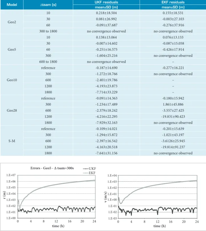
Next, Fig. 3 depicts a particular case where a relatively poor Geo5 dynamics model is adopted. While the UKF i lter
Table 4. Pseudo-range residual statistics, after convergence.
Model ∆tsam (s) UKF residuals EKF residuals
mean±SD (m) mean±SD (m)
Geo2
10 0.218±18.504 0.155±18.531
30 0.081±26.992 -0.003±27.103
60 -0.091±37.687 -0.276±37.916
300 to 1800 no convergence observed no convergence observed
Geo5
10 0.138±13.064 0.076±13.133
30 -0.007±14.602 -0.087±15.058
60 -0.251±16.575 -0.426±17.914
300 -1.604±25.216 no convergence observed
600 to 1800 no convergence observed –
Geo10
reference -0.187±14.690 -0.277±16.221
300 -1.272±18.766 no convergence observed
600 -2.401±19.786 –
1200 -4.193±23.873 –
1800 -7.714±33.229 –
Geo28
reference -0.091±14.363 -0.180±15.942
300 -1.234±17.489 1.861±45.886
600 -2.379±18.242 -3.557±27.425
1200 -4.216±22.295 -19.831±90.423
1800 -7.929±32.163 no convergence observed
S-M
reference -0.109±14.021 -0.201±15.639
300 -1.294±15.872 -1.021±43.197
600 -2.397±16.542 -3.6126±25.945
1200 -4.163±20.518 -19.814±91.237
1800 -7.641±31.156 no convergence observed
Figure 3. Convergence and divergence behavior for Geo5 dynamics model.
Errors - Geo5 - ∆ tsam=300s
1. E + 07
r (m)
1. E + 06
1. E + 05
1. E + 04
1. E + 03
1. E + 02
1. E + 01
1. E + 00
time (h)
8 4
0 12 16 20 24
1.E+04
UKF EKF
v
(m
/s
)
time (h)
8 4
0 12 16 20 24
1. E - 01
1. E - 02
1. E - 03 1. E + 04
1. E + 03
1. E + 02
1. E + 01
remains converging, a divergence behavior is shown in the EKF implementation, for 300 seconds of sampling interval between two measurements. his result indicates that even if the model is not adequately chosen, the EKF believes that the model and linearization are correct. he UKF does not have linearizations and, in adverse situations, such as the ones of larger sampling intervals between two data samples or inaccurate initial
conditions (Pardal et al., 2011), behaves more adequately.
However, if the dynamics model is extremely truncated, such as the Geo2 analyzed in this work, neither the UKF nor the EKF will reach convergence for large sampling intervals, as shown in Tables 1–4. In Fig. 3, ∆r and ∆v represents, respectively, the absolute value of the errors in position and in velocity, in the inertial reference frame coordinates.
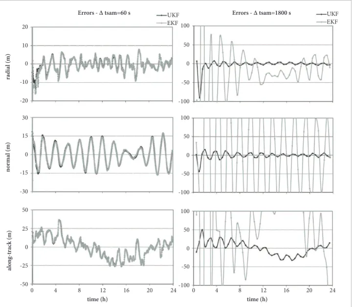
Figure 4 shows the errors in the RNT components for the UKF and EKF reference cases (small 60-s sampling interval, let side) and the larger 1800 seconds error case results for the
EKF and the UKF estimators (right side). he outstanding behavior in the right side happens again in any “no convergence observed” case pointed out in Table 4. It indicates signs of the EKF divergence for such a very large sampling interval, while UKF reaches the convergence zone, not much later than the let side results. So far, the results showed that the performance of the ilters decreases as increasing the sampling intervals (according to assays of the error in position, the pseudorange residuals, and the convergence presented previously). hese results point to the advantage of using the nonlinear theory for orbital dynamics, in small intervals of the UKF and the EKF algorithms.
In order to inish the results analysis, it is to be said that even considering the convergence for small sampling intervals, where UKF and EKF present similar performance, the algorithm is very sensitive to the initialization of the covariance matrix. his means that the algorithm convergence depends on the proper choice of such matrix. herefore, the Table 5. Error in position total Root Mean Square, after convergence.
Model ∆tsam (s) UKF EKF
total RMS(m) total RMS(m)
Geo2
10 34.336 34.391
30 49.834 49.703
60 68.774 69.837
300 to 1800 no convergence observed no convergence observed
Geo5
10 20.521 20.642
30 20.050 20.301
60 22.481 27.303
300 35.562 no convergence observed
600 to 1800 no convergence observed –
Geo10
reference 18.150 23.953
300 22.273 no convergence observed
600 22.658 –
1200 24.000 –
1800 28.962 –
Geo28
reference 17.135 23.159
300 19.217 21.798
600 19.386 29.487
1200 20.943 no convergence observed
1800 26.420 –
S-M
reference 16.253 22.520
300 15.437 18.416
600 15.398 26.489
1200 16.403 no convergence observed
30
n
o
rma
l (m)
15
100
50
0
-50
-100 -15
-30
0
time (h)
50
al
o
n
g-tr
ac
k (m)
25
100
50
0
-50
-100 -25
-50
time (h)
8 4
0 12 16 20 24 0 4 8 12 16 20 24
0
Figure 4. Convergence and divergence behavior of the errors in RNT (radial, normal, and along-track) components. Errors - ∆ tsam=60 s
20
radi
al (m)
10
100
50
0
-50
-100 -10
-20
Errors - ∆ tsam=1800 s
UKF EKF
UKF EKF
0
results are not general, and the algorithm was adjusted for this type of orbit determination application.
CONCLUSIONS
h e robustness to increasing sampling intervals of two
nonlinear estimators, namely the EKF and UKF was assessed for a real-time satellite orbit determination problem using real GPS measurements. One day (24h) of GPS receiver measurements of T/P satellite at dif erent sampling rates
were processed. h e emphasis was to characterize each i lter
convergence behavior in situations where the sampling rates vary from small to larger intervals between two measurements. Dif erent dynamical models were analyzed, in order to establish the modeling ef ects in the orbit determination process.
Results showed that when small sampling intervals are used, UKF and EKF yield similar performance, with high
performance, for almost all dynamics models. h e exception
REFERENCES
Brown, R. G. and Hwang, P. Y. C., 1984, A Kalman ilter approach to precision GPS geodesy, Navigation: Global Positioning System, Vol. II, pp. 155-166.
Brown, R. G. and Hwang, P. Y. C., 1985, Introduction to random signals and applied Kalman iltering, 3rd ed. New York: John Wiley & Sons. 502 p.
Chiaradia, A. P. M., Kuga, H. K. Kuga and Prado, A. F. B. A., 2003, Single frequency GPS measurements in real-time artiicial satellite orbit determination, Acta Astronautica, Vol. 53, n. 2, pp. 123-133.
El-Sheimy, N., Shin, E-H. and Niu, X., 2006, Extended vs. Unscented Kalman Filters for Integrated GPS and MEMS Inertial. Available from: http://www.insidegnss.com/auto/0306%20Kalman.pdf
Guan, T., 2013, Special cases of the three body problem, [online Colorado University database]. Available from: http://inside.mines.edu/ fs_home/tohno/teaching/PH505_2011/Paper_TianyuanGuan.pdf
Jose, J. M., 2009, Performance comparison of Extended and Unscented Kalman Filter implementation in INS-GPS integration, Ph.D thesis. Czech Technical University in Prague, Prague (in English). Available from: http://epubl.ltu.se/1653-0187/2009/095/LTU-PB-EX-09095-SE.pdf
Julier, S. J. and Uhlmann, J. K., 1997, A new extension of the Kalman ilter for nonlinear systems, International Symposium on Aerospace/ Defense Sensing, Simulation and Controls. SPIE.
Julier, S. J.and Uhlmann, J. K., 2004, Unscented iltering and nonlinear estimation. IEEE Transactions on Automatic Control, Vol. 92, n. 3, Mar 2004.
Kaula, W.M., 1966, Theory of Satellite Geodesy. Blasdell Pub. Co. Walthmam, Mass.
Maybeck, P.S., 1982, Stochastic models, estimation, and control. Vol. 2, Academic Press, NY.
Montenbruck, O. and Gill, E., 2001, Satellite orbits: models, methods, and applications, Springer-Verlag, Berlin Heidelberg NewYork. 369 p.
Pardal, P. C. P. M., Kuga, H. K. and Vilhena de Moraes, R., 2009a, A discussion related to orbit determination using nonlinear sigma point Kalman ilter, Mathematical Problems in Engineering, v. 2009, 12 p. Hindawi Publishing Corporation, doi:10.1155/2009/140963.
Pardal, P. C. P. M., Kuga, H. K. and Vilhena de Moraes, R., 2009b, Non linear sigma point Kalman ilter applied to orbit determination using GPS measurements, 22nd International Meeting of the Satellite Division of the Institute of Navigation (ION GNSS 2009), 22–25 Sept., Savannah, USA.
Pardal, P. C. P. M., Kuga, H. K. and Vilhena de Moraes, R., 2010, Comparing the extended and the sigma point Kalman ilters for orbit determination modeling using GPS measurements,23rd International Meeting of the Satellite Division of the Institute of Navigation (ION GNSS 2010), 21-24 Sept., Portland, USA.
Pardal, P. C. P. M., Real time orbit determination through non linear sigma-point Kalman ilter, 2011, Ph.D thesis, National Institute for Space Research (INPE), São José dos Campos. (In Portuguese).
Pardal, P. C. P. M., Kuga, H. K.and Vilhena de Moraes, R., 2011, Robustness assessment between sigma point and extended Kalman ilter for orbit determination,. Journal of Aerospace Engineering, Sciences and Applications, v. III, pp. 35-44. doi: 10.7446/ jaesa.0303.04
Prado, A. F. B. A. and Kuga, H. K. (Eds.), 2001, Space Technology Fundaments, São José dos Campos: INPE. 220 p. (In Portuguese).
Soken, H. E. and Hajiyev, C., 2011, REKF and RUKF Development for Pico Satellite Attitude Estimation in the Presence of Measurement Faults, 5th International Conference on Recent Advances in Space Technologies (RAST), 9–11 June 2011. pp. 891-896. doi: 10.1109/ RAST.2011.5966972
van der Merwe, R., 2004, Sigma-Point Kalman ilters for probabilistic inference in dynamic state-space models, Ph.D thesis. Oregon Health & Science University, Portland.
van der Merwe, R., Wan, E.A. and Julier, S.J., 2004, Sigma-point Kalman ilters for nonlinear estimation and sensor-fusion applications to integrated navigation, AIAA Guidance, Navigation, and Control Conference and Exhibit, 16-19 Aug. 2004, Rhode Island.
Wan, E. A. and van der Merwe, R., 2001, The unscented Kalman ilter, Kalman Filtering and Neural Networks. Haykins, S. (Ed.), John Wiley & Sons, New York, Chap. 7.
ilters performance. As larger is the interval more diicult is for EKF and UKF to reach convergence. When UKF is compared with EKF, in all cases of larger intervals, the UKF always attains convergence irst. he rupture threshold for this application in particular occurs to all modeling complexities if EKF was the used algorithm. Only in two situations (the two poorest models adoption) for the UKF implementation, divergence occurred. herefore it is to be said that the UKF is more robust than the EKF for larger sampling interval between measurements, for this type of orbit determination application.