KJMA theory is useful even when nucleation and growth retain solely an operational meaning.
In a recent work, Rios and Villa14 resorted to recent developments on stochastic geometry15-17 to revisit the classical KJMA theory and generalize it for situations in which nucleation took place both for homogeneous and for inhomogeneous Poisson point processes. “Nuclei being located in space according to a homogeneous Poisson point process” simply means that they are uniform randomly located in space. Poisson point processes will be more rigorously defined in section 2 below.
For that matter, VV and VE were replaced by a position-dependent mean volume density, VV(t, x), mean extended volume density
VE (t, x), where x = (x1, x2, x3) is the spatial coordinate. Thus, the relationship between volume fraction and extended volume fraction, Equation 1, became a relationship between the mean volume density and the mean extended volume density:
VV
( )
t x, = −1 exp(
−VE( )
t x,)
(4) Using this methodology, it was possible to significantly broaden the scope of analytical solutions available. One example of the results obtained by Rios and Villa is an equation for site-saturated nucleation, which closely parallels Equation 3,VV
( )
t x, = −exp− ( )x G t
1 4
3
3 3
πλ (5)
where λ(x) is called the intensity of the inhomogeneous Poisson point process. For Equation 5 to be valid λ(x) must be a harmonic func-tion, i.e must satisfy Laplace’s partial differential equation. For the particular case of uniform randomly located nuclei or synonymously nuclei located according to a homogeneous Poisson point process the intensity is independent of the position and coincides with the
*e-mail: [email protected]
Inhomogeneous Poisson Point Process Nucleation: Comparison
of Analytical Solution with Cellular Automata Simulation
Paulo Rangel Riosa*, Douglas Jardima, Weslley Luiz da Silva Assisa,
Tatiana Caneda Salazara, Elena Villab
a
Escola de Engenharia Industrial Metalúrgica de Volta Redonda,
Universidade Federal Fluminense,
Av. dos Trabalhadores, 420, 27255-125 Volta Redonda - RJ, Brasil
b
Department of Mathematics, University of Milan, via Saldini 50, 20133 Milano, Italy
Received: April 10, 2009; Revised: May 6, 2009
Microstructural evolution in three dimensions of nucleation and growth transformations is simulated by means of cellular automata (CA). In the simulation, nuclei are located in space according to a heterogeneous Poisson point processes. The simulation is compared with exact analytical solution recently obtained by Rios and Villa supposing that the intensity is a harmonic function of the spatial coordinate. The simulated data gives very good agreement with the analytical solution provided that the correct shape factor for the growing CA grains is used. This good agreement is auspicious because the analytical expressions were derived and thus are exact only if the shape of the growing regions is spherical.
Keywords: microstructure, analytical methods, phase transformations, recrystallization, cellular automata
1. Introduction
Transformation kinetics is often described by an expression of the form:
VV
( )
t = −1 exp(−ktn) (1)where, VV is the volume fraction, t is time, k and n are adjustable parameters. Equation 1 is often called “Avrami” equation. In fact, the use of adjustable parameters is in some sense the opposite that Kolmogorov1, Johnson-Mehl2 and Avrami3-5 (KJMA) did. KJMA obtained an exact solution to the problem of nucleation and growth of a new phase. Their solution is not general. They assumed uniform randomly nucleation, either site-saturated or to taking place with a constant nucleation rate. Site-saturated nucleation implies that all nucleation sites are exhausted early in the transformation, or more informally, all nuclei are already present at the time origin, t = 0. Moreover, they further assumed the growth rate, G, to be constant and the growing regions to have a spherical shape. They solved the problem of impingement and obtained an exact expression connecting VV to the extended volume fraction, VE
VV= −1 exp(−VE) (2)
Specifically, their exact analytical expressions for site-saturated nucleation is the well-known expression:
VV= − −
1 4
3
3 3
exp πN G tV (3)
where NV is the number of nuclei per unit of volume.
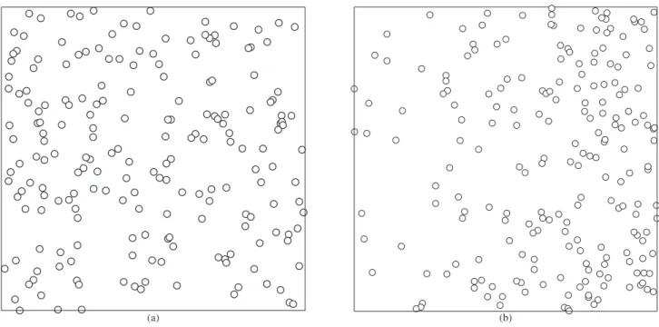
implies time dependence. In fact Figure 1a and 1b represent site-saturated nucleation, or, informally, the situation in which all nuclei are already present at t = 0. Figure 1a depicts nuclei located in what may be intuitively described as “randomly” or uniform randomly. Conversely in Figure 1b the number of nuclei changes from x1 = 0 to
x1 = 1, x1-horizontal axis, following λ(x) = 350 x1 + 25. Therefore, in this case, as x1 changes from 0 to 1 the number of nuclei increases.
More generally, when A is a 3-d region, N(A), is the random number of points/nuclei located within A. If these are Poissonian distributed:
P N A k x
k x
k
( ) ( )
! exp( ( )) =
(
)
=λ −λ (6)where, P (N(A) = k) is the probability of k nuclei falling within the unit volume A and λ(x) is the intensity. In the homogeneous case, the intensity is independent of the spatial coordinate, x. In contrast, in the inhomogeneous case the intensity does depend on the spatial coordinate, λ(x).λ(x) can be interpreted as the mean number of nuclei in the infinitesimal volume dx. Notice that in the homogeneous case λ is constant; therefore in such a case it represents the mean number of nuclei per unit of volume.
For the volume transformed originating from grains that grow from heterogeneously located nuclei, one cannot talk of a volume fraction as was done above. It is necessary to define a mean volume
density, which takes different values depending on x: VV (t, x) and
VE (t, x) corresponding to VV (t) and VE (t), respectively. Of course, one can still find the volume fraction by integration of the mean volume density but now it depends on where the integration volume is located within the specimen. Notice that for a “homogeneous speci-men” the volume fraction, VV (t), represents the probability that an arbitrary point will be transformed regardless of the location of this point in space. For a “heterogeneous specimen” this probability, the mean volume density, VV (t,x), depends on the spatial coordinates
of the point considered. number of nuclei per unit of volume. Further distinction between
homogeneous and inhomogeneous Poisson point process and the definition of VV (t, x) and VE (t, x) are clarified in the Mathematical background section below.
In previous papers18-24, cellular automata (CA) simulation of phase transformation/recrystallization in 2-d and 3-d were carried out and compared with KJMA analytical solutions. The purpose of the present paper is to simulate phase transformations/recrystallization in by cellular automata (CA) in order to compare the simulation with the analytical solution by Rios and Villa. The simulation is restricted to site-saturated inhomogeneous Poisson point process nucleation with the intensity, λ(x), varying linearly along the x1 coordinate but remaining constant for x2 and x3. In order to make such a comparison feasible it is necessary to adapt Equation 5, derived for spherical growth, to CA where growth is not spherical.
Thus, this work presents not only a comparison but in fact it shows that it is possible to use Equation 5 to describe CA even though Equation 5 is not exact for CA, as will become clear in what follows.
Noteworthy, to our best knowledge, this is the first time a com-puter simulation is carried out in which nuclei are located in space according to an inhomogeneous Poisson process.
2. Mathematical Background
A rigorous definition of VV (t, x) and of point processes entail a minimum background in stochastic geometry. Nonetheless, for the present work an intuitive notion of those suffices. Such may be apprehended from Figure 1a and 1b, in which a homogeneous and an inhomogeneous Poisson point process were simulated with the help of the “R” software27. Details that are more mathematical can be found in Rios and Villa14.
Figure 1a and 1b show nuclei, i.e. points, represented by small cir-cles located according to a homogeneous and a heterogeneous Poisson point process, respectively. The word “process” does not necessarily
3. Description of the Cellular Automata Simulation
Cellular automata simulation used a 3-d von Neumann neighborhood26,27. The matrix consisted of a cubic lattice with 300 x 300 x 300 cells. One cell edge was considered to have a length equal to 1/300 so that the simulated domain is effectively a unit cube: [0,1] x [0,1] x [0,1]. Units of all quantities reported here follow from this. Site saturated nucleation was assumed. The nuclei were located in the matrix according to an inhomogeneous Poisson point process with an intensity equal to λ(x) = λ(x1, x2, x3) = 596 x1 + 2. Consequently, 300 nuclei were present at the simulated volume.
The simulation produced a sequence of matrices as a function of time. Time is discrete in CA, it takes integer values starting from
t = 0. One time unit corresponds to the interval between two consecu-tive matrix updates26,27. From the simulated matrices, all the desired quantities could be extracted.
4. Analytical Expressions
4.1. Exact solutions for spherical growth
The exact analytical solutions from Rios and Villa14 for site-saturated nucleation according to an inhomogeneous Poisson process and constant growth velocity, G, are repeated here for convenience. Notice that in what follows α = π.
VV( , )t x = −1 exp(−4 ( )x G t ) 3
3 3
αλ
(7)
and
SV( , )t x =12 ( )x G t exp(−4 ( )x G t ) 3
2 2 3 3
αλ αλ (8)
SV (t, x) is the mean interfacial area density between the new phase and the parent matrix. The microstructural path is:
S t x x V t x
V t x
V V
V
( , ) ( ) ( , ) ln
( , ) =
(
)
(
−)
− 3 36 1 1
1
1 3
2
αλ 33
(9)
If
λ( )x =mx1+n (10)
and supposing λ(x) > 0 and that x belongs to the unit cube, A = [0,1] x
[0,1] x [0,1] ≡ [0,1]3, then using Equation 7.
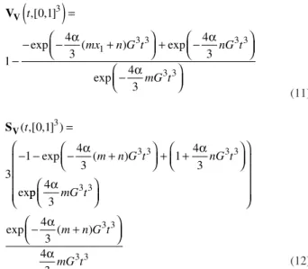
VV t
mx n G t nG t
,[ , ]
exp ( ) exp
0 1 1 4 3 4 3 3
1 3 3 3 3
(
)
=−− − +
α + − α − exp 4 3 3 3 α mG t (11)
SV( ,[ , ] )
exp ( )
ex t
m n G t nG t
0 1 3 1 4 3 1 4 3 3
3 3 3 3
=
− − − α + + + α
p p
exp ( )
4 3 4 3 4 3 3 3 3 3 3 3 α α α mG t
m n G t mG t − + (12)
Moreover, the growth velocity can be obtained from:
G S dV dt S dV dt d dt E E V V
= 1 = 1 = 1
S V
V V
(13)
The relationship between mean and extended mean area density,
SE(t,x) is:
SV( , )t x = −
(
1 VV( , )t x S)
E( , )t x(14)
but
SV( )t ≠ −
(
1 VV( )t)
SE( )t(15)
It is worthy pointing out again that for all the equations in this subsection α= π.
4.2. Analytical expressions for cellular automata
Two important assumptions were made by Rios and Villa14 in the derivation of the above relationships:
a) The growing regions are spherical
b) λ(x) is an harmonic function. In fact, these assumptions may be relaxed14 but in this case V
V (t, x) would not have the simple
form shown in Equations 8-10.
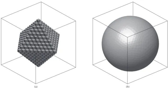
Unfortunately, CA grains are not spherical. The shape of CA is compared with a sphere in Figure 2. The analytical expression equivalent to Equation 3 for CA was derived by Rios et al.22.
VV = −1 − N G tV 4 3
3 3
exp( )
(16)
Comparison between Equations 3 and 16 shows that a factor of π is "missing" from Equation 16. It is suggested here that, by analogy, one may obtain simple approximate analytical expressions to CA from Equations 7-9 and Equations 11-14, replacing α= π by α= 1. May be, in fact, this is it is not a matter of shape factor α itself, but of the volume of the growing grains. It is as if the theorem for harmonic functions (which holds for spheres) used by Rios and Villa14 in the derivation of Equation 7 holds also for growing grains such as the one depicted in Figure 2a. Strict mathematical proof of this cannot be given at this time.
Thus, Equations 7-9 and 11-14 with α= 1 are compared with the CA simulation in the next section.
5. Results and Discussion
In this section, the expressions derived in the previous section for single grain evolution are compared with CA simulation.
First, it is interesting to show the microstructure resulting from the simulation. Figure 3 depicts a 3-d view of the simulated micro-structures for a) VV = 0; b) VV = 0.1; c) VV = 0.5 and d) VV = 1. The grains are slightly elongated towards the lower plane, x1 = 0. This is more apparent for values of x1 < 0.5. Figure 4 complements Figure 3. It displays the microstructure of the fully transformed specimens of cross-sections taken at planes x1 = 0.1, x1 = 0.5 and x1 = 0.9. It is clear that, as expected, the grain size decreases as the nuclei intensity increases from x1 = 0.1 to x1 = 0.9.
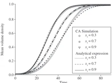
Figure 5 exhibits the volume fraction, the mean volume density,
VV (t, x) as a function of time at planes x1 = 0.3, 0.5, and 0.9. It is worth mentioning that for nuclei too close to x1 = 0 or x1 = 1 one has to use expressions that take into account the influence of the specimen surface given by Rios and Villa14. Figure 6 shows V
good agreement is obtained but a small deviation can be observed for VV close to 1.
A significant change occurred in the way phase transformations have been studied. Formerly, one had to rely on experiments dealing almost exclusively with measurements on 2-d single planar sections. Those experiments were then modeled by theories that were devel-oped bearing in mind the availability of 2-d quantities such as the volume fraction and interfacial area per unit of volume. Moreover, using 2-d sections it is very difficult to detect departures of nucleation from the usual uniform randomly assumption. This is so because the number of nuclei per unit of volume and the non-uniform randomly
located nuclei are inherently 3-d properties. Considerable change took place in recent years with the advent of 3-d computer simulation, such as that carried out here, and 3-d experimental techniques like serial sectioning coupled with computer reconstruction. With such tech-niques, it is now possible to measure and simulate 3-d microstructures. Now, intrinsic 3-d quantities like number of nuclei per unit of volume or even the position of nuclei in space may be measured/simulated. Nonetheless, this advance has not yet been matched by the develop-ment of 3-d analytical treatdevelop-ments such as that put forward by Rios and Villa14. All three approaches, i. e. experimental, simulation and analytical, must converge if one is to have full 3-d understanding of
Figure 2. Comparison between the shape of a growing region in cellular automata, (a), and spherical growth, (b).
the problems. Therefore, the current result is of particular importance as it shows that 3-d analytical and 3-d simulation may be combined to analyze an eventual 3-d experimental dataset of nucleation and growth transformations. Noteworthy, 3-d experimental techniques are very demanding in terms of equipment and labor and therefore it is of considerable interest to gather all possible knowledge of the problem by analytical or computer simulation prior to the experiments itself. Thus, one should not see the theoretical approach just as an useful “after the fact” calculation. On the contrary, these techniques may be pro-actively used from the onset to plan experiments and perhaps locate the experimental range within which it might be more profit-able to invest time and effort.
6. Summary and Conclusions
CA simulation showed very good agreement with exact math-ematical expressions proposed by Rios and Villa even though the shape of CA growing grains is not spherical. However, this good agreement can only be obtained if the appropriate shape factor is
Figure 7. Microstructural path: area of the interface between transformed and untransformed regions per unit of volume, SV, against volume fraction, VV. There is good agreement between theory and simulation.
Figure 4. Fully transformed microstructure on cross-sections taken at planes a) x1 = 0.1; b) x1 = 0.5; and c) x1 = 0.9.
Figure 5. Mean volume density, VV (t, x) as a function of time at planes
x1 = 0.03, 0.5, and 0.9.
used, namely, α = 1 (CA shape) instead of α = π (spherical shape) in Equations 7-12. It is worth mentioning that a full derivation and discussion of the shape factor, α= 1, was carried out in a previous work21.
Acknowledgements
This work was supported by Conselho Nacional de Desenvolvi-mento Científico e Tecnológico, CNPq, Coordenação de Aperfeiçoa-mento de Pessoal de Nível Superior, CAPES, and Fundação de Amparo à Pesquisa do Estado do Rio de Janeiro, FAPERJ.
References
1. Kolmogorov NA. The statistics of crystal growth in metals. Isvestiia Academii Nauk SSSR - Seriia Matematicheskaia. 1937; 1:333-359. 2. Johnson WA, Mehl RF. Reaction kinetics in processes of nucleation and
growth. Transactions AIME. 1939; 135:416-441.
3. Avrami MJ. Kinetics of phase change I general theory. The Journal of Chemical Physics. 1939; 7(12):1103-1112.
4. Avrami MJ. Kinetics of phase change II transformation-time relations for random distribution of nuclei. The Journal of Chemical Physics. 1940; 8(2):214-224.
5. Avrami MJ. Kinetics of phase change III granulation, phase change, and microstructure kinetics of phase change. The Journal of Chemical Physics. 1941; 9(2):177-184.
6. Cahn JW. The kinetics of grain boundary nucleated reactions. Acta Metallurgica. 1956; 4(9):449-459.
7. Vandermeer RA, Masumura RA, Rath B. Microstructural paths of shape-preserved nucleation and growth transformations. Acta Metallurgica et Materialia. 1991; 39(3):383-389.
8. Vandermeer RA, Jensen DJ. Microstructural path and temperature dependence of recrystallization in commercial aluminum. Acta Materialia. 2001; 49(11):2083-2094.
9. Rios PR, Yamamoto T, Kondo T, Sakuma T. Abnormal grain growth kinetics in BaTiO3 with an excess TiO2. Acta Materialia. 2001;
46(5):1617-1623.
10. Yamamoto T, Sakuma T, Rios PR. Application of microstructural path analysis to abnormal grain growth of BaTiO3 with an excess TiO2. Scripta
Materialia. 1998; 39(12):1713-1717.
11. Rios PR, Guimarães JRC. Microstructural path analysis of athermal martensite. Scripta Materialia. 2007; 57(12):1105-1108.
12. Rios PR, Guimarães JRC. Formal analysis of isothermal martensite spread. Materials Research. 2008; 11(1):103-108.
13. Burger M, Capasso V, Salani CV. Modelling multi-dimensional crystallization of polymers in interaction with heat transfer. Nonlinear Analysis - Series B. 2002; 3(1):139-160.
14. Rios PR, Villa E. Transformation kinetics for inhomogeneous nucleation.
Acta Materialia. 2009; 57(11):1119-1208.
15. Stoyan D, Kendall WS, Mecke J. Stochastic Geometry and its Application. 2 ed. Chichester: Wiley; 1995.
16. Capasso V, Villa E. On the evolution equations of mean geometric densities for a class of space and time inhomogeneous stochastic birth-and-growth processes. In: W. Weil, editor. Stochastic Geometry, Lecture Notes in Mathematics. Heidelberg: Springer; 2007. p. 267-281. 17. Villa E. A note on mean volume and surface densities for a class of
birth-and-growth stochastic processes. International Journal Contemporary Mathematical Science. 2008; 3(21-24):1141-1155.
18. Rios PR, Carvalho JJS, Salazar TC, Paula FVL, Castro JA. Cellular automata simulation of the effect of nuclei distribution on the recrystallization kinetics.
Materials Science Forum. 2004; 467-470:659-664.
19. Rios PR, Oliveira JCPT, Oliveira VT, Castro JA. Comparison of analytical models with cellular automata simulation of recrystallization in two dimensions. Materials Research. 2005; 8(3):341-345.
20. Rios PR, Oliveira JCPT, Oliveira VT, Castro JA. Microstructural descriptors and cellular automata simulation of the effects of non-random nuclei location on recrystallization in two dimensions. Materials Research. 2006; 9(2):165-170.
21. Rios PR, Pereira LO, Oliveira VT, Pereira MR, Castro JA. Cellular automata simulation of site-saturated and constant nucleation rate transformations in three dimensions. Materials Research. 2006; 9(2):223-230.
22. Rios PR, Pereira LO, Assis WLS, Oliveira FF, Oliveira VT. Analysis of transformations nucleated on non-random sites simulated by cellular automata in three dimensions. Materials Research. 2007; 10(2):141-146. 23. Rios PR, Pereira LO, Oliveira FF, Assis WLS, Castro JA. Impingement
function for nucleation on non-random sites. Acta Materialia. 2007; 55(13):4339-4348.
24. Salazar TC, Assis WLS, Rios PR. Cellular automata simulation in three dimensions of recrystallization in an iron single crystal. Materials Research. 2008; 11(1):109-115.
25. Hesselbarth HW, Göbel IR. Simulation of recrystallization by cellular automata. Acta Metallurgica et Materialia. 1991; 39(9):2135-2143. 26. Marx V, Reher FR, Gottstein G. Simulation of primary recrystallization
using a modified three-dimensional cellular automaton. Acta Materialia. 1999; 47(4):1219-1230.