Analytical Solutions of Viscoelastic Flow through Porous Channels

Analytical Solutions of Viscoelastic Flow through Porous

Channels

GHULAM QADIR MEMON*, MUHAMMAD ANWAR SOLANGI** AND AHSANULLAH BALOCH***

RECEIVED ON 16.11.2009 ACCEPTED ON 21.06.2012

ABSTRACT

Viscoelastic flow in channel having transient hydrodynamic behavior, filled with and without porous medium is addressed. The boundary value problem is investigated through analytical and numerical solutions, for the governing system of partial differential equations, arising in the study for flow of viscoelastic fluids. Analytical solutions in terms of velocity, normal stress and shear stress at different values of time, viscosity and Darcy's number are obtained for constant viscosity Oldroyd-B constitutive model. Lie group technique is adopted to find solutions through symmetry of differential equations, whilst numerical solutions are realized by employing ND Solve, Mathematica Solver. Lie group technique is compared against numerical solutions by employing ND Solve, Mathematica Solver. The analytical solutions are observed in good agreement with the numerical solutions.

Key Words: Lie Group Method, Viscoelastic Flow, Porous Media, Exact Solution.

* Assistant Professor, Department of Mathematics, Shah Abdul Latif University, Khairpur Mirs.

* * Assistant Professor, Department of Basic Sciences & Related Studies, Mehran University of Engineering & Technology, Jamshoro. *** Professor, Department of Basic Sciences & Related Studies, Mehran University of Engineering & Technology, Jamshoro.

1. INTRODUCTION

The investigation is addressed in terms of analytical and

numerical solutions of a boundary value problem for

governing system of partial differential equations arising

in the study of the flow of viscoelastic fluids through non

porous and porous medium obeying the constant viscosity

Oldroyd-B constitutive model. The analytical solutions

are obtained by applying Lie group techniques, while

numerical predictions are made by ND- Solve determined

by Mathematica [10-11].

Symmetry group analysis based on the transformation

groups known as Lie groups is most important solution

technique for solving the differential equations and

symmetries can be found to simplify the problem. Lie group

V

iscoelastic fluid flow through porous channels is termed as of practical interest in many investigations, which during deformation illustrate the mixture of both viscous and elastic components [1-5]. Such materials may include toothpaste, paint, blood, oil, cookie dough, soap solutions, cosmetic and etc.

approach is widely applied solving the PDEs, in various

fields of applied mathematics, mechanics and engineering

science.

Symmetries of a differential equations form a

one-parameter group of transformations in which one-parameter

is small and guide to the reduction of the number of

independent variables, has been initiated and developed

in [12]. A theory presented in [13] guide to the

developments in the Lie group method over previous

methods. Some important studies dealing with

development of the Lie group theory is made by a number

of researchers [14-26].

2.

PROBLEM FORMULATION

Consider the incompressible laminar flow of viscoelastic

fluid in a channel filled with porous medium. The system

of governing equations of flow comprises of the

conservation of mass and conservation of momentum

transport coupled with the Oldroyd-B constitutive model.

The flow of viscoelastic fluids through porous media is

assumed to be isotropic and homogeneous. The

momentum equation can be modelled by using

Darcy-Brinkman model and in the absence of body force,

equations of continuity and momentum may be written in

the following form:

Δ.u = 0 (1)

u K u u p d

t

u μ

ρ τ

μ ε ε ρ

− ∇ − ∇ − + ∇

= ∂ ∂

. )

] 2 2 [ ( 1

(2)

The Oldroyd-B constitutive equation describes the viscoelastic stresses in the flow can be expressed as below:

} . ) ( . .

{ ] 1 2

[ μ τ λ τ τ τ

τ

λ T

u u u

d

t = − − ∇ −∇ − ∇

∂ ∂

(3)

In the above equations, u is the velocity vector field of

flow, τ is the extra stress tensor, dis the rate-of-strain tensor, Δ is the spatial differential operator, p is the isotropic fluid pressure (per unit density) and t is the time. The μ₁ and μ₂ are respectively the viscoelastic solute and Newtonian solvent viscosities, fluid density is denoted

by ρ, whereas λ is the relaxation time of the viscoelastic fluid and K is the intrinsic permeability of the porous

medium. Total viscosity μ of the viscoelastic flow is μ=μ₁

+μ

2 and is taken constant. The acceleration coefficient

tensor (ε) in Equation (2) is assumed as porosity of porous media.

The equations are derived which govern the unsteady

unidirectional flow of viscoelastic fluid through porous

media adopting Oldroyd-B constitutive model. The

derivation of such equations by employing the momentum

transport equation of viscoelastic fluid and Oldroyd-B

constitutive equations assuming constant pressure

gradient and may be expressed in the absence of body

force as follows:

⎪

⎪

⎪

⎭

⎪

⎪

⎪

⎬

⎫

− ∂ ∂ = ∂ ∂

− ∂ ∂ =

∂ ∂

− ∂ ∂ − ∂ ∂ + ∂ ∂ = ∂ ∂

12 1

12

11 12

2 11

12 1 2 2 2

τ μ τ λ

τ τ

λ τ λ

μ τ

ε ε

μ ε

ρ

y v

t

y v

t

v K x p

y y

v

t v

(4)

Where v(y,t) is the velocity component in axial direction and τ₁₁(y,t), τ₁₂(y,t) and τ₂₂(y,t) are the stress tensor components in axial, shear and transversal direction. As y is in the transversal direction where second normal stress vanishes (τ₂₂= 0).

Analytical Solutions of Viscoelastic Flow through Porous Channels

v = v* _V

c, τ=μ Vcτ

*_{/L,y = y}*_{L, K=K}* _{and t=t}*_{L/Vc, along}

with material parameters: λ=λ*_L/Vc, μ 1= μ μ1

*_, μ 2 = μ μ2

*_,

Re= ρLVc /μ.

Where v*_, τ* _{and y}* _{are dimensionless velocity, stress}

tensor and transversal coordinates and t*_{and K}* _{are the}

non-dimensional time and the non-dimensional modified

permeability of the porous medium. Whilst, L is the

characteristic length taken as half width of the channel

and Vc is the characteristic velocity assumed as reference

axial velocity Vc=εL2_(-∂_p/∂_x)/μ_{, then after dropping asterisk}

from variables for brevity, the non-dimensional equations

become:

⎪

⎪

⎪

⎭

⎪

⎪

⎪

⎬

⎫

− ∂ ∂ = ∂ ∂ − ∂ ∂ = ∂ ∂ − ∂ ∂ + ∂ ∂ + = ∂ ∂ 12 1 12 11 12 2 11 1 12 2 2 2 1 Re τ μ τ τ τ τ τ μ y v t We y v We t We v Da y y v t v (5)

Where the dimensionless Re (Reynolds Number), We (Weissenberg Number) and Da (Darcy's Number) are defined as Re=ρLVc /μ, We=λ*₌λ_{Vc /L and Da=K/}ε_L2

respectively.

To complete the well posed problem specification, it is necessary to prescribe initial and boundary conditions.

Here initial conditions are taken from rest i.e.

v (0,y) = 0 when y>0 (6)

and boundary conditions are taken as:

v(t,-1) = 0 and v(t,1) = 0, when t>0 (7)

3.

SOLUTION OF VISCOELASTIC

FLOW THROUGH CHANNEL

WITHOUT POROUS MEDIA

As Da approaches to infinity, the last Darcy's term vanishes, then the system Equation (5) written as:

⎪

⎪

⎪

⎭

⎪

⎪

⎪

⎬

⎫

− ∂ ∂ = ∂ ∂ − ∂ ∂ = ∂ ∂ ∂ ∂ + ∂ ∂ + = ∂ ∂ 12 1 12 11 12 2 11 12 2 2 2 1 Re τ μ τ τ τ τ τ μ y v t We y v We t We y y v t v (8)

Subject to same initial and boundary conditions as referred in Equations (6-7).

3.1

Symmetry Analysis

Once symmetry Lie algebra of the differential equation is known, it can be used in the investigation of transformations that will reduce the equation to simpler form and it is powerful method in obtaining analytical solutions of differential equations. In this section, symmetry conditions and method for finding the Lie point symmetries are introduced.

The Operator: ⎪ ⎪ ⎪ ⎪ ⎭ ⎪⎪ ⎪ ⎪ ⎬ ⎫ ∂ ∂ + ∂ ∂ + ∂ ∂ + ∂ ∂ + ∂ ∂ = 12 ) 12 , 11 , , , ( 3 11 ) 12 , 11 , , , ( 2 ) 12 , 11 , , , ( 1 ) 12 , 11 , , , ( ) 12 , 11 , , , ( τ τ τ η τ τ τ η τ τ η τ τ ξ τ τ φ v y t v y t v v y t y v y t t v y t X (9)

is the Lie point symmetry generator for the system of Equation (8) if:

Where first and second extended infinitesimal generator of X are:

y y t t y y t t y v y t v t X X 12 ] 1 [ 3 12 ] 1 [ 3 11 ] 1 [ 2 11 ] 1 [ 2 ] 1 [ 1 ] 1 [ 1 ] 1 [ τ η τ η τ η τ η η η ∂ ∂ + ∂ ∂ + ∂ ∂ + ∂ ∂ + ∂ ∂ + ∂ ∂ + = (11) yy v yy X X ∂ ∂ +

= [1] 1[2] ] 2 [ _η (12) In which ξ φ η η ξ τ φ τ η η ξ τ φ τ η η ξ τ φ τ η η ξ τ φ τ η η ξ φ η η ξ φ η η y D yy v y D ty v y y D yy y D y y D t y D y t D y t D t t D t y D y y D t y D y t D y t D t t D t y D y v y D t v y D y t D y v t D t v t D t − − = − − = − − = − − = − − = − − = − − = ] 1 [ ] 2 [ 1 12 12 3 ] 1 [ 3 ; 12 12 3 ] 1 [ 3 11 11 2 ] 1 [ 2 ; 11 11 2 ] 1 [ 2 1 ] 1 [ 1 ; 1 ] 1 [ 1 (13)

Where Dx_i is the total derivative operator given as:

..., 12 12 11 11 12 12 11 11 ..., 12 12 11 11 12 12 11 11 + ∂ ∂ + ∂ ∂ + ∂ ∂ + ∂ ∂ + ∂ ∂ + ∂ ∂ + ∂ ∂ + ∂ ∂ = + ∂ ∂ + ∂ ∂ + ∂ ∂ + ∂ ∂ + ∂ ∂ + ∂ ∂ + ∂ ∂ + ∂ ∂ = t v y t v y y y y y y y v y y v y y v y v y y D y v y t v t t t t t t t v t t v t t v t v t t D τ τ τ τ τ τ τ τ τ τ τ τ τ τ τ τ (14)

In the operator X, according to Lie's theory, the unknown functions φ, ξ and η are taken independent of the derivatives of the primitive variables v, τ₁₁and τ₁₂. The expansion of Equation (13) can be set into the symmetry condition of Equation (10). After equating these equations

with the partial derivatives of v, τ₁₁, τ₁₂ and their powers, the generators can be obtained after simplifying the over determined system of linear PDEs, which is described in the following form:

0 11 2 12 12 2 11 11 2 1 12 2 2 0 2 1 1 2 3 1 Re , 0 1 3 12 0 1 2 2 3 Re , 0 2 , 0 1 , 0 2 0 1 12 1 11 , 0 12 11 , 0 12 11 = − + + − + − = + − − + − = − + = + + = − = = = = = = = = = = = = t t We y We Y v y y y t v y v y v t v t vv v v t v y φ τ τ η τ τ η τ η η τ η ξ η η μ η η η ξ τ η η μ η ξ ξ φ η η τ η τ η τ ξ τ ξ ξ ξ τ φ τ φ φ φ (15) 0 12 3 12 12 3 1 1 3 , 0 3 12 1 0 12 3 12 12 3 1 1 3 , 0 3 12 1 0 12 2 12 2 2 12 1 2 11 12 2 1 12 2 3 2 = − + − + − = + − − = − + − + − = + − − = − − − − + t t We y t y v t t We y t y v t We y We We v We We φ τ τ η τ η η μ η φ ξ τ η η φ τ τ η τ η η μ η φ ξ τ η η φ τ ξ τ τ η μ τ η τ η τ η

3.1.1

Lie-point Symmetries

Solution of the linear system (15) gives rise to the values of the functionsφ, ξ, η1 _, η2 _and η3 _are:

Analytical Solutions of Viscoelastic Flow through Porous Channels

Where ci are arbitrary constants and β(y) is an arbitrary function of y. Thus the symmetry Lie algebra of the system of Equation (8) is four-dimensional and defined by the following generators: 11 ) ( and 4 , 12 12 11 11 2 ) Re / ( 3 , 2 , 1 τ β τ τ τ τ ∂ ∂ − = ∝ ∂ ∂ = ∂ ∂ + ∂ ∂ + ∂ ∂ − = ∂ ∂ = ∂ ∂ = We t e y X v X v t v X t X y X (17)

3.2

Solutions

From given generator Equation (9), the invariant solutions corresponding to X, are obtained by solving the characteristic system: 3 12 2 11 1 _η τ η τ η ξ φ d d dv dy dt = = = =

For solving the problem only those operators are used which represent meaningful physical solutions of the problem consisting with the governing Equation (8). This method is used to reduce the problem of PDEs Equation (8) to solvable form.

3.2.1

Invariant Solution Corresponding to the

Operator X

₃

+tX

₂

t t v t v tX X X ∂ ∂ + ∂ ∂ + ∂ ∂ + ∂ ∂ − = + = ⎟ ⎠ ⎞ ⎜ ⎝ ⎛ 12 12 11 11 2 Re 2

3 τ _τ τ _τ

The invariant results admitted by the operator X are given as:

⎪

⎪

⎪

⎭

⎪⎪

⎪

⎬

⎫

= = + = ) ( 3 12 ) ( 2 2 11 ) ( 1 Re ) , ( y t y t y t t y t v φ τ φ τ φ (18)

Substituting the above values into given Equation (8) system represents ordinary differentials equations of functions φ₁(y), φ₂(y) and φ₃(y).

( )

( )

( )

( )

( ) (

) ( )

( ) (

) ( )

⎪

⎪

⎪

⎭

⎪⎪

⎪

⎬

⎫

= + − = + − + = − + 0 3 ' 1 1 0 2 2 ' 3 3 2 0 1 Re ' 3 1 2 y We t y t y We t y y Wet y t y y n φ φ μ φ φ φ φ φ φ μ (19)

Where prime stands for derivatives of y, solving the above system of ODEs, the following solution is obtained:

⎪ ⎪ ⎪ ⎪ ⎭ ⎪⎪ ⎪ ⎪ ⎬ ⎫ + + = + + + = + = ) 2 1 ( ) ( 1 ) ( 3 2 ) 2 1 ( ) 2 ( ) ( 2 1 2 ) ( 2 2 1 ) ( 1 y Cosh c y Sinh c We t t y y Cosh c y Sinh c We t We t t We y y Sinh c y Cosh c y β β β μ φ β β β μ φ β β φ (20) where ) 2 ( ) ( Re We t t We t μ μ β + + =

Substituting solutions Equation (20) into Equation (18), the system of Equations (8) subject to initial and boundary conditions Equations (6-7) gives the following solutions:

⎪ ⎪ ⎪ ⎪ ⎭ ⎪ ⎪ ⎪ ⎪ ⎬ ⎫ + − = + + = − = β β β μ τ β β β μ τ β β Cosh y Sinh We t t y t Cosh y Sinh We t We t t We y t Cosh y Cosh t y t v ) ( Re 2 1 ) , ( 12 2 2 ) 2 ( ) ( 2 Re 4 1 2 ) , ( 11 ) 1 ( Re ) , ( (21)

These solutions are plotted in Figs. 1-3 for several parameters and at different time t.

at highest value as time approaches to the value of 75 time units and velocity profile tends to steady-state. Similarly, the first normal stress component τ₁₁ is shown in Fig. 2 which illustrates that the normal stress τ₁₁ increases with increasing time and attain an upper limit at same time level in non-linear fashion. Whilst, the shear stress componen

τ₁₂ is displayed in Fig. 3 which exhibits linear trend in decreases with increase in time as it shall be. There is no further change in shear-stress as time reaches beyond the value of t=75 units.

3.2.2

Invariant Solutions Related with X

₂

The invariant solution related with X₂ is given in the following functions:

⎪

⎪

⎭

⎪⎪

⎬

⎫

= = =

) ( 3 ) , ( 11

) ( 2 ) , ( 11

) ( 1 ) , (

y y

t

y y

t

y y

t v

ψ τ

ψ τ

ψ

(22)

Substituting these functions into Equations (8) yields ODEs for ψ₁(y), ψ₂(y) and ψ₃(y).

⎪

⎭

⎪

⎬

⎫

= −

′

= −

′ = ′ + ′′ +

0 ) ( 3 ) ( 1 1

0 ) ( 2 ) ( 1 ) ( 3 2

0 ) ( 3 ) ( 1 2 1

y y

y y

y We

y y

ψ ψ

μ

ψ ψ

ψ

ψ ψ

μ

(23)

Subject to boundary conditions:

ψ₁(-1) = 0 and ψ₁(1) = 0 (24)

After integration above system result in:

⎪

⎪

⎪

⎪

⎭

⎪⎪

⎪

⎪

⎬

⎫

− =

− =

− + =

) 1 ( 1 ) ( 3

2 ) 1 ( 2

1 2 ) ( 2

) 2 2 1 2 1 ( 1 ) ( 1

y c y

y c We y

y c y c y

μ μ ψ

μ μ ψ

μ ψ

(25)

0.2 0.4 0.6 0.8 1

y

0.1 0.2 0.3 0.4 0.5

v

t=0.1 , t=0.5 , t=1, t=2, t=5, t=50, t =100

FIG. 1. ANALYTICAL SOLUTION OF THE VELOCITY v OF EQUATION (21) WITH Re=1, μ₂=8/9 AND We=1 AT

DIFFERENT TIME t

FIG. 2. ANALYTICAL SOLUTION OF THE NORMAL STRESS 11 OF EQUATION (21) WITH Re=1, μ1=1/9, μ2=8/9 AND We=1

AT DIFFERENT TIME t

FIG. 3. ANALYTICAL SOLUTION OF THE SHEAR STRESS τ12

Analytical Solutions of Viscoelastic Flow through Porous Channels

Applying the boundary conditions of Equation (24) admit the steady-state solutions

⎪

⎪

⎪

⎪

⎭

⎪⎪

⎪

⎪

⎬

⎫

− = =

− =

y y

y We y

y y

v

μ μ τ

μ μ τ

μ

1 ) ( 12

2 21 2 ) ( 11

) 2 1 ( 2

1 ) (

(26)

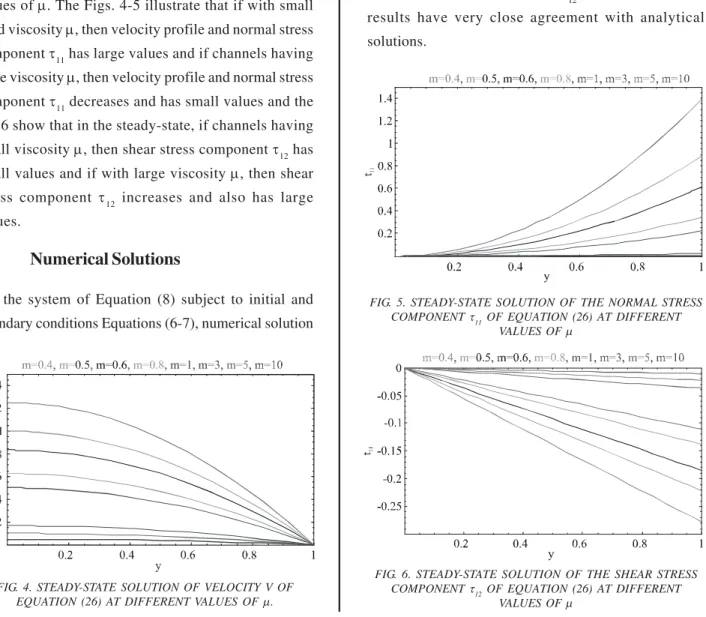
Steady-state solutions are plotted in Figs. 4-6 at different

values of μ. The Figs. 4-5 illustrate that if with small fluid viscosity μ, then velocity profile and normal stress component τ₁₁ has large values and if channels having large viscosity μ, then velocity profile and normal stress component τ₁₁ decreases and has small values and the Fig.6 show that in the steady-state, if channels having

small viscosity μ, then shear stress component τ₁₂ has small values and if with large viscosity μ, then shear stress component τ₁₂ increases and also has large values.

3.3

Numerical Solutions

For the system of Equation (8) subject to initial and

boundary conditions Equations (6-7), numerical solution

is resolute adopting function NDSolve of Mathematica

solver. Solutions are plotted in the Figs. 7-9, with increasing

time to compare against above analytical solution obtained

by Lie Group technique and displayed in Figs. 1-3. Fig. 7

illustrates that as time proceeds from rest, the velocity

profile of the flow increase in parabolic fashion and reached

at maximum value of v=0.5 from transition to steady-state.

Similarly, in Fig. 8 the normal stress component τ₁₁ has also similar trend of increase in non-linear style as time

increased from initial state and reached at a maximum value

of τ₁₁=0.22. Whilst, in Fig. 9 the shear stress component

τ₁₂ demonstrate linear tendency of increase in negative direction and attain at the value of τ₁₂=-0.11. The numerical results have very close agreement with analytical

solutions.

FIG. 4. STEADY-STATE SOLUTION OF VELOCITY V OF EQUATION (26) AT DIFFERENT VALUES OF μ.

FIG. 5. STEADY-STATE SOLUTION OF THE NORMAL STRESS COMPONENT τ₁₁ OF EQUATION (26) AT DIFFERENT

VALUES OF μ

FIG. 6. STEADY-STATE SOLUTION OF THE SHEAR STRESS COMPONENT τ12 OF EQUATION (26) AT DIFFERENT

4.

SOLUTION OF VISCOELASTIC

FLOW THROUGH CHANNEL

FILLED WITH POROUS MEDIA

The system of Equation (5) represents the flow of viscoelastic fluid in channels filled with porous media adopting Oldroyd-B constitutive model, solved as:

4.1.

Lie-point Symmetries

The problem of Equation (5) can be admitted into Lie group transformations if and only if:

0 ) 5 . 2 ( ) 12 12 1 ( ] 1 [

0 ) 5 . 2 ( ) 11 11 12 2 ( ] 1 [

0 ) 5 . 2 ( ) Re / 12 2

1 ( ] 2 [

= −

−

= −

−

= −

− + +

t We y

v X

t We y

v We X

t v Da v y yy v X

τ τ μ

τ τ τ

τ μ

(27)

Substituting the expansion of Equation (13) into the symmetry conditions of Equation (27). Then equating and separating them by the derivatives of v, τ₁₁, τ₁₂ and their powers lead to the over determined system of linear partial differential equations and after solving the system of linear PDEs, the result of the linear equating system gives rise the values of φ, ξ, η1_, η2 _and η3 _{in the following form:}

and

12 3 3 and

) ( 11 3 2 2

, Re 4 ) ( 3 1 , 2 , 1

τ η

τ η

η ξ φ

c

We t e y f c

Da t

e c Da v c c c

=

− + =

− + − = = =

(28)

where f(y) is an arbitrary function of y.

In Equation (28), ci are arbitrary constants and symmetry Lie algebra of system of partial differential of Equations (5) is four-dimensional and spanned by the following generators:

FIG. 7. NUMERICAL SOLUTION OF THE VELOCITY V OF THE SYSTEM OF EQUATION (8) SUBJECT TO INITIAL AND BOUNDARY CONDITIONS OF EQUATIONS (6-7) WITH Re=1,

μ₁=1/9, μ₂=8/9 AND We=1 AT DIFFERENT TIME t

FIG. 8. NUMERICAL SOLUTION OF THE NORMAL STRESS COMPONENT τ11 OF THE SYSTEM OF EQUATION (8)

SUBJECT TO INITIAL AND BOUNDARY CONDITIONS OF EQUATIONS (6-7) WITH Re=1, μ₁=1/9, μ₂=8/9 AND We=1 AT

DIFFERENT TIME t

FIG. 9. NUMERICAL SOLUTION OF THE NORMAL STRESS COMPONENT τ₁₂ OF THE SYSTEM OF EQUATION (8) SUBJECT TO INITIAL AND BOUNDARY CONDITIONS OF EQUATIONS (6-7) WITH Re=1,μ₁=1/9, μ₂=8/9 AND We=1 AT

Analytical Solutions of Viscoelastic Flow through Porous Channels 11 ) ( and Re 4 12 12 11 11 2 ) ( 3 , 2 , 1 τ τ τ τ τ ∂ ∂ − = ∝ ∂ ∂ − = ∂ ∂ + ∂ ∂ + ∂ ∂ − = ∂ ∂ = ∂ ∂ = We t e y f X v Da t e X v Da v X y X t X (29)

4.2

Solutions

Here only those operators are used that related to solution of physical problem of Equation (5) subject to initial and boundary conditions of Equations (6-7). Method of solutions depends on the applications of Lie group of transformation related with one-parameter to the system of partial differential of Equation (5).

4.2.1

Invariant Solution Corresponding to

X

₁

+

α

αα

α

α

X

₄

v Da t e t X X X ∂ ∂ − + ∂ ∂ = +

= ₁ α ₄ α Re

The invariant solutions under the operator X₁+αX₄ is given by:

⎪

⎪

⎭

⎪

⎪

⎬

⎫

= = − − = ) ( 3 ) , ( 12 ) ( 2 ) , ( 11 Re Re ) ( 1 ) , ( y y t y y t Da t e Da y y t v β τ β τ α β (30)

Substituting Equation (30) into the system of Equation (5) yields system of ODEs for β₁(y), β₂(y) and β₃(y).

⎪

⎪

⎭

⎪

⎪

⎬

⎫

= − ′ = − ′ = + − ′ + ′′ 0 ) ( 3 ) ( 1 1 0 ) ( 2 ) ( 1 ) ( 3 2 0 1 ) ( 1 1 ) ( 3 ) ( 1 2 y y y y y We y Da y y β β μ β β β β β β μ (31)

In Equation (31), prime stands for derivatives of y. It can be seen that this system of Equation (31) admit the following solutions: ⎪ ⎪ ⎪ ⎪ ⎭ ⎪⎪ ⎪ ⎪ ⎬ ⎫ + = + = + + = ) 2 1 ( 1 ) ( 3 2 ) 2 1 ( 1 2 ) ( 2 2 1 ) ( 1 Da y Cosh c Da y Sinh c Da y Da y Cosh c Da y Sinh c Da We y Da Da y Sinh c Da y Cosh c y μ μ μ μ β μ μ μ μ β μ μ β (32)

Substituting the values of Equation (32) into Equation

(30) and applying conditions of Equations (6-7), then the

system of Equation (5) admit the following solutions:

⎪ ⎪ ⎪ ⎪ ⎪ ⎪ ⎪ ⎪ ⎭ ⎪⎪ ⎪ ⎪ ⎪ ⎪ ⎪ ⎪ ⎬ ⎫ − − − = − − = − − − = Da Cosh Da y Sinh Da t e Da y t Da Cosh Da y Sinh Da t e Da We y t Da Cosh Da y Cosh Da t e Da y t v μ μ μ μ τ μ μ μ μ τ μ μ 1 ) Re 1 ( 1 ) , ( 12 1 2 2 2 ) Re 1 ( 1 2 ) , ( 11 ) 1 1 ( ) Re 1 ( ) , ( (33)

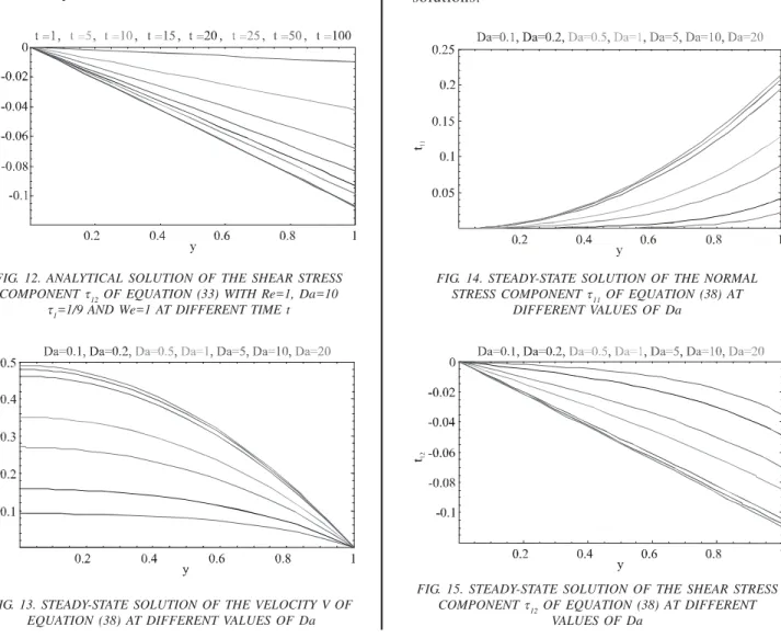
These solutions of Equation (33) are expressed in Figs.

10-12 for several of parameters at different time t.

The time dependent effect on the axial velocity, normal

stress component and shear stress are displayed in Figs.

velocity increases as the time increases and there is an

upper limit for this increase, as time t>60 velocity reaches

at steady-state. Similarly effect of normal stress

componen τ₁₁ and shear stress component τ₁₂ are shown in Figs. 11-12. These figures depict that normal stress

component τ₁₁ increases at an increased for values of time and there is also an upper limit for this increase,

There is no further change in normal stress as time

reaches beyond the value of t=60 units, and the shear

stress component τ₁₂ decreases as time increases and there is a lower limit for this decrease. Shear stress tends

to steady-state after time t>60.

4.2.2

Invariant Solution Corresponding to X

₁

The invariant solution associated with X₁ is the steady-state solution:

(34)

Substituting Equation (34) into system of Equation (5) yields system of ODEs for ϕ(y), ψ(y), and φ(y):

(35)

Subject to boundary conditions:

ϕ(-1) = 0 and ϕ(1) = 0 (36)

After integration of Equation (35), the result is given as:

(37)

Applying the boundary conditions of Equation (36), system of partial differential of Equations (5) admit the steady-state solutions as under"

(38)

FIG. 10. ANALYTICAL SOLUTION OF THE VELOCITY V OF EQUATION (33) WITH Re=1, Da=10 AT DIFFERENT TIME t

FIG. 11. ANALYTICAL SOLUTION OF THE NORMAL STRESS COMPONENT τ11 OF EQUATION (33) WITH Re=1, Da=10

Analytical Solutions of Viscoelastic Flow through Porous Channels

Steady-state solutions are plotted in Figs. 13-15 at different values of Da.

The steady-state velocity, normal stress component and

shear stress are displayed in Figs. 13-15 respectively.

The Figs. 13-14 shows that in the steady-state, if

channels having small Da, then steady velocity v and

steady normal stress component τ₁₁ have small values that if permeability decreases, then resistance increases

and hence velocity decreases and normal stress τ₁₁ also decreases in the steady-state, and Fig .15 shows that in

the steady-state, if channels having small Da, steady

shear stress component τ₁₂ have large values that is if permeability decreases, then shear stress τ₁₂ increases in the steady state.

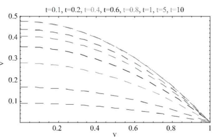
4.3

Numerical Solution

Numerical solution are obtained for the system of PDEs of Equation (5) subject to initial and boundary conditions of Equations (6-7) using NDSolve in Mathematica solver and are plotted in the Figs. 16-18 with increasing time. Fig. 16 shows that as time proceeds, the channel velocity increases and reaches at steady-state as time approaches beyond six units (t>6). Similarly, in Fig. 17 the normal stress component

τ₁₁ illustrate increases with respect to time and achieve steady-state at same time level with similar non-linear fashion. Whilst, in Fig. 18 the behaviour of shear stress is illustrated which clearly indicate the linear trend. All numerical results are comparable with analytical solutions.

FIG. 12. ANALYTICAL SOLUTION OF THE SHEAR STRESS COMPONENT τ12 OF EQUATION (33) WITH Re=1, Da=10

τ1=1/9 AND We=1 AT DIFFERENT TIME t

FIG. 13. STEADY-STATE SOLUTION OF THE VELOCITY V OF EQUATION (38) AT DIFFERENT VALUES OF Da

FIG. 14. STEADY-STATE SOLUTION OF THE NORMAL STRESS COMPONENT τ11 OF EQUATION (38) AT

DIFFERENT VALUES OF Da

FIG. 15. STEADY-STATE SOLUTION OF THE SHEAR STRESS COMPONENT τ₁₂ OF EQUATION (38) AT DIFFERENT

FIG. 16. NUMERICAL SOLUTION OF THE VELOCITY V OF SYSTEM OF EQUATIONS (5-7) WITH Da=10, Re=1, μ1=1/9,

μ₂=8/9 AND We=1 AT DIFFERENT TIME t

FIG. 17. NUMERICAL SOLUTION OF THE NORMAL STRESS COMPONENT τ₁₁ OF THE SYSTEM OF EQUATIONS (5-7)

WITH Da=10, Re=1, μ1=1/9, μ2=8/9 AND We=1 AT

DIFFERENT TIME t

FIG. 18. NUMERICAL SOLUTION OF THE SHEAR STRESS COMPONENT τ12 OF THE SYSTEM OF EQUATIONS (5-7)

WITH Da=10, Re=1, μ₁=1/9, μ₂=8/9 AND We=1 AT DIFFERENT TIME t

5.

CONCLUSIONS

Analytical solutions are obtained successfully by

employing Lie group technique for both velocity profile

and non-linear Oldroyd-B stress constitutive equation

coupled with momentum equation. From the results, it

is observed that velocity and first normal stress

components have increasing trends against increasing

time and turns to be steady state at non-dimensional

time greater than 50 and smaller than 75 units

respectively. Whereas shear stress component

decreases as time increases and becomes steady state

at time greater than 75.

Whilst, in the steady state, velocity profiles and first

normal stress components, at different values of

viscosity and Darcy's number are observed with

increasing trend against increasing values of viscosity

and Darcy's number. Whereas, shear stress component

is observed decreasing trend as viscosity or Da

increases. Comparison has been made against analytical

and numerical solutions and is found very close

agreement to one another.

ACKNOWLEDGEMENTS

Financial support of HEC and Department of Mathematics,

Shah Abdul Latif University, Khairpur, Mirs, Pakistan, is greatly acknowledged.

REFERENCES

[1] Arada, N., and Sequeira, A., “Strong Steady Solutions for a Generalized Oldroyd-B Model with Shear Dependent Viscosity in a Bounded Domain”, Mathematical Models in Applied Sciences, World Scientific Publishing Company, Volume 13, No. 9, 2003.

Analytical Solutions of Viscoelastic Flow through Porous Channels [3] Park, K.S., and Known, Y.D., “Numerical Description

of Start-Up Viscoelastic Plane Poiseuille Flow”, Korea-Australia Rheology Journal, Volume 21, No. 1, pp. 47-58, March, 2009.

[4] Larson, R.G., “Constitutive Equations for Polymer Melts and Solutions”, Butterworth Publishers, 1988. [5] Larson, R.G., “The Structure and Rheology of Complex

Fluids”, Oxford University Press, 1999.

[6] Tan, W.C., and Masuoka, T., 'Stokes' First Problem for a Second Grade Fluid in a Porous Half-Space with Heated Boundary”, International Journal of Non-Linear Mechanics, Volume 40, No. 4, pp. 515-522, 2005. [7] Tan, W.C., and Masuoka, T., “Stokes' First Problem for

an Oldroyd-B Fluid in a Porous Half Space”, Physics of Fluids, Volume 17, No. 2, Article ID 023101, pp. 7, 2005.

[8] Tan, W.C., and Masuoka, T., “Stability Analysis of a Maxwell Fluid in a Porous Medium Heated from Below”, Physics Letters A, Volume 360, No. 3, pp. 454-460, 2007.

[9] Tan, W.C., “Velocity Overshoot of Start-Up Flow for a Maxwell Fluid in a Porous Half Space”, Chinese Physics, Volume 15, No. 11, pp. 2644-2650, 2006.

[10] Carew, E.O., Townsend, P., and Webster, M.F., “A Taylor-Petrov-Galerkin Algorithm for Viscoelastic Flow”, Journal of Non-Newtonian Fluid Mechanics, No. 50, pp. 253-287, 1993.

[11] Baloch, A., “Numerical Simulation of Complex Flows of Non-Newtonian Fluid”, Ph.D. Thesis, University of Wales Swansea. November, 1994.

[12] Birkhoff, G., “Mathematics of Engineers”, Electrical Engineering, No. 67, pp. 1185-1192, 1948.

[13] Morgan, A.J.A., 'The Reduction by one of the Number of Independent Variables in Some Systems of Nonlinear Partial Differential Equations”, Quarterly Journal of Mathematics, No. 3, pp. 250-259, 1952.

[14] Basov, S., “Hamiltonian Approach to Multi-Dimensional Screening”, Journal of Mathematics Economics, No. 36, pp. 77-94, 2001.

[15] Basov, S., “A Partial Characterization of the Solution of the Multidimensional Screening Problem with Nonlinear”, Department of Economics, the University of Melbourne, Research Paper No. 860, 2002.

[16] Basov, S., “Lie Groups of Partial Differential Equations and Their Application to the Multidimensional Screening Problems”, Department of Economics, The University of Melbourne, 2004.

[17] Fayez, H.M., and Abd-el-Mmalek, M.B., “Symmetry Reduction to Higher Order Nonlinear Diffusion Equation”, International Journal of Applied Mathematics, No. 1, pp. 537-548, 1999.

[18] Moran, M.J., and Gaggioli, R.A., 'Reduction of the Number of Variables in System of Partial Differential Equations with Auxiliary Conditions”, Journal of Applied Mathematics, pp. 202-215, 1968.

[19] Bluman, G.W., and Kumei, S., “Handbook of Symmetries and Differential Equations”, New York, Springer, 1989.

[20] Olver, P.J., “Handbook of Applications of Lie Groups to Differential Equations”, New York, Springer, 1986.

[21] Ibragimov, N.H., “Handbook of Elementary Lie Groups Analysis and Ordinary Differential Equation”, New York, Wiley, 1999.

[23] Jena, J., "An Algorithm for Solutions of Linear PartialDifferential Equations via Lie Group of Transformations", Applied Mathematical Sciences, Volume 5, No. 27, pp. 1337-1347, 2011.

[24] Jalil, M., Asghar, S., and Mushtaq, M., "Lie Group Analysis of Mixed ConvectionFlow with Mass Transfer Over a Stretching Surfacewith Suction or Injection", Mathematical Problems in Engineering, Hindawi Publishing Corporation, pp. 14, 2010.

[25] Sahin, D., Antar, N. and Ozer, T., "Liegroup Analysis of Gravity Currents", Nonlinear Analysis: Real World Applications, No. 11, pp. 978-994, 2010.