*e-mail: [email protected]
The Effect of Adding Boron in Solidification Microstructure of Dilute
Iron-Carbon Alloy as Assessed by Phase-Field Modeling
Henrique Silva Furtadoa*, Américo Tristão Bernardesb,
Romuel Figueiredo Machadob, Carlos Antônio Silvab
a
ArcelorMittal Tubarão, Av. Brigadeiro Eduardo Gomes, 930, Serra, ES, Brasil
bDepartamento de Física, Rede Temática em Engenharia de Materiais – REDEMAT,
Universidade Federal de Ouro Preto – UFOP, Campus Morro do Cruzeiro,
Ouro Preto, MG, Brasil
Received: November 10, 2010; Revised: March 21, 2011
Alloying element like boron, even in small addition, is well known to improve hardenability of steels. Its application can improve mechanical properties of steels and reduce alloying costs. Despite these benefits is not easy to cast boron steels, mainly in dynamical solidification process like continuous casting, due to their crack susceptibility1,2. The strategy of using Phase-Field simulation of the solidification process is based on its proved
capacity of predicting realistic microstructure that emerge during solidification under conditions even far from equilibrium3-5. Base on this, some comparative simulations were performed using a three component dilute
alloy in a two dimensional domain under unconstrained (isothermal) and constrained (directional) solidification. Simulation results suggested two fragile mechanisms: one related to a deep dendritic primary arms space and other due to the remelting of this region at low temperature. Both resulted mainly from the high boron segregation in interdendritic regions.
Keywords: Phase-Field, solidification, dilute alloys, boron, Fe-C alloys
1. Introduction
Phase-Field model is an approach based on the concept introduced by Gibbs and Van der Waals, which states that solid-liquid interface has a physical dimension of nanometer magnitude3,6,7. It is widely
accepted for prediction of solidification microstructure of pure substance as well as alloys of different solute contents3-5. For two
phases system it uses an order parameter (φ) as a state variable that identify the phases, i.e., it is constant inside the bulk phase (ex: 0 for liquid and 1 for solid) and change continuously between these values along the interface3. It does not have the disadvantage of tracking
the interface all the time. In fact the model solution determines its position.
Developments of Phase-Field models can be addressed to Van der Waals who perceived that the addition of gradient term in free energy functional has an effect of creating interface with certain thickness6.
Cahn and Hilliard8, after rediscovering this idea, associated it to
the interfacial tension and solid-liquid interface thickness, allowing Phase-Field model parameters to be related to them.
Important contribution came from Langer6 who proposed the
first Phase-Field model for solidification of pure substances. No less important was the pioneer work from Kobayachi9, whose first
numerical simulation introduced the formalism to incorporate anisotropy that is used until present date.
In general, Phase-Field models of solidification of three component alloys without convection in liquid or solid state tension effects are composed by four diffusion equations: one for the order parameter; one for temperature and two for the solutes. These can be phenomenological, based on free energy functional or developed from entropy functional3,7. Despite both approaches reproduce similar
results3, the most used one is the phenomenological, mainly due to
its faster convergence and its facility to obtain model parameters based on material properties3. Therefore, according to Cahn and
Hilliard8 and Landau Ginsburg7 the free energy functional (F) can
be formulated as follows:
(
)
2 2, , 2
i
F=∫f φN T +ξ ∇φ dV
(1)
where f (φ, Ni, T) is a free energy density that is function of order parameter (φ), concentrations of solutes (Ni) and temperature (T); ξ
is a energy density contribution from the gradient of order parameter and V is system’s volume.
The key point of the phenomenological Phase-Field model is to consider that free energy decreases monotonically as solidification advances, i.e:
. F
M t
∂φ= − δ
∂ δφ (2)
where t is time and M is a Phase-Field mobility term. From the derivative of this functional it follows the general expression for the diffusion of order parameter:
2 2
. f
M t
∂φ ∂
= − − ξ ∇ φ
∂ ∂φ (3)
In order to describe f (φ, Ni, T) it has been used a weighing rule3,
defined as followed:
(
)
( )
( )
(
)
( )
(
)
(
)
.
, , ,
.
1 ,
s
i p i
L i
f N T W h f N T
hp f N T
φ = Φ φ + φ
+ − φ
(4)
where hp (φ) is an interpolation function which varies along solid-liquid interface from a fixed value in solid (ex.: hp (1) = 1) to a fixed value in liquid (ex.: hp (0) = 0), W is the interface energy density and
Φ(φ) is a double well function. In the above expression (Equation 4) the first term of right side is related to the interface energy and the others are the bulk free energy of solid (fS) and liquid (fL) phases,
respectively.
and isotropic material without noise in an one dimension domain, it is possible to relate these parameters to the interfacial tension (σ) and interface thickness (2λ) as follows11:
0
. 3 2
.
W
ξ = σ (14)
0
. 2.94 2.
. 2
W = ξ
λ (15)
The Phase-Field mobility term (M0) formulation was developed for alloys by Karma12 using asymptotic analysis and independently
by Kim et al.13 using solidification kinetic consideration.
Echebarria et al.14, based on work of Karma12, developed a model
for 2 components alloy without diffusion in solid (one side model). Ode et al.15 proposed another approach for a three component alloy,
however, considering the same simplification and vanishing inverse of kinetic coefficient (β). On the other side, Ramires et al.16 presented
an alternative formulation for 2 components alloy, considering a non-isothermal domain, no diffusion in solid and vanishing inverse of kinetic coefficient. More recently, Kim10 reviewed this development
and proposed a new formulation for multicomponent alloy, however, considering the same simplifications of Ode et al.15. In this context, a
recent work by Ohno et al.17 for a 2 component alloys was developed
to deal with diffusion in solid. They17 considered an isothermal case
and vanishing inverse of kinetic coefficient, obtaining results17 similar
to the one side model.
Based on Kim10, Ramires at al16 and Ohno et al.17 the present work
employs a custom developed approach to three component alloy, for non-isothermal conditions, non-vanishing kinetic coefficient and diffusion in solid described by the following expression:
(
)
(
)
2 2 1 1 2 1 0 0 2 2 2 2 2. . 1 .
. . .
1
.
. 2. . . .
1 . .
Le
f M
L
T m f
f Le m M L m f
H R T k N
K D V H
H A
M T W R T k N
D V H
∆ −
+
∆
ξ ∆ ξ
= β +
σ −
+
∆
(16)
where DL
i (i = 1, 2) are liquid solute diffusivities and Ni Le are
equilibrium solute concentrations in liquid phase, which can be obtained from phase diagrams, KT is the thermal conductivity and A is a constant. This formulation reduces to the one from Ramires et al.16
for two components alloy as well as to the one from Karma Rappel18
for pure materials.
The solute diffusion equations are based on conservative Onsager extrapolation without cross effect on diffusivities terms (Di,l), i.e.:
. 1 n i i l l l N f D
t = N
∂ ∂
= ∇ ∑
∂ ∂ (17)
Using Kim10 approach and the ‘antitrapping’ correction term
from Karma12
( )
i
j
the expression for non-dimensional solute concentrations (Ui) can be written as follows:
( )
( )
.(
. 1(
)
1)
L i
i i i i d i i
U
D q U j h U k
t t
∂ ∂
= ∇ φ ∇ + + φ − +
∂ ∂
(18)
where
( )
d( )
. iS(
1 d( )
)
. iLi L
i
h D h D
q
D
φ + − φ
φ = (19)
and Hence, it is possible to obtain a general formulation for the order parameter diffusion equation, i.e.:
(
2 2)
M source W t
∂φ
= − + Φ′− ξ ∇ φ
∂ (5)
where Φ´ is the derivative of Φ in relation to φ and source depends on the bulk free energy of solid and liquid phases.
Following the multicomponent approach from Kim10 and
considering constants solutes activity coefficients of infinite dilution, it is possible to obtain the following expression (see detailed development in Appendix A):
( )
(
)
(
)
(
(
)
)
2 1 . .. . . 1
. . 1 1
m f m p i i i i i m T T H T source h
R T N k
U k V ∞ = − ∆ +
= − ′ φ
− ∑ − + (6) where
( )
/(
( )
)
1 .1 . 1
i i
i
i i r r
N N
U
k k h h
∞
=
− φ + − φ (7)
where Tm is the melting temperature of pure solvent, R is the universal gas constant, ∆Hf is the enthalpy of fusion of pure solvent, Vm is the alloy molar volume, ki are the solutes equilibrium solute partition coefficients, Ni∞ are the initial alloy solute concentrations and hr(φ) is another interpolation function with the same properties of hP(φ).
In order to simulate complex microstructure, anisotropy was included in the model as proposed by Kobayachi9, where the
parameters ξ and M were made to vary according the angle (θ) between solid-liquid interface normal vector and horizontal axis (x) in the present domain of two dimensions (2D). The final diffusion Equation for the order parameter is as follows:
( )
( )
( ) ( )
( ) ( )
2 1 . .M t y x
W source noise
x y
∂φ= ∇ξ θ ∇φ + ∂ξ θ ξ θ′ ∂φ
θ ∂ ∂ ∂
∂ ∂φ
− ξ θ ξ θ′ − Φ +′ +
∂ ∂
(8)
In this case the following expressions were used7:
/ tan / y Arc x
∂φ ∂
θ =
∂φ ∂
(9)
( )
0. 1{
ξ.cosj(
0)
}
ξ θ = ξ + δ θ − θ (10)
( )
∂ξ θ( )
ξ θ =′∂θ (11)
( )
0.{
1 M.cos(
0)
}
M θ =M + δ jθ − θ (12)
(
)
2. . . .
16 1
noise= Aν φ − φ (13)
where δξ and δM are the strength of anisotropy, j is the number of anisotropy, θ0 is the main growth angle, A is the amplitude of noise and ν is random number obtained from a uniform distribution.
Predictions for ξ0 and W follows from the work of Cahn and Hilliard8 on surface tension. In that case and considering the analytical
avoids joint thermodynamic and Phase-Field calculations inside each time step, reducing the numerical processing time.
Isothermal solidification constitutes the maximum rate of solidification of unconstrained dendrite growth. The alloys were submitted to different undercoolings and their solid-liquid interface evolutions were determined until reaching steady state condition. The interface thickness (2λ) was set up to 8 × 10⁻⁸ m and the inverse of
kinetic coefficient was estimated as an arithmetic average between pure iron, determined by collision limited teory22, and the value
reported by Ogushi e Suzuki23 for a higher carbon Fe-C alloy, i.e.:
0.54 s.m/K. The properties used in simulation are summarized in Table 1. The results presented in Figure 3 show that boron addition has the effect of narrowing the dendrite primary arm thickness. That phenomenon can be attributed to the tip radius selection, associated to the boron solute gradient around the solid-liquid interface.
In order to determine the dendrite tip radius, a parabolic function (fy) was fitted to data close to the main dendrite tip arm. This is a plausible approach which is based on experimental evidences24.
Thus tip radii (r) formed in different solidification velocity were determined using the following formulas:
1
r K
= − (22)
where
(
2)
3/2''
1 '
fy K
fy
=
+ (23)
Here fy´ and fy´´ are the first and the second order spatial derivative of fy in relation to x direction (horizontal direction) and
K is the curvature of the dendrite main tip arm. The results of this analysis are summarized in Figure 4. It shows that the dendrite tip radius decrease as solidification velocity increases until a limit where it starts to increase. This point is related to the high velocity dendrite-cellular morphological transition24. It is a common behavior of all
three alloys. In these cases, the increase of boron addition reduced the dendrite tip radius and also it seems to reduce the velocity where this transition should happen.
According to the marginal stability theory, the tip selection is a result of stabilizing forces (e.g.: solute gradients) and non-stabilizing forces (interfacial tension), modulated by the selection parameter24, which is commonly used in one dimensional analytical
tip model as a easier tool to map the morphological transition of materials under solidification. However is not easy to determine this parameter because it can depend on alloy composition and anisotropy. Nonetheless, Phase-Field simulation can be used to estimate it, and for the three alloys under consideration the results are summarized in Table 3. It seems that the higher the boron content the higher the selection parameter.
(
)
. .1 1 . 2
i i i
j k U
t W
ξ ∂φ ∇φ
= + − ∂ ∇φ
(20)
where DS
i are solid solute diffusivities and hd(φ) is another interpolation
function with the same properties of hP(φ) and hr(φ).
In order to describe the temperature field in directional solidification, a quasi-steady state approximation was used14. It takes
in consideration a sample traveling in one direction (ex. z) with a constant pulling velocity (ex. VP) under a fixed thermal gradient (G). This approach can be implemented as follows:
(
)
0 . p.
T=T +G z−V t (21)
where T0 is the initial temperature.
Equations 8 and 18 were solved using finite volume method19
with uniform grid. For the time derivative, the explicit scheme was used. Despite some limitation regarding the definition of the time step, it is easy to implement and has the advantage that the Phase-Field Equation does not need to be solved outside the interface region.
2. Results and Discussion
This model was already validated against analytical solution and experimental data for pure material and 2 components alloys20,21.
However, some new calculations were first performed in order to compare their results with equilibrium thermodynamic data for dilute ternary alloys. As far as the rate of solidification is small, solute concentration should approach the values given byphase diagrams. That constitutes an additional validation procedure.
The first analysis was performed for Fe (BCC)-C-P dilute alloy. Input data are summarized in Table 1. Phase-Field model was set up to use a flat interface thickness (2λ) of 8,0 × 10⁻⁸ m and vanishing
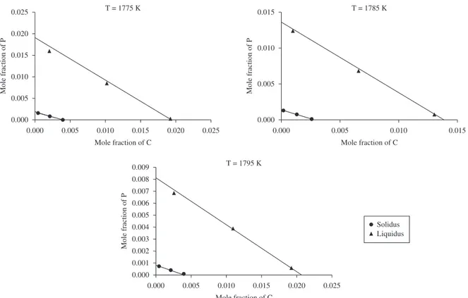
inverse kinetic coefficient. The domain was defined with 3 nodes in horizontal direction. Anisotropy effect and noise were set up to zero. A flat solid-liquid interface was allowed to advance in vertical direction until reaching steady state. The resulting solute concentration profiles of carbon and phosphorus are presented in Figure 1 together with three isothermal slices of dilute Fe(BCC)-C-P phase diagram reported by Ode et al.15. The agreement is remarkable.
A second Phase-Field calculation was focused on Fe(BCC)-C-B dilute alloy. The procedure was similar to that applied to the Fe(BCC)-C-P dilute alloy. Again, input data are from Table 1. As it can be seen from Figure 2, a good agreement was obtained between the present Phase-Field calculations and phase diagram data obtained from Blasek et al.1.
In order to analyze the effect of boron on the solidification microstructure, the present work simulated three alloys with different boron contents (Table 2). Their equilibrium solute concentrations necessary to determine the mobility parameter M (Equation 16) were determined previously as function of temperature. This procedure
Table 1. Data used in the present Phase-Field calculation.
Properties Fe-C15 Fe-P15 Fe-B1
Melting temperature of pure iron (K) 1811 1811 1811
Equilibrium solute partition coefficient 0.204 0.102 0.053
Liquidus slope (K.mole–1) –1802 –1836 –1964
Interfacial tension (J.m–2) 0.204 0.204 0.204
Solute diffusivity in liquid phase (m2/s) 2.0 × 10⁻⁸ 1.7 × 10⁻⁹ 1.0 × 10⁻⁸
Solute diffusivity in solid phase (m2/s) 6.0 × 10⁻⁹ 5.5 × 10⁻¹¹ 2.05 × 10⁻¹⁰
Figure 1. Solid-liquid equilibrium solute concentration in dilute Fe(BCC)-C-P alloy: points determined by the present Phase-Field model; lines are from equilibrium phase-diagram.
The addition of boron in the dilute Fe(BCC)-C alloy should increase the non-stabilizing forces during solidification because it creates an extra solute diffusion field. Therefore one should expect an increase of solid-liquid interface disturbances at a certain solidification velocity. In order to verify this effect, the domain and the simulation time were expanded. The way to perform this is to increase the solid-liquid interface thickness. It has been shown that is possible to obtain convergence of Phase-Field simulation to the analytical solution of Mullins Sekerka instability theory, and therefore to obtain consistent results, using interface thickness smaller than dendrite tip radius14. In order to make this simulation feasible with
the present model, the interface thickness (2λ) was increased to 2 × 10⁻⁷ m. The grid size and the time step were set up to 5.0 × 10⁻⁸ m
and 5.0 × 10⁻⁹ s, respectively. Morphological results on the three alloys
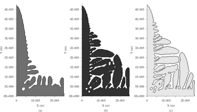
under analysis can be compared in Figure 5. Actually, it seems that, for similar solidification time, the increase of boron addition lead to an intensification of secondary arms growth. Also, it can be observed some indication of secondary arms dynamic coalescence phenomena, where larger arms grow faster and smaller ones are melted back. This suggests that boron addition can lead to an increase in the secondary arms spaces due to increasing dynamic coalescence, which is in agreement with the theory of secondary arms growth22.
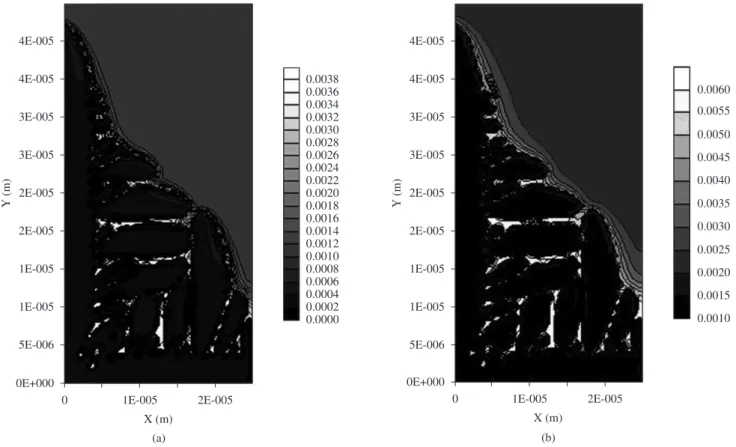
Solute segregation is an important phenomenon that can strongly influence macroscopic properties of materials. Regarding this, Figure 6 and 7 show the carbon and boron segregation resulting from morphologies presented before (Figure 5). It is clear the increase of carbon and boron concentrationsin the interdendritic regions. These higher concentrations could lead, according to Blasek et al.1, to a
low temperature remelting (around 1200 °C) of already solidified interdendritic region. This phenomenon has been associated to the ductility loss and crack formation during continuous casting of boron steel1.
In directional solidification (constrained growth) the solidification front is inside the range defined by solidus and liquidus temperature. At steady state, pulling velocity is equal to the solidification velocity and morphology is mainly columnar, which is the most common microstructure in continuous casting process. In order to simulate this process, Equation 21 was included in the present Phase-Field model. However, typical continuous casting cooling rate is not feasible to be simulated with the present implementation due to the large domain and time required to resolve the microstructure, which would result in a huge processing time (ex.: a system with 108 grid points and
107 time steps). Therefore a faster cooling rate was set up based on
work of Miettinen25. In this case, fixed values of temperature gradient
(G), pulling velocity (Vp) and initial temperature (T0) were set up. Two seeds were implemented in both upper and lower left corner of the domain. The distance between them was defined by primary arms space asdetermined by Miettinen25 for these conditions, i.e.:
1.5 × 10⁻⁵ m. The dimension of the domain in the other direction (now
z direction) was set up in order to have a well developed microstructure and, at same time, ensure a certain superheat at the high side of the domain, i.e.: 7.5 × 10⁻⁵m. Interface thickness, grid size and time step
were defined as 3 × 10⁻⁷ m, 7.5 × 10⁻⁸ m, 2 × 10⁻⁸ s, respectively.
Table 2. Iron–carbon alloys simulated in present work.
Alloy C (mole fraction) B(mole fraction)
FeC 0.00232 0.000000
FeCB1 0.00232 0.000515
FeCB2 0.00232 0.001030
Table 3. Selection parameter for the 3 alloys simulated by the present Phase-Field model.
Alloy Range of solidification velocity (m/s)
Selection parameter FeC 0.054 to 0.298 0.0446 FeCB1 0.016 to 0.020 0.0598 FeCB2 0.027 to 0.204 0.0762
Figure 4. Effect of boron addition on tip radius-solidification velocity relation.
Figure 5. The effect of boron addition on dendrite secondary arms growth: a) alloy FeC; b) alloy FeCB1; and c) alloy FeCB2.
Field simulations. Therefore, in order to reduce the susceptibility for crack formation in this steel one should focus on minimizing boron segregation. As product hardenability improvement is due to the presence of solid soluble boron1 and, as reported before, its
solubility in this phase is very low (figures 8 and 9), the first approach should be the reduction of its addition to a minimum defined by its solubility limit in solid phase. Another possible strategy would be the use of another element capable of forming a high temperature third phase with boron.
It is important to point out that present simulation were performed using properties independent of temperature and concentrations. Nonetheless, the excellent agreement of Phase Field results with equilibrium phase diagrams indicates that this simplification can work properly concerning dilute solution.
Another point is on some larger values used in present work to define interface thickness necessary to extend the simulation domains. In this regard, the present Phase-Field model were implemented using the ‘antitraping’ flux (Equation 20), therefore one can not expect any artificial solute trapping, which could reduce solute segregation close do solid-liquid interface. Besides, these values were always kept lower enough to resolve dendritic arms.
In actual continuous casting process the solidification front is expected to be sensitive to the liquid convection that can affect solute segregation. This phenomenon can be driven by fluid flow of liquid steel entering in the mould in the first stage of solidification and also by shrinkage of solid. Also, change in liquid density and surface tension gradient (Maragoni’s convection) can provoke convection, both due to concentration gradient formed at solidification front. As these phenomena were not include in the present Phase-Field model one should expect some differences between present results and actual process. Nonetheless, based on sample presented in Figure 10, The solid-liquid interface growth in directional solidification
is driven by constitutional undercooling, which in turn is defined by solute segregation at the interface. Simulation results on solute segregation using the present Phase-Field model can be seen in Figure 8, where the darkest areas correspond to the solid phase and the solute gradients between the two arms comes from segregation phenomena, where solid phase rejects solute to the liquid phase. From these results it is possible to determine the constitutional undercoolings, which are presented in Figure 9 (negative values). As it can be seen, the interdendritic region is not totally undercooled in the present simulation. Additionally it is noticeable that boron addition increases the interdendritic region making the main dendrite arms thinner. On the other side, close to dendrite tip, the constitutional undercoolings become higher as boron addition increases.
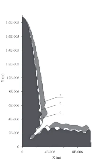
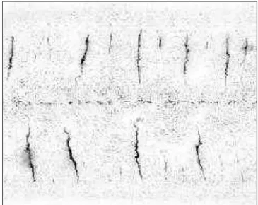
As a consequence of the above results, liquid fraction between the thinner arms increases, resulting in more fragile microstructure, which would be under transverse tensile stress common in continuous casting. Indeed, it has been reported severe crack formation parallel to the dendrite main axis during casting of high boron content steel, as shown in Figure 10, which is consistent with present Phase-Field simulations.
Based on simulation of present work, it can be concluded that two mechanisms making high boron alloyed steel to be more sensitive to crack formation during continuous casting could be present: one occurring at solidification front and other at lower temperature (around 1200 °C). The fist one could be related to a deep dendritic primary arms space that would concentrate the tensile stress common to the continuous casting process. The second one could be due to the remelting of this region at low temperature resulting in a large localized ductility loss. Both mechanisms resulted mainly from the high boron segregation in interdendritic regions, predicted by
Figure 8. Segregation fields of carbon and boron (mole): a) alloy FeC; b) alloy FeCB1; and c) alloy FeCB2.
Figure 9. Constitutional undercoolings determined from solute concentration profiles: a) alloy FeC; b) alloy FeCB1; and c) alloy FeCB2.
Figure 10. Sulfur print of a transversal slice of continuously casted slab of high boron steel2.
4. Provatas N and Greenwood M. Multiscale Modeling of Solidification: phase-field method to adaptive mesh refinement. International Journal of Modern Physics B. 2006; 19(31):4525-4565.
5. Steinbach I. Phase-Field Models in Materials Science: modelling and simulation in materials. Science and Engineering. 2009; 17(073001):1-30. 6. Langer JS. Models of Patherm Formation in First Order Phase Transition.
Direction in Condensed Matter Physics, World Science on Direction in Condensed Matter Physics, World Scientific Publishing. 1983; 1:165-168. 7. Emmerich H. The Diffusive Interface Approach in Materials Science: thermodynamic concepts and applications of phase-field models. Berlin Heidelberg: Springer-Verlag, 2003. doi:10.1007/3-540-36409-9
8. Cahn JW and Hilliard JE. Free Energy of a Nonuniform System: i- interfacial free energy. The Journal of Chemical Physics. 1958; 28(2):258-267. doi:10.1063/1.1744102
9. Kobayashi R. Modeling and Numerical Simulations of Dendritic Crystal Growth. Physica D. 1993; 63:410-423. doi:10.1016/0167-2789(93)90120-P
10. Kim SG. A phase-field model with antitrapping current for multicomponent alloy with arbitrary thermodynamic properties. Acta Materialia. 2007; 55:4391-4399. doi:10.1016/j.actamat.2007.04.004
11. Furtado AF. Modelamento do processo de Solidificacao de Microestruturas pelo metodo do campo de fase [tese]. Rio de Janeiro: Universidade Federal Fluminense; 2005.
12. Karma A. Phase-Field Formulation for quantitative Modeling of Alloy Solidification. Physical Review Letters. 2001; 83(11):115701-2-115701-4. 13. Kim SG, Kim WT and Suzuki T. Phase-Field model for binary
alloy. Physical Review E. 1999; 60(6):7186-7197. doi:10.1103/ PhysRevE.60.7186
14. Echebarria B, Folch R, Karma A and Plapp M. Quantitative Phase Field Modeling of Alloy Solidification. Physical Review E. 2004; 70(6):601-604.
15. Ode M, Lee JS, Kim SG, Kim WT and Suzuki T. Phase-Field Model for Solidification of Ternary Alloy. ISIJ international. 2000; 40(9):870-876. 16. Ramires JC, Beckermann C, Karma A and Dieper H-J. Phase-Field
Modeling of binary alloy solidification with coupled heat and solute diffusion. Physical Review E. 2004; 69(15):051607-1-051607-16. 17. Ohno M and Matsuura K. Quantitative Phase-Field Modeling for dilute
Alloy Solidification involving diffusion in the Solid. Physical Review E. 2009; 79:031603-1-031603-15.
18. Karma A and Rappel WJ. Quantitative Phase-Field Modeling of dendrite Growth in two and three Dimensions. Physical Review E. 1998; 57(4):4323-4349. doi:10.1103/PhysRevE.57.4323
19. Patankar SV. Numerical Heat transfer and fluid flow. New York: Hemisphere Publishing Corporantion; 1980. 197 p.
20. Furtado HS, Bernardes AT, Romuel RF and Silva CA. Two Dimensional Numerical Analysis of nickel and iron Dendritic Morphologies Using Phase-Field Method. Revista da Escola de Minas-REM. 2009; 62(2):199-204.
21. Furtado HS, Bernardes AT, Romuel RF and Silva CA. Numerical Simulation of Solute Trapping Phenomena Using Phase-Field Solidification Model for Dilute Binary Alloys. Materials Research. 2009; 12(3):345-351.
22. Stefanescus DM. Science and Engeneering of Casting Solidification. Kluwer, New York: Academic/Plenym Publisher; 2002. doi:10.1590/ S1516-14392009000300016
23. Oguchi K and Suzuki T. Free Dendrite Growth of Fe-0.5 mass%C Alloy- Three dimensional Phase-Field Simulation and LKT model. ISIJ International. 2007; 47(10):1432-1435. doi:10.2355/ isijinternational.47.1432
24. Trivedi R and Kurz W. Dendritic growth. International Materials Reviews.
1994; 39(2):25-49.
25. Miettinen F. Thermodynamic-Kinetic Simulation of Constrained Dendrite Growth in Steel. Metallurgical and Materials Transaction B. 2000; 31B:365-379. doi:10.1007/s11663-000-0055-6
convection. Therefore the final results could be a thinner dendritic primary arm thanthat predicted by the present work and, therefore, a deepest interdendritic region. i.e., the presence of convection could induce an increase in the fragility of solid-liquid front. However, in order to confirm the above comments it is important toinclude in the Phase-Field model the convection phenomenon.
3. Conclusions
The present Phase-Field model reproduced remarkably well the equilibrium solute concentration of rich iron size of Fe(BCC)-C-P and Fe(BCC)-C-B ternary phase diagrams.
Isothermal simulations reported a decrease of arm thickness, and dendrite tip radius with incremental addition of boron.
The relation between dendrite tip radius and solidification velocity were reproduced for the three alloys simulated. In this regard incremental addition of boron seems to reduce the velocity where dendrite-cellular transition can occur.
According to the isothermal simulation, boron addition increases solid-liquid interface instability, inducing faster secondary arms formation and its dynamic coalescence. That phenomenon could increase secondary arms spaces.
Interdendritic carbon and boron segregations and the equilibrium phase diagram from Brasek et al.1 suggest that remelting of already
solidified interdendrite region could occur in lower temperature range (around 1200 °C), decreasing hot ductility of the material.
Directional solidification process simulation showed the effect of incremental boron addition in narrowing the dendrite main arms and the increasing of interdendritic liquid fraction. These results can be attributed to the carbon and boron segregation that influence constitutional undercoolings.
Present Phase-Field model predicted two mechanisms that make high boron alloyed steel to be more sensitive to crack formation during continuous casting: one related to a deep dendritic primary arms space that would concentrate the tensile stress common to the continuous casting process and other due to the remelting of this region at low temperature resulting in a large localized ductility loss. Both mechanisms resulted mainly from the high boron segregation in interdendritic regions.
Even though the present model did not consider convection effect present in actual process, the sample of high boron alloyed steel took from it showed cracks consistent with the fragility mechanism present above.
In order to reduce the sensitivity for crack formation during continuous casting of boron steel, segregation of this element should be minimized. The ideal value would be the maximum solubility of boron in solid phase. Another approach could be the use of another element that reacts with boron to yield a third phase.
Acknowledgements
The authors are grateful to ArcelorMittal Tubarão post graduate program which partially supported this work. Funding from Brazilian agencies CNPq, CAPES and FAPEMIG is also acknowledged.
References
1. Blasek KE, Lanzi III O and Yin H. Boron effect on the solidification of steel during continuous casting. La Revue de Metallurgie-CIT. 2008; 12:609-625. doi: 10.1051/metal:2009005
2. Perim CA. Desenvolvimento de Acos carbono Microligados com boro na CST-Arcelor Brasil. In: Anais doLXII Congresso Anual da ABM – Internacional; 2007; Vitoria. Vitória: Livreto de Resumos; 2007. 3. Boettinger WJ, Warren JA, Beckermann C and Karma A. Phase-Field
Appendix A. Development of diffusion Equation for the order parameter.
The general formulation for the order parameter was previously presented by Equation 5, where:
( )
S(
,)
(
1( )
)
. L(
,)
p i p i
source= ∂ h φ f N T + −h φ f N T
∂φ (A1)
Following Kim10 approach one can obtain the following expression for alloys with two solutes:
( )
(
) (
) (
) (
)
1 1 1 2 2 . 2
. , , .
p S S L L L S L S
i i
h
source=−∂ φ f N T −f N T + N −N µ + N −N µ
∂φ (A2)
where µ1 and µ2 are chemical potentials of solutes 1 and 2, defined by the flowing relations:
(
,)
(
,)
S S L L
i i
i S L
i i
f N T f N T
N N
∂ ∂
µ = =
∂ ∂
(A3)
In order to describe fS(NS i,T) and f
L(NL
i,T) it was used the dilute solute approximation. A general formulation can be described as follows:
(
) (
3)
3(
)
0 0
1 1
.
. . . .
, ln
S S S S S S S
i i i i i i
i m i
R T
f N T N f N N
V
= =
= ∑ + ∑ γ (A4)
and
(
) (
3)
3(
)
0 0
1 1
, ln
L L L L L L L
i i i i i i
i m i
R T
f N T N f N N
V
= =
⋅
= ∑ ⋅ + ⋅∑ ⋅ ⋅ γ (A5)
where fi0S and f i
0L are free energy of elements that compose the alloy (1 and 2 represent solutes and 3 represents the solvent) in solid and liquid
phases respectively; γi0S and γ i
0L are activity coefficient of infinite dilution (constant values) of solutes in solid and liquid phases respectively.
From Equation A3 and making proper determination of µ1 and µ2 one can obtain the following equation:
( )
0 0(
(
)
)
(
(
)
)
3 3 ln 1 1 2 ln 1 1 2
P S L S S L L
m
h R T
source f f N N N N
V
∂ ϕ ⋅
= − ⋅ − + − − − − −
∂ϕ (A6)
In dilute approach, ln 1
(
−(
N1P−N2P)
)
≅ −(
N1P−N2P)
. Therefore Equation A6 can be approximated by:( )
0(
) (
)
3 1 2 1 2
P S S L L
m
h R T
source f N N N N
V
∂ ϕ ⋅
= − ⋅−∆ + − − + −
∂ϕ (A7)
Close to solid-liquid transformation one can estimate de free energy variation of pure solvent as a linear function as follow:
0 3 f f m H
f H T
T
∆
∆ = ∆ − ⋅ (A8)
Therefore Equation A7 becomes:
( )
(
)
(
) (
)
1 2 1 2
m
P S S L L
f
m m
T T
h R T
source H N N N N
T V
−
∂ ϕ ⋅
=− ⋅ ⋅ ∆ + − − + −
∂ϕ (A9)
Considering that the solute concentrations obey a mixing rule of the following form:
(
1)
S L
i r i r i
N =h ⋅N + −h ⋅N (A10)
and solute concentrations in solid phase are related to the liquid phase ones through the respective solute partitions coefficients, one can express Equation A9 as afunction of solute concentration field (Ni), i.e:
( )
(
)
( )
(
1( )
)
( )
2(
( )
)
1 1 2 1
m
P f
m m r r r r
T T R T N N
source h H
T V k h h k h h
− ⋅
= − ′ φ ⋅ ⋅ ∆ + +
⋅ φ + − φ ⋅ φ + − φ
Following Karma12, Echebarria et al.14,Ramires et al16 and Ohno et al.17 one can define a non dimensional composition as follow:
(
1)
( )
(
( )
)
11 1
i i i
i i r r
N N U
k k h h
∞
= ⋅ −
− ⋅ φ + − φ (A12)
Introducing formulation A12 into Equation A11 results the final expression used in Equation 6, i.e:
( )
(
)
2(
)
(
)
1
1
1 1
m i i
P f i i
i
m m
T T R T N k
source h H U k
T V
∞ =
− ⋅ ⋅ ⋅ −
= − ′ φ ⋅ ⋅ ∆ +∑ ⋅ − +