doi: 10.1590/0101-7438.2016.036.03.0399
BALANCING AMBULANCE CREW WORKLOADS VIA A TIERED DISPATCH POLICY*
Xun Li and Cem Saydam**
Received October 11, 2016 / Accepted November 15, 2016
ABSTRACT.Emergency Medical Services (EMS) system’s mission is to provide timely and effective treat-ment to anyone in need of urgent medical care throughout their jurisdiction. The default dispatch policy is to send the nearest ambulance to all medical emergencies and it is widely accepted by many EMS providers. However, sending nearest ambulance is not always optimal, often imposes heavy workloads on ambulance crews posted in high demand zones while reducing available coverage or requiring ambulance relocations to ensure high demand zones are covered adequately. In this paper we propose a tiered dispatch policy to balance the ambulance crew workloads while meeting fast response times for priority 1 calls. We use a tabu search algorithm to determine the initial ambulance locations and a simulation model to evaluate the impact of a tiered dispatch policy on ambulance crew workloads, coverage rates for priority 1-3 calls, and on survivability rate for out of hospital cardiac arrests. We present computational statistics and demonstrate the efficacy of the tiered dispatch policy using real-world data.
Keywords: EMS, dispatching, call priorities, simulation.
1 INTRODUCTION
The main goal of most EMS deployment is to reduce mortality, disability, pain and suffering. A typical process of providing emergency medical service begins when an emergency call is received by the emergency dispatch call center. The emergency medical dispatcher assesses the call by asking specific questions, determines its priority, and identifies which EMS vehicle to dispatch according to the priority of the call. Usually the closest available vehicle is sent to the caller’s location as quickly as possible [1, 2]. When the vehicle reaches the location, some form of on-site treatment is provided to the patient. If necessary, the patient is transported to the nearest hospital in order to receive further care. Otherwise, the vehicle becomes free at the location and typically returns to its designated home base or a temporary post to await its next call [3-5].
*Invited paper. **Corresponding author.
Shutterfly, Inc., 1000 Shutterfly Blvd, Fort Mill, SC 29708, USA, Business Information Systems and Operations Management Department, The University of North Carolina at Charlotte, Charlotte, NC 28223, USA.
400
BALANCING AMBULANCE CREW WORKLOADS VIA A TIERED DISPATCH POLICYThere are several metrics for the level of EMS service: response time and call coverage rate are the most popular ones used by EMS providers and researchers [4, 6, 7]. Response time (RT) is often defined as the elapsed time between the call being received at the dispatch center and an ambulance arriving at the incident scene. Recently, the clinical effectiveness of using RT as a universal rule has been questioned. It makes intuitive sense that fast ambulance RTs should influence patient outcome, however, apart from out of hospital cardiac arrest (OHCA) cases [8, 9], no evidence found in literature suggests a direct relationship between prehospital RTs and patient outcomes.
Blackwell et al. [10] tested the hypothesis that patient outcomes do not differ substantially by a case-control retrospective study. The study patients which are cases defined as Priority 1 trans-ports with RTs exceeding 10:59 minutes were compared with controls with RTs of 10:59 minutes or less. Their results indicated that the two groups do not have a statistically significant difference in neither the mortality nor the frequency of critical procedural interventions. Another retrospec-tive study set in an EMS system that responds to calls for a population of approximately one million by Blanchard et al. [11] compared the risk of mortality in patients (all types) who re-ceived a response time greater or equal to 8 minutes with that of those who did not. This study suggested that RTs of ≥ 8 minutes were not associated with a decrease of survival to hospi-tal discharge. In a large retrospective study, Weiss et al. [12] reviewed the patient outcomes of non-cardiac arrest patients with two major traumas (motor vehicle crash injuries, penetrating trauma) and two major medical complaints (chest pain and shortness of breath). The authors found that RTs≥8 minutes did not adversely affect the patient outcomes for these four major diagnostic groups.
Though RTs represent an important performance indicator, but taken alone, it does not com-pletely predict outcome of disease severity or mortality. In trauma cases, the RT can be longer than five or eight minutes as long as the patient is transferred to a trauma center under one hour, which is known as the “golden hour” or “golden time” [13].
EMS vehicle dispatch policy is the protocol of sending vehicles to the incident scenes according to the priority of the calls. Emergency medical 9-1-1 calls are typically classified as Priority 1, 2, 3, where Priority 1 calls are life threatening emergencies, Priority 2 calls are emergencies that may be life-threatening, and Priority 3 calls do not appear to be life-threatening emergen-cies [6]. 2010 JEMS Survey [14] showed that 82.7% of the top 200 cities reported having a protocol-driven dispatch process and 68.1% indicated they objectively triage every call. The de-fault dispatch policy is to send the nearest ambulance to all medical emergencies and it is widely accepted by many EMS providers. However, sending the nearest ambulance to all medical emer-gencies is not always optimal and often imposes heavy workloads on ambulance crews posted in high demand zones while reducing available coverage or requiring ambulance relocations to ensure high demand zones are covered adequately.
In this paper we propose a tiered dispatch policy to balance the ambulance crew workloads while meeting fast response times for life-threatening calls. We achieve our objective by developing a high fidelity simulation approach which removes the need for the majority of the simplifying
assumptions needed for mathematical modeling approaches. We also develop a tabu search (TS) algorithm to determine the initial ambulance locations (posts) for each problem instance. In the TS algorithm we use the novel weighted objective function developed by Knight et al. [15] which includes three call priorities and a survival function of OHCA. With the simulation model we im-plement two alternate dispatch policies. The default dispatch policy sends the nearest ambulance to all calls. The alternate dispatch policy sends the nearest ambulance to only priority 1 calls, while for priority 2 and 3 calls, we dispatch the ambulance which has the least utilization within certain RT radius. Our results show that the alternate dispatch policy can improve workload bal-ance with no negative impact on OHCA survival rates and minimal reduction in call priority 1 coverage rates.
This paper is organized as follows. The next section reviews the related literature followed by the description of our simulation model in Section 3. In Section 4 we describe the TS algorithm. The proposed tiered dispatch policy and comparative statistics are provided in Section 5. Finally, we summarize our findings and offer future research directions in the conclusions section.
2 RELATED LITERATURE
Locating ambulances and vehicle dispatching policies are the key parts of EMS planning and management because they determine the performance of providing emergency medical service, which ultimately influences patient’s lives. EMS vehicle locating, dispatching, and relocating are very complex research topics. The complexity and the importance of EMS has attracted a great amount of research interests which makes it one of the richest and most diverse areas in the OR literature. Brotcorne et al. [16], Goldberg [7], Farahani et al. [17], and Li et al. [18] provide excellent reviews of the research developments in this domain. Recently Aringhieri et al. conducted a broad literature review and identified gaps, challenges, and opportunities for future research [19]. The authors noted that there is relatively much less research on ambulance dispatch policies and in particular highlighted the issues with dispatching the closest-idle policy to all calls.
402
BALANCING AMBULANCE CREW WORKLOADS VIA A TIERED DISPATCH POLICYextended their MDP model to study the impact of balancing equity and efficiency of servers and fairness constraints such as the fraction of customers served by the closest unit in each zone and call priority. The authors solved the MDP formulation by using equivalent linear programming models for a four demand zone and four server case study extracted from a real dataset. McLay & Mayorga [25] also formulated an MDP model to maximize overall coverage by determining optimal dispatch policies in systems where call priorities are subject to classification errors. They also noted that dispatching the closest vehicle is not always optimal. Bandara et al. [26] proposed a heuristic algorithm to dispatch ambulances based on priority of the call. Their computational experiments showed that the heuristic improved patient survival rate by 4% while decreasing the average response rate by 2%. The authors recommended that future studies should consider flex-ible deployment and dynamic dispatch policies. Recently, Sudtachat et al. [27] extended Bandara et al.’s work to include multiple-unit dispatch and two types of ambulances; advanced life sup-port (ALS) and basic life supsup-port (BLS).They also found that sending the closest unit(s) to all calls is not an optimal dispatch policy. They developed a heuristic which sends the closest ALS and BLS units to priority 1 calls, dispatch the closest BLS unit to priority 2 calls, and dispatch the least busy BLS unit to priority 3 calls. In all of these previous works, it was assumed that the ambulances were stationed in fixed bases and they can only be dispatched after they return to their bases.
While using simulation technique for EMS research traces back to about 1970s, it is much less frequently utilized and often it has been used as a descriptive tool to evaluate the quality of solutions obtained via an analytical approach. Savas [28] used simulation as a tool to analyze the possible improvements in ambulance service of New York. Haghani et al. [29] developed a simulation model to evaluate alternative emergency vehicle dispatching strategies aiming to minimize average response times. Andersson & Varbrand [2] developed a simulation model to test their decision support tools. Restrepo et al. [30] and Maxwell et al. [31] are recent researchers who developed simulation approaches for final evaluation of modeling. Yue et al. [32] used a simulation-based approach to maximize coverage over a distribution of requests.
St John Ambulance, the EMS provider in Auckland, New Zealand, is said to be the first one that has implemented a comprehensive simulation technique in the ambulance location area [5]. St John Ambulance initially used an ambulance simulation system named BartSim to address staff scheduling problems as well as how to allocate their ambulances to the various stations around Auckland [33, 34]. Recently, Kergosien et al. [35] developed a generic and flexible simulation model which explicitly considers EMS response to emergencies and patient transport requests. A detailed review of simulation models applied to emergency medical service operations can be found in Aboueljinane et al. [36]. Overall, simulation based EMS models tend to have a higher degree of detail and strive to precisely mimic the operations of the actual system. They also can have a high degree of face validity and can obtain very accurate replication and validation results [7].
3 THE SIMULATION MODEL
In order to develop a realistic simulation model, we analyzed historical emergency call dataset from Mecklenburg County, Charlotte, North Carolina. The dataset is collected from a region of approximately 540 square miles with a population of 801,137 in 2004. The original dataset provided by the emergency medical services agency (MEDIC) has 79,890 records. This dataset includes records of single- and multi-unit dispatches to 62,008 calls they received and scheduled, non-emergency patient transport records. The records include important fields for this study such as the call time stamp, call priority (1-4 for medical emergencies), latitude and longitude of the incident (patient) location, the responding unit(s) location coordinates, call-, chute- (time lapse between dispatch and actual beginning of travel), travel-, service-times, and others.
The data also showed that the number of units sent to a single call varied from 1 to 8. The percentage of single ambulance dispatches was 85%. The percentage of double dispatches was 14%. Clearly, the majority of calls had been serviced by one or two ambulances (99%). A very few of calls required more than 3 units, which can be explained by events such as floods, multi-vehicle traffic accidents, and alike. We noted that there were relatively fewer calls classified as priority three or four (both non-life threatening); therefore, we combined them into priority three calls. From here on, we refer to priority 3 and 4 combined as priority 3. We also removed records with incomplete or inconsistent entries, and calls for patient transport (non-emergency or scheduled). For calls serviced by multiple vehicles we kept only the records of the first arriving unit. This effort resulted in 8921, 24242, and 5236 priority one, two, and three calls respectively. In order to generate travel times realistically in our simulation program, we developed regression models of travel time for priority 1 and 2 combined, since the ambulances travel with lights and siren to these calls, and a separate travel time model for priority 3 calls. In both cases the dependent variable is travel time in minutes and the independent variable is distance in miles. We first computed the Euclidean distance between the call and responding ambulance coordinates using the law of cosines formula [37] which takes into account the spherical surface of the Earth. Since Euclidean distance is known to under estimate the actual road distance, we multiplied the Euclidean distances found with the Minkowski coefficient, 1.54, to more accurately estimate the actual road distances [38].
Subsequent to some exploratory analyses with various power transformations we found that the square root transformations applied to both dependent (travel time) and independent (distance) variables give the best results, resulting in R2values of 95.4% and 94.5% for priority 1&2 com-bined, and priority 3 calls, respectively. From those relations we estimated that ambulances run to an incident scene at an average speed of 35.40 miles/hour and 26.11 miles/hour for priority 1&2, and priority 3 calls, respectively.
404
BALANCING AMBULANCE CREW WORKLOADS VIA A TIERED DISPATCH POLICYspent on the scene, travel time to hospital and handover time in hospital. Although our dataset does not identify clearly which incidents needed transport to area hospitals, a recent study with Charlotte data reported that about 75 percent of all calls require transport to a hospital [39]. We assumed that the calls with service times exceeding 15 minutes require transport to hospital with 75% probability. For those call, the ambulance is moved to the nearest hospital and the clock is advanced using the service time read from the dataset.
For location and relocation of ambulances we organized the call data by imposing the same 2 mi. by 2 mi. grid used in Rajagopalan et al. [40] resulting in 168 nodes. Further, since calls for EMS services are well documented to vary by time of the day and day of the week, we adopted the same 2-hour time intervals in [40] resulting in 12×7=84 problem instances. Hence, we created 84 call data sets from real data where the time stamp, call priority, service time, and zone the call originated are directly copied from the original call data.
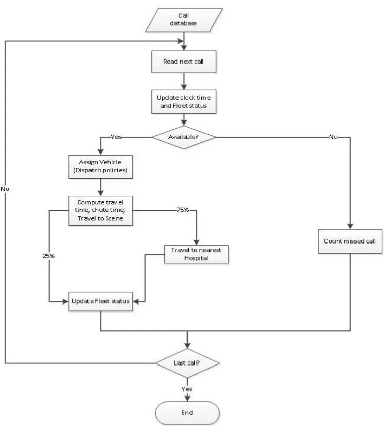
We developed the simulation module using Java (SE Version 7). The simulation module is de-signed to run a trace-driven simulation where the calls used in the simulation are read from a file. As mentioned above in the call data files each call has a time stamp, location, priority, and ser-vice time information. This approach is beneficial for testing and model validation as well as for comparing various dispatch policies. The main logic flow of the simulation model begins with a 9-1-1 call read from a file. The program updates all vehicles’ information including current location and status (idle or busy). Then based on the status and location of vehicles, as well as priority and location of this new incoming call, the program decides which vehicle(s) to dispatch according to the dispatch policy applied. If there is no vehicle available, then the program counts this call as a missed call. Once an ambulance is assigned to a call its status is set to busy, after a short time of preparation (chute time) it departs to the incident scene. Next, we calculate the distance to incident followed by the travel time using the regression models developed earlier. When the vehicle reaches the scene, some form of on-scene treatment is provided to the patient. In our apriori generated call datasets about 75% of the incidents require more than 15 minutes of service time which we assume they require transport to the nearest hospital. The travel time to the nearest hospital is calculated by the corresponding regression models discussed earlier. If transportation to hospital is not needed (service time less than 15 min.) then the call is com-pleted at the scene and the ambulance becomes available for the next call. The ambulance could be assigned to the next call after service completion at the scene or at the hospital or enroute to their next post or base. If it is not assigned to a new call, then it returns to its base station or post and waits for the next dispatch order. To the best of our knowledge, no previous model included enroute dispatch. A high-level flowchart of the dispatch process is depicted in Figure 1.
4 THE SEARCH ALGORITHM
In order to determine the initial ambulance posts (locations) we developed a tabu search (TS) al-gorithm. Since our aim is to test the efficacy of a tiered dispatch policy on multiple call types, we adopted the novel objective function develop by Knight et al. [15] that combines heterogeneous outcome measures into a single function as the fitness function of the TS algorithm.
Figure 1– Simulation model overview flow chart.
406
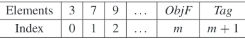
BALANCING AMBULANCE CREW WORKLOADS VIA A TIERED DISPATCH POLICYElements 3 7 9 . . . ObjF Tag
Index 0 1 2 . . . m m+1
Figure 2– Array representation of a solution.
The basic operation in the TS involves moving an ambulance from nodeito nodej, where nodej is the best location in the neighborhood. We defined the neighborhood as the nodes immediately surrounding the selected node. A chief mechanism for exploiting memory in tabu search is to declare a subset of solutions similar to recently examined solutions are tabu. Each tabu has a tenure (duration) which determines how many iterations the tabu be in effect. The tabu list also referred to memory comprises of solutions (tabu) previously visited. The size of the tabu list equals the tenure of tabu because once a tabu passes tenure it will be automatically removed from the tabu list (memory). Tabu list size and tenure also define the maximum number of tabus allowed at any time. However in TS algorithm we need to consider how to design tabu so that the algorithm won’t move to a solution state previously visited. We use the locations of all response ambulances’ posts i.e. the solution vector’s previous m elements as tabu because the solutions are distinguished by the ambulance locations. In order not to repeat any previous accepted solution, we set tabu list size to the number of iterations.
The majority of the existing objective functions in EMS literature are based on single aspect of EMS, e.g., coverage or cardiac arrest survivability function. As previously noted, to capture the different types of calls and their different level of interests to EMS administration, we adopted Knight et al.’s objective function [15] as the fitness function of our TS:
Ob j F(state)=w0S F(RT)+w1CV1(RT)+w2CV2(RT)+w3CV3(RT) (1)
S F(RT)=1/1+exp(−0.26+0.139RT) (2) where S F is a survival probability function for OHCA patients shown in Eq. (2), CV de-notes a function which tallies the number covered calls for priority 1, 2 and 3 calls under a pre-determined RT threshold. We follow Knight et al.’s heterogeneous measures and set w0 = 16, w1 =8,w2= 2,w3 = 1 for OHCA-, priority 1-, priority 2-, and priority 3-calls, respec-tively. The correspondingCV functions with the target RTs in minutes are shown in Eqs. (3-5):
CV1(RT)=
1 0≤ RT ≤8
0 RT >8 (3)
CV2(RT)=
1 0≤RT ≤14
0 RT >14 (4)
CV3(RT)=
1 0≤RT ≤21
0 RT >21 (5)
We note that in practice the EMS administrators can easily modify the fitness function and the weights chosen in this paper to accommodate their priorities.
5 NUMERICAL EXPERIMENTS
In order to test the efficacy of the proposed tiered dispatch policy on ambulance crew work-loads and the resulting OHCA survival rates, response times per call priority we applied our simulation-optimization approach to the 84 problem instances generated from the real data de-scribed in Section 3. It is important to note that in our approach the fleet size is an input vari-able which clearly impacts the average workload of the deployed ambulances where low fleet sizes will result in high workloads and vice versa. Since we are using the same data set used by Rajagopalan et al. [40] initially we adapted the fleet sizes prescribed (recommended) by their dynamic expected coverage location (DECL) model which finds the minimum of ambulances to meet the target coverage rate. We noticed that with the DECL prescribed fleet sizes for the 84 problems instances, when we run the simulation optimization model with defaults dispatch pol-icy, the resulting average ambulance workload is about 54-56% which is considered high in the EMS community. Hence, we conducted some experiments for each of the 84 problem instances to determine the fleet sizes which will result in 30-32% average workload so that we can test the efficacy of the tiered dispatch policy under high and low average workloads. The fleet sizes for high- and low-average workloads are shown in Table 1. Thus, two dispatch policies and two sets of fleet sizes give us a total of four different settings for each of the 84 problem instances which lead to 4×84=336 runs.
Table 1– Fleet sizes for high (H) and low (L) average workload by time of the day and day of the week.
Interval Monday Tuesday Wednesday Thursday Friday Saturday Sunday
H L H L H L H L H L H L H L
12 am – 2 am 11 15 14 21 13 19 14 19 15 20 19 24 17 27
2 am – 4 am 13 19 14 19 13 18 13 20 14 18 15 23 16 26
4 am – 6 am 12 15 13 14 12 15 13 15 14 16 13 18 13 19
6 am – 8 am 15 23 16 22 15 22 15 22 15 22 13 19 13 18
8 am – 10 am 17 29 18 30 17 31 17 30 18 29 16 25 15 24
10 am – 12 pm 19 34 19 33 17 33 18 33 19 33 18 29 17 28
12 pm – 2 pm 19 34 19 33 18 35 19 34 19 34 19 32 18 30
2 pm – 4 pm 19 36 19 33 19 33 18 34 19 36 18 32 18 31
4 pm – 6 pm 18 37 19 35 18 35 18 35 19 38 18 32 16 29
6 pm – 8 pm 17 35 19 33 16 31 16 32 17 32 18 33 16 30
8 pm – 10 pm 16 28 16 29 15 29 16 29 17 32 18 31 16 29
10 pm – 12 am 14 25 16 26 14 24 14 25 17 30 17 32 15 25
408
BAL AN C IN G AM BU L AN C E C R EW W O R KL O AD S VI A A T IER ED D ISP A T C H PO L IC YTable 2– Monday’s results from high average workload and DEF policy.
Monday High Workload Default Dispatch Policy
Intervals OBJ-Fun OHCA P1 P2 P3 Workload
Exp. Saved Total SF(%) Covered Total % Covered Total % Covered Total % AVG STD MIN MAX Range
12 am – 2 am 967.09 1.506 3 50.19 58 97 59.79 216 274 78.83 47 54 87.04 0.401 0.060 0.246 0.482 0.237
2 am – 4 am 926.98 1.499 3 49.95 51 77 66.23 225 249 90.36 45 50 90.00 0.453 0.104 0.196 0.606 0.410
4 am – 6 am 718.88 0.993 2 49.63 39 58 67.24 178 200 89.00 35 35 100.00 0.386 0.097 0.229 0.544 0.315
6 am – 8 am 1431.86 1.491 3 49.70 92 141 65.25 303 365 83.01 66 75 88.00 0.482 0.051 0.377 0.569 0.192
8 am – 10 am 1791.10 2.006 4 50.16 103 199 51.76 416 525 79.24 103 118 87.29 0.588 0.065 0.466 0.697 0.230
10 am – 12 pm 2314.77 3.048 6 50.81 145 244 59.43 496 621 79.87 114 139 82.01 0.606 0.069 0.455 0.746 0.291
12 pm – 2 pm 2131.61 2.038 6 33.96 128 238 53.78 477 608 78.45 121 136 88.97 0.605 0.074 0.459 0.718 0.259
2 pm – 4pm 2217.16 3.010 6 50.17 137 247 55.47 479 627 76.40 115 139 82.73 0.641 0.062 0.507 0.742 0.235
4 pm – 6 pm 2101.70 2.544 6 42.40 129 247 52.23 461 629 73.29 107 139 76.98 0.659 0.067 0.538 0.777 0.239
6 pm – 8 pm 1831.67 2.042 4 51.04 108 209 51.67 416 541 76.89 103 120 85.83 0.621 0.074 0.472 0.717 0.245
8 pm – 10 pm 1541.44 1.528 3 50.92 91 169 53.85 353 448 78.79 83 98 84.69 0.554 0.073 0.403 0.714 0.311
10 pm – 12 am 1360.39 1.524 3 50.80 84 138 60.87 299 364 82.14 66 75 88.00 0.525 0.081 0.325 0.623 0.298
Sum 23.228 49 Avg= 58.13 80.52 86.80 0.543 Avg= 0.389 0.661 0.272
XU
N
L
I
a
n
d
C
EM
SA
YD
AM
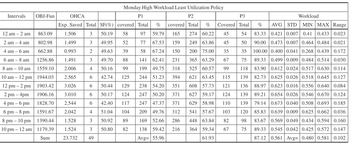
Table 3– Monday’s results from high average workload and LU policy.
Monday High Workload Least Utilization Policy
Intervals OBJ-Fun OHCA P1 P2 P3 Workload
Exp. Saved Total SF(%) covered Total % covered Total % Covered Total % AVG STD MIN MAX Range 12 am – 2 am 863.09 1.506 3 50.19 58 97 59.79 165 274 60.22 45 54 83.33 0.421 0.007 0.41 0.433 0.023
2 am – 4 am 802.98 1.499 3 49.95 52 77 67.53 159 249 63.86 45 50 90.00 0.473 0.007 0.464 0.484 0.021 4 am – 6 am 662.88 0.993 2 49.63 39 58 67.24 150 200 75.00 35 35 100.00 0.400 0.041 0.268 0.439 0.172 6 am – 8 am 1256.86 1.491 3 49.70 88 141 62.41 231 365 63.29 67 75 89.33 0.499 0.009 0.484 0.514 0.030 8 am – 10 am 1559.10 2.006 4 50.16 99 199 49.75 318 525 60.57 99 118 83.90 0.612 0.024 0.517 0.630 0.114 10 am – 12 pm 1944.03 2.565 6 42.74 125 244 51.23 394 621 63.45 115 139 82.73 0.625 0.026 0.518 0.645 0.127 12 pm – 2 pm 1903.42 3.026 6 50.44 129 238 54.20 351 608 57.73 121 136 88.97 0.623 0.016 0.556 0.640 0.084 2 pm – 4pm 1906.16 3.010 6 50.17 124 247 50.20 371 627 59.17 124 139 89.21 0.654 0.026 0.546 0.670 0.124 4 pm – 6 pm 1828.70 2.544 6 42.40 117 247 47.37 371 629 58.98 110 139 79.14 0.673 0.040 0.508 0.693 0.185 6 pm – 8 pm 1591.67 2.042 4 51.04 104 209 49.76 312 541 57.67 103 120 85.83 0.639 0.009 0.625 0.662 0.036 8 pm – 10 pm 1390.44 1.528 3 50.92 89 169 52.66 286 448 63.84 82 98 83.67 0.569 0.049 0.434 0.594 0.160 10 pm – 12 am 1179.39 1.524 3 50.80 82 138 59.42 216 364 59.34 67 75 89.33 0.545 0.042 0.425 0.572 0.147 Sum 23.732 49 Avg= 55.96 61.93 87.12 0.561 Avg= 0.480 0.581 0.102
a
O
per
ac
ional,
V
ol.
36(
3)
,
410
BALANCING AMBULANCE CREW WORKLOADS VIA A TIERED DISPATCH POLICYColumns “P1-P3” display the number of priority 1-3 calls reached under the corresponding tar-get RT, total number of priority 1-3 calls, and the resulting coverage statistics in percentage. Column “Workload” displays the workload statistics (average, standard deviation, minimum, maximum, and range). For example in Table 2 row 12 a.m. – 2 a.m. we display the results from applying the default dispatch policy with DECL prescribed fleet size of eleven ambulances. The results show that the average workload is 0.401 and the range is[0.246−0.482]. There are 3 OHCA calls and the expected number of OHCA survivors based on the realized RTs is 1.506 and the resulting average survival probability is 50.19%. How we track the OHCA calls is an important real-life feature of our model. As mentioned earlier about 0.5% of all calls tends to be confirmed OHCA. Since an OHCA incident triggered call must be priority 1 call and given the percentage of priority 1 call is 23.23%, in our trace-driven simulation the percentage of OHCA incidents among priority 1 calls is 2.15%. For example, in this time interval, there were a total of 428 calls from which 100 calls are randomly sampled as priority 1, 274 calls are randomly sampled as priority 2, 54 calls are randomly sampled as priority 3 using 23.23%, 63.13% and 13.64%, respectively. From the sampled 100 priority 1 calls, 3 calls are categorized as OHCA using 2.15%. We analyzed the findings for each day, conducted a series of pairedt-tests to de-termine whether there is a significant difference between the average values of each of the key performance metrics (OHCA survival probability, coverage rates by call priority, and workload range). We found that the test results are consistent across the days of the week. Thus, hereafter we will use Monday’s results to summarize the results of the experiments.
5.1 OHCA Survival Probability and Priority 1 Call Coverage Comparisons
We are primarily interested in the magnitude of the difference between the mean OHCA survival probabilities resulting from the default dispatch policy (DEF), and the alternate dispatch policy of LU; and, further, whether or not this difference is statistically significant. Similarly, we are interested in differences in the mean coverage rates of the dispatch policies. For brevity, we formally state the null and alternate hypotheses for the OHCA survival probability as follows:
• H0: The difference in the mean OHCA values under DEF and LU policies is zero. • H1: The difference in the mean OHCA values under DEF and LU policies is greater than
zero.
Table 4, below, summarizes the results of the 20 pairedt-tests of Monday’s runs.
Under high average workload conditions, we note that the mean difference in OHCA survival probability between DEF and LU is –0.0070. While this implies that, on Mondays, the LU policy improves OHCA survival probability by 0.7%, it is clearly statistically insignificant (p-value =0.33). Importantly, across all days, we note nearly identical results where the mean differences range from –0.0102 (Sunday) to 0.0227 (Wednesday) with all statistically insignificant (1-tail, 5% significance level).
Table 4– Summary of pairedt-test results.
Mean Difference
High Average Workload Low Average Workload
DEF – LU DEF – LU
Diff. P-value Diff. P-value
OHCA –0.0070 0.33* 0.0000 NA
P1 Coverage 0.0217 <0.01 0.0491 <0.01 P2 Coverage 0.1860 <0.01 0.2670 <0.01
P3 Coverage –0.0033 0.34* 0.0034 0.12*
WL range 0.1699 <0.01 0.3103 <0.01
Under low average workload conditions, the mean difference in OHCA survival probability be-tween DEF and LU policies is zero for all days. This is, in fact, an expected result. The system wide ambulance busy probability is in the neighborhood of 30% since both dispatch policies send the nearest ambulance to OHCA calls, probability of finding an idle ambulance nearby is thus much greater than it would be in systems where the average busy probability is high.
The null and alternate hypotheses for priority 1 call coverage are as follows:
• H0: The difference in the mean priority 1 call coverage values under DEF and LU policies is zero.
• H1: The difference in the mean priority 1 call coverage values under DEF and LU policies is greater than zero.
Under high workload conditions, the mean difference in priority 1 call coverage between DEF and LU is seen to be (Table 4) 0.0217, and is statistically significant at theα=0.01 level. Across all days, we note similar results, i.e., that the difference is statistically significant atα = 0.01 except for Thursdays at theα=0.05 level. We also note that the differences range from 0.0206 (Thursday) to 0.0414 (Sunday). Under low average workload conditions, we see nearly identical results where the mean differences range from 0.0477 (Sunday) to 0.0620 (Wednesday), with all statistically significant (1-tail, 1% significance level).
These results suggest that the default and alternative dispatch policy have different priority 1 call coverage values. The former thus achieves 2.06% to 4.14% more coverage under high workload conditions, and 4.77% to 6.20% more coverage under low workload conditions than does the latter.
5.2 Priority 2 and 3 Call Coverage Comparisons
Utilizing similar forms from earlier comparisons, the null and alternate hypotheses for priority 2 call coverage are as follows:
412
BALANCING AMBULANCE CREW WORKLOADS VIA A TIERED DISPATCH POLICY• H1: The difference in the mean priority 2 call coverage values under DEF and LU policies is greater than zero.
Referring again to Table 4, we find that, under high workload conditions, the mean difference in priority 2 call coverage between DEF and LU is 0.1860. This implies that, on Mondays, the DEF policy achieves 18.6% more coverage for priority 2 calls. The p-value is less than 0.01. We thus reject the null hypothesis that the two policies have same mean coverage at theα = 0.01 significance level. Across all days, we note identical results, where the mean differences range from 0.1699 to 0.1992 and, again, all are statistically significant at the 1% single-tail significance level. Under low workload conditions, the mean differences range from 0.2649 to 0.276, where, again, all are statistically significant at the 1% significance level. The null and alternate hypotheses for priority 3 call coverage are as follows:
• H0: The difference in the mean priority 3 call coverage values under DEF and LU policies is zero.
• H1: The difference in the mean priority 3 call coverage values under DEF and LU policies is greater than zero.
Under high average workload conditions, Table 4 results show that the mean difference in prior-ity 3 call coverage between the two policies is –0.0033 (–0.3%). This implies that, on Mondays, the LU policy results in a slightly higher priority 3 call coverage. However, the one tailt-test critical value is 0.34, which allows acceptance of the null hypothesis, H0.
Examining other days, we find the same results, except that on Saturdays, a small, statistically significant (P-value = 0.025) difference (1.45%) occurs in favor of the DEF policy. Again, though, on all other days, the mean difference is not statistically significant.
Under low average workload, the results are similar to those for high workload conditions. Thus, with the exception of Tuesday’s results, where the mean difference is quite minimal (0.64%) but statistically significant (P-value=0.038), the mean difference on all other days was found to be not statistically significant. Hence, we can safely conclude that coverage of priority 3 calls under LU policy will not result in a significant reduction under either high- or low-workload conditions. This is a finding of some practical and theoretical importance.
5.3 Workload Imbalance Comparisons
Workload rangereflects the degree to which the workload is balanced/imbalanced across all ambulances. If, for example, the workload range is 0.20, it means that the difference between the busiest and least busy ambulance is net 10% (e.g., 0.43 and 0.23). It is an important metric that adds to the information needed by administrators in order to create a more efficient and effective fleet of ambulances. We follow a similar procedure to test themeandifference of workload be-tween the various dispatch policies. According to the design ofleast utilization dispatch policy
described previously, we expect to see LU reduce the workload range considerably more relative to DEF. We formally state the relevant null and alternative hypotheses below:
• H0: The difference in the mean workload ranges under DEF and LU policies is zero.
• H1: The difference in the mean workload ranges under DEF and LU policies is greater than zero.
As shown in Table 4, under high workload conditions the difference of mean ranges between DEF and LU is 0.1699 (16.99%) which is statistically significant at the 1% significance level. As anticipated, the latter reduced the workload imbalance from 27.18% to 10.19%, representing a sizeable 62.51% reduction in magnitude. Further, across all days, we note significant reduc-tions in workload imbalance where the mean differences ranges from 0.1441 to 0.2109, with all statistically significant (1-tail 1% significance level).
Of note, we observe a larger reduction in imbalances under low workload conditions where Monday’s results show a difference of 0.3103 (31.03%). Essentially, LU policy reduced the im-balance from 0.4242 to 0.1138, representing a 73.20% reduction. Not surprisingly, at-test shows this reduction to be statistically significant at the 1% level. Similarly, across all days, the mean differences ranges from 0.2662 to 0.3389, where, again, all are statistically significant (1-tail 1% significance level).
5.4 Overall Comparisons
From previous sub-sections, we see that neither DEF nor LU is likely to make a statistically significant difference in terms of the OHCA survival rate or priority 3 call’s coverage. For the coverage of priority 1 calls, excluding OHCA, DEF is statistically better than LU; but, the magni-tude of this difference is rather small. For instance, under high workload conditions on Mondays, DEF provides coverage of 58.13% of priority 1 calls, while LU offers coverage of 55.96%. For coverage of priority 2 calls, the difference between DEF and LU is statistically significant. For instance, under high workload conditions on Mondays, DEF has coverage of 80.52% of priority 2 calls, while LU generates only 61.93% coverage. In terms of coverage of priority 1 (excluding OHCA) calls, DEF thus provides slightly better performance than does LU. In cover-ing priority 2 calls, DEF is considerably better than LU. Interestcover-ingly, however, is the fact that, for the workload range, LU achieves significantly better outcomes than does DEF. For instance, under high workload conditions on Mondays, LU reduces the workload from DEF’s 0.2718 to 0.1019, a notable reduction of 62.51%.
414
BALANCING AMBULANCE CREW WORKLOADS VIA A TIERED DISPATCH POLICYpriority 1 calls) OHCA calls. Lastly, the OHCA survival probability is a continuous function based on RT. When an OHCA RT is, say 8 minutes 1 second vs. 8 minutes, the difference in the computed survival probability is the difference 0.2990−0.2985 = 0.0005, clearly negligible. Taken all together, mean difference in OHCA survival probability between DEF and LU is, as expected, negligible. However, none-OHCA priority 1 calls hold the second largest weight and they are also being covered with the nearest ambulances. The results show that LU policy tends to cover 2-4% less than DEF policy and the difference is statistically significant. We believe that this difference is in part due to the simple 0/1 tally function used in the objective function (as well as widely in the literature) where a RT of 8 minutes counts towards being the covered (1), conversely an RT of 8 minutes 1 second will not count at all (0). Further, as noted in Section 1, outside the OHCA incidents there appears to be no clear connection between fast RTs and patient outcomes. Therefore, we can argue that 2-4% less coverage of non-OHCA P1 calls do not necessarily imply any reduction in patient survival.
Interestingly, DEF and LU lead to significantly different coverages of priority 2 calls since the former, unlike the latter, chooses to send its nearest ambulance to priority 2 calls. This generally results in less travel time and, hence, a shorter RT. Curiously, it is not entirely clear why there is little or no difference between the two policies in terms of priority 3 call coverage. One possible explanation is that the target RT of priority 3 coverage of 24 minutes is not difficult to meet, even if the nearest ambulance is not dispatched. The alternative dispatch policy was designed to favor sending less busy vehicles from all those available so it reduces the workload range significantly relative to DEF.
6 CONCLUSIONS AND FUTURE RESEARCH
In this paper we developed a simulation embedded optimization approach to relocate ambulances and determine flexible dispatch policies for maximum performance. The proposed approach is based on a thorough analysis of a large historical dataset which makes the model and outcomes more realistic.
In particular, we considered various call priorities; modeled distribution and travel time based on historical data analysis; compared selected dispatch policies; and, then, developed weighted objective functions for multiple classes of concerned interests. In addition, in our trace-driven simulation model, we included enroute dispatching in which ambulances can be dispatched to the next call when one completes a previous call regardless of its current location. Thus, we were able to mimic key real-life conditions of EMS operations.
In order to capture different types of calls and their different level of interests to EMS admin-istration we adapted Knight et al.’s objective function which combines heterogeneous outcome measures into a single function that takes four types of calls into consideration. The objective function was able to capture a variety of phenomena of interest to EMS administrators, while providing sufficient flexibility for them to create their own ‘best’ objective function. In this
gard, we applied two dispatch policies (DEF and LU) in an effort to examine how various policies might affect the performance of an EMS system.
We ran our simulation model for seven days, creating 12 time intervals within each day under both high and low workload conditions. Results suggest that there is little or no difference be-tween DEF and LU in terms of OHCA survival rate and priority 3 call coverage. DEF achieves higher coverage of priority 2 calls than does LU. Although DEF tends to have better perfor-mance in its coverage of priority 1 calls, the difference is rather small and in all likelihood does not impact patient outcomes. On the other hand LU significantly reduced the workload range which suggests that it can help balance the workload amongst ambulances and potentially have a positive impact on quality of medical care delivered by the crews.
In general, there appears to be some benefits to practicing DEF or LU dispatch policy. We are able offer some guidelines. For example, if an EMS administrator is concerned more about strict call coverage versus workload balance of ambulance crews, he/she should probably favor the default dispatch policy that sends the nearest ambulance to all calls. On the other hand, if he/she seeks a more balanced workload amongst vehicles, LU policy is clearly more appropriate. However, should an EMS agency adopt a tiered dispatch policy similar to LU they should monitor RTs and patient outcomes as well as keeping track of coverage statistics which are the industry norm. We have thus demonstrated that our proposed approach can be used by EMS managers to evaluate their current practices and test the efficacy of alternate policies.
Although the findings are promising there are some certain limitations of our approach. For ex-ample, the simulation-optimization model can be applied in a true GIS environment utilizing the real road network, including one-way streets which will further increase its realism and useful-ness. Ambulance travel models can also be improved by taking into account the traffic conditions which vary especially during the rush hours as well as weather conditions.
In terms of future research, there are a number of possible directions. The approach can be extended to consider optimal time of base (post) swaps for the busiest and least busy pairs of ambulances in order to balance their workloads, while dispatching the closest unit to priority 1 and 2 calls. Another extension of the base simulation-optimization model can be to include a two-tiered response where fire engines with EMTs are dispatched to priority 3 calls and ambu-lances are dispatched to priority 1 and 2 calls. After EMTs assess the patient’s condition they can request an ambulance for transport to a hospital. Finally, our simulation optimization model can be extended to study emergency room crowding and ambulance diversion policies [19].
ACKNOWLEDGMENTS
416
BALANCING AMBULANCE CREW WORKLOADS VIA A TIERED DISPATCH POLICYREFERENCES
[1] TORO-D´IAZHET AL. 2013. Joint location and dispatching decisions for Emergency Medical Ser-vices.Computers & Industrial Engineering,64(4): 917–928.
[2] ANDERSSONT & VARBRANDP. 2007. Decision support tools for ambulance dispatch and reloca-tion.Journal of the Operational Research Society,58(2): 195–201.
[3] HENDERSONSG. 2011. Operations research tools for addressing current challenges in emergency medical services, in Wiley Encyclopedia of Operations Research and Management Science, J.J. COCHRAN, Editor, John Wiley & Sons, Inc.: Hoboken, NJ.
[4] INGOLFSSONA. 2012. EMS Planning and Management, in Operations Research and Health Care Policy, G. ZARIC, Editor, Springer.
[5] MASONAJ. 2013. Simulation and real-time optimised relocation for improving ambulance opera-tions, in Handbook of Healthcare Operations Management: Methods and Applications. B. DENTON, Editor, Springer: New York. p. 289–317.
[6] MCLAYL & MAYORGAM. 2010. Evaluating emergency medical service performance measures. Health Care Management Science,13(2): 124–136.
[7] GOLDBERGJB. 2004. Operations Research Models for the Deployment of Emergency Services Ve-hicles.EMS Management Journal,1(1): 20–39.
[8] DEMAIOVJET AL. 2003. Optimal defibrillation response intervals for maximum out-of-hospital cardiac arrest survival rates.Annals of Emergency Medicine,42(2): 242–250.
[9] PONSPTET AL. 2005. Paramedic response time: does it affect patient survival? Academic Emer-gency Medicine,12(7): 579–676.
[10] BLACKWELLTHET AL. 2009. Lack of association between prehospital response times and patient outcomes.Prehospital Emergency Care,13(4): 444–450.
[11] BLANCHARDIE ET AL. 2011. Emergency Medical Services Response Time and Mortality in an Urban Setting.Prehospital Emergency Care,16(1): 142–151.
[12] WEISSSET AL. 2013. Does Ambulance Response Time Influence Patient Condition among Patients with Specific Medical and Trauma Emergencies?Southern Medical Journal,106(3): 230–235.
[13] BOERSMAEET AL. 1996. Early thrombolytic treatment in acute myocardial infarction: reappraisal of the golden hour.The Lancet,348(9030): 5.
[14] RAGONEMG. 2011. Are we ready for the future? Where EMS stands now & where it’s prepared to go.Journal of Emergency Medical Services,36(2): 38–43.
[15] KNIGHT VA, HARPER PR & SMITHL. 2012. Ambulance allocation for maximal survival with heterogeneous outcome measures.Omega,40(6): 918–926.
[16] BROTCORNE L, LAPORTE G & SEMET F. 2003. Ambulance location and relocation models. European Journal of Operational Research,147(3): 451–463.
[17] FARAHANIRZET AL. 2012. Covering problems in facility location: A review.Computers & Indus-trial Engineering,62(1): 368–407.
[18] LIXET AL. 2011. Covering Models and Optimization Techniques for Emergency Response Facility Location and Planning: A Review.Math. Meth. Oper. Res.,74(3): 281–310.
[19] ARINGHIERIRET AL. 2016. Emergency Medical Services and beyond: Addressing new challenges through a wide literature review.Computers & Operations Research,59: 349–368.
[20] CARTERGM CHAIKENJM & IGNALLE. 1972. Response Areas For Two Emergency Units. Oper-ations Research,20(3): 571–594.
[21] PERSSEDEET AL. 2003. Cardiac arrest survival as a function of ambulance deployment strategy in a large urban emergency medical services system.Resuscitation,59(1): 97–104.
[22] MCLAYLA & MAYORGAME. 2011. Evaluating the impact of performance goals on dispatching decisions in emergency medical service.IIE Transactions on Healthcare Systems Engineering,1(3): 185–196.
[23] BANDARAD, MAYORGAME & MCLAYLA. 2012. Optimal dispatching strategies for emergency vehicles to increase patient survivability.International Journal of Operational Research,15(2): 195– 214.
[24] MCLAY LA & MAYORGAME. 2013. A dispatching model for server-to-customer systems that balances efficiency and equity.Manufacturing and Service Operations Management,15(2): 205–220.
[25] MCLAYLA & MAYORGAME. 2013. A model for optimally dispatching ambulances to emergency calls with classification errors in patient priorities.IIE Transactions,45(1): 1–24.
[26] BANDARAD, MAYORGAME & MCLAYLA. 2014. Priority Dispatching Strategies for EMS Sys-tems.Journal of the Operational Research Society,65(4): 572–587.
[27] SUDTACHATK, MAYORGAME & MCLAY LA. 2014. Recommendations for dispatching emer-gency vehicles under multitiered response via simulation.International Transactions in Operational Research,21(4): 581–617.
[28] SAVASES. 1969. Simulation and Cost-Effectiveness Analysis of New York’s Emergency Ambulance Service.Management Science,15(12): 20.
[29] HAGHANIA, TIANQ & HU H. 2004. Simulation Model for Real-Time Emergency Vehicle Dis-patching and Routing.Journal of the Transportation Research Board,1882: 176–183.
[30] RESTREPOM, HENDERSONSG & TOPALOGLUH. 2009. Erlang loss models for the static deploy-ment of ambulances.Health Care Management Science,12: 67–79.
[31] MAXWELLMSET AL. 2010. Approximate Dynamic Programming for Ambulance Redeployment. INFORMS Journal on Computing,22(2): 266–281.
[32] YUEY, MARLAL & KRISHNANR. 2012. An Efficient Simulation-Based Approach to Ambulance Fleet Allocation and Dynamic Redeployment. In: Proceedings of the National Conference on Artifi-cial Intelligence, p. 398–406.
[33] SHANE G & HENDERSONAJM. 1999. Estimating Ambulance Requirements in Auckland, New Zealand.Proceedings of the 31st conference on Winter simulation: Simulation – a bridge to the future,2: 1670–1674.
[34] SHANEG & HENDERSONAJM. 2004. Ambulance service planning: simulation and data visual-ization, in Operations Research and Health Care: A Handbook of Methods and Application, Kluwer Academic Publishers. p. 77–102.
418
BALANCING AMBULANCE CREW WORKLOADS VIA A TIERED DISPATCH POLICY[36] ABOUELJINANEL, SAHINE & JEMAIZ. 2013. A Review on Simulation Models Applied to Emer-gency Medical Service Operations.Computers & Industrial Engineering,66(4): 734–750.
[37] GELLERTWET AL. 1989. The VNR Concise Encyclopedia of Mathematics, New York: Van Nos-trand Reinhold.
[38] SHAHIDRET AL. 2009. Comparison of distance measures in spatial analytical modeling for health service planning.BMC Health Services Research,9(1): 1–14.
[39] INFINGERAEET AL. 2013. Increasing Cardiac Arrest Survival by Using Data & Process Improve-ment Measures. JEMS.
[40] RAJAGOPALANHK ET AL. 2011. Ambulance deployment and shift scheduling: an integrated ap-proach.Journal of Service Science and Management,1(4): 66–78.
[41] GLOVERF. 1986. Future paths for integer programming and links to artificial intelligence.Computers & Operations Research,13: 533–549.
[42] JARVISJP. 1985. Approximating the equilibrium behavior of multi-server loss systems.Management Science,31(2): 235–239.
APPENDIX
The dynamic available coverage location (DECL) model proposed by Rajagopalan, Saydam, et al. [40] determines the minimum number of ambulances and their locations to meet a system wide coverage requirement for each time interval. The authors utilize Jarvis’ hypercube approximation algorithm [42]. An added advantage of Jarvis’ methodology is that it allows for server specific general service time distributions which in this study we found that they are normally distributed. Lettbe the index of time intervals,hj,tbe the fraction of demand at node j at time intervalt,n be the number of nodes in the system, andct be the minimum expected coverage requirement at timet. Let pk,t be the busy probability of thekt h preferred server for a given demand node at time intervalt,ρtbe the average system busy probability at time intervalt,mbe the total number of servers available for deployment, and setNjis the set of all servers that can cover node j. The main decision variable is defined as follows:
xj,k,t =
1 if serverkis located at node jat timet 0 if not
yj,k,t =
1 if node j is covered by serverkduring time intervalt 0 if not
Minimize: Z = T
t=1
n
j=1
m
k=1
xj,k,t (9)
Subject to: m
k=1
xj,k∈Nj,t =
m
k=1
yj,k,t ∀j,t (10)
n
j=1
m
k=1
(Z, ρt,k−1)hj,tyk,j,t(1−ρk,t) k−1
l=1
ρl,t ≥ct (11)
n
j=1
m
k=1
xj,k,t ≤m ∀t (12)
yk,j,t,xj,k,t = {0,1} ∀i,j,k,t (13)