An Mathematical Introduction to Population Dynamics

(1)

An Mathematical Introduction to Population Dynamics

UNDER CONSTRUCTION

Howie Weiss

Georgia Tech

(2)

Introduction

c

2010 Howard Weiss

1.1 About these lectures

These lecture notes follow the introductory course on mathematical biology that I teach at Georgia Tech. My students come from all corners of the campus including mathematics, biology, engineering, physics, and computing. The majority of students are conducting thesis research on microbial population dynamics or transmission of infectious diseases, and I try to choose models and applications with this in mind. The stress on population dynamics is not a large restriction since much of biology can be viewed as the study of populations. This includes areas such as cancer biology, cell biology, conservation biology, demography, developmental biology, ecology, epidemiology, evolutionary biology, genetics, immunology, infectious diseases, neuroscience, parasitology, wildlife biology, etc. Also, even though this is not their current research focus, most students are also interested in applications of mathematical modeling to biodiversity and conservation biology, and I introduce the main modeling tools used in these areas.

My goals are to introduce and rigorously analyze the most commonly used population and infectious disease transmission models, so that at the end of the semester the students can formulate and analyze their own population models, and navigate the literature. Our modeling philosophy follows Levins (taught to me by the apostle Levin), where models generate hypotheses and provide a framework for the design and interpretation of empirical studies and generalize on their results. Practically, models provide a way to design and evaluate protocols for epidemiological and clinical interventions. We do not present predictive (precise) models.

Along the way I try to succinctly present the key biological ideas and compare the predictions of models with actual lab or field data. Feedback from my students has been positive, and several students suggested turning my lecture notes into a short monograph. I have also written these notes for mathematicians who are starting to work on some applications to biology and wish to learn the basic population models and how to analyze them.

The minimal course prerequisite is basic knowledge of differential equations, although the ideal prerequisite is a second course in ordinary differential equations (ODEs) or dynamical systems. A few subsections contain stochastic models which require a more substantial mathematical prerequisite. These subsections are independent of the other sections.

Our treatment of population dynamics is significantly more rigorous than is commonly found in textbooks. Some textbooks discuss the local analysis of equilibrium points, fewer discuss bifurcations, and very few discuss

(6)

global properties of the orbit structure. For the latter, most authors follow the geometric approach in [Rosenzweig and MacArthur, 1963] and use null-clines to study the geometry of solutions of systems of two ODEs. Our treatment is considerably more analytical.

At first glance, it may appear that the topics in Chapters2and3(single species and community dynamics) are disjoint from the topics in Chapter 4(disease transmission dynamics). This is definitely not the case. Within an infected host, viruses such as HIV and hepatitis C compete for cells to infect, and on the population level, compete for new hosts to infect [Tillmann et al., 2001]. Hutchinson views competition between species as resulting from niche overlap (3.1.1) and disease ecologists view, say Lyme disease in New York State, as resulting from the niche overlap of the human population, the pathogen population (B. burgdorferi), the vector population (deer ticks), and the reservoir population (white-footed mouse). Although such complex models are beyond the scope of these notes, we present many of the basic components and tools to analyze them.

Finally, the lecture notes contain a small number of exercises. There are two types of exercises, with the distinction more typographical than pedagogical. Some problems are explicitly stated as problems. Others are embedded in the text and are preceded by a diamond symbol♦.

1.2 What is a population and how does it change?

A population is a group of individuals of the same species that occupy a particular area (see [Wells and Richmond, 1995] for13definitions). Changes in population sizes and composition result from interactions between individuals of the same species, interactions between individuals of different species, interactions with the environment, disease, food supply, etc. Interactions can be predatory, cooperative, mutualistic, commensural, etc.. These changes are expressed in terms of birth rates, death rates, immigration rates, and emigration rates. The goals of population dynamics are to understand, explain, and predict the sizes and compositions of populations over time and space.

Populations are controlled by density independent and density dependent regulation. In density independent regulation, mortality or fertility rates are unaffected by population density. Density independent factors include weather, natural catastrophes, food supply, and pollution. A severe flood can just as easily wipe out a large popu-lation as a small one. In density dependent regupopu-lation, mortality or fertility rates depend on the popupopu-lation density through factors such as predation, competition, and infectious diseases. If a population is densely distributed, each individual will have a higher probability of catching an infectious disease than if the individuals had been living farther apart. Sometimes a factor that first appears to be density independent is actually density dependent. If a refuge helps animals survive cold weather, and if there are limited refuges available, then when the population is small, all find refuge and few die, but when the population size is large not all fit into the refuges, and a larger proportion of the population die. There have many discussions in the literature about the relative importance of these two regulatory mechanisms, but now most agree that both play a critical role. This interplay is currently a major theme in population dynamics.

Many researchers date the modern era of population dynamics (sometime called population ecology) to 1798 and the publication by Malthus of his treatise “An Essay on the Principle of Population” [Malthus, 1798]. Malthus believed that human populations grow exponentially while the food supply grows linearly, and fierce competition would naturally ensue. He argued that unless the population is checked by moral restraint or disaster (e.g., disease, famine, or war), widespread poverty and wars would inevitably result.

(7)

1.3. WHY DO BIOLOGISTS NEED MATHEMATICAL MODELS? 7

of the modern theory that we mention during these lectures include Gause, Kermack, McKendrick, Leslie, Lotka, May, MacArthur, Ross, and Volterra.

1.3 Why do biologists need mathematical models?

“Mathematics is biology’s next microscope, only better. Biology is mathematics’ next physics, only better.” Joel Cohen, [Cohen, 2004]

“Doing research in population biology without mathematical and/or computer simulation models is like playing tennis without a net or boundary lines.” Bruce Levin (from the top of his web page, 2009)

A model is a simplification or abstraction of nature, separating the important from the minor and irrelevant. Models are used to approach questions too complex, inaccessible, numerous, diverse, mutable, unique, dangerous, expensive, big, small, slow or fast to approach by other means [McKenzie, 2000].

Utility of mathematical population models

1. Mathematical models help biologists organize their thinking. A biologist could spend a lifetime measuring population sizes and distributions and have no idea about interactions and mechanisms. Models give direction and idea about the important things to measure and provide a means to interpret data.

2. Mathematical models help generate testable predictions. Biologists will make much faster progress toward understanding nature by trying to verify or refute specific predictions, rather than measuring everything without a plan. Models also expose faulty assumptions.

3. Mathematical models help biologists distinguish between different patterns they see in nature and different mechanisms that might cause these patterns. Mathematics is all about identifying and classifying patterns. Thus mathematical models can elucidate biological mechanisms.

4. Mathematical models provide a way to design and evaluate protocols to manage and control animal popu-lations, natural resources (e.g., forests), wildlife resources (e.g., fisheries, deer population), and infectious diseases. Management requires predictions and predictions require models. Mathematical models provided guidance to the British government on controlling their 2001 outbreak of foot and mouth disease. Nobody will be upset if scientists start a smallpox outbreak in a large city and study the efficacy of various control strategies or kill half the female members of a grizzly bear population and measure the population recovery time, if they do so using mathematical models instead of actual populations.

“All models are wrong, but some are useful.” George Box [Box, 1976]

1.4 Limitations of mathematical models

(8)

realism and precision in her model, and can sacrifice generality. It does not matter that her foot and mouth disease model can not be used to control outbreaks of bluetongue. A biologist interested in discovering a general principle such as whether macrophages can limit a bacteria population, requires realism and generality in her model, and can sacrifice precision. A model that is realistic and general is sometimes called a conceptual model. Thus models can be used for general understanding of biological principles or for precise population predictions, but not both. Agent based models are the most precise and realistic, but are the least general.

One must be cautious about going overboard with model realism, even when seeming essential. Imagine devising a population model which is a faithful reflection of an ecosystem in all of its complexity. Any such model would likely require hundreds of nonlinear partial differential equations with time lags, involving hundreds of parameters. Many of these parameters would take years to measure. It may also take many years to develop and implement a reliable computer algorithm to run simulations, and each simulation may require years to run on a super computer. The system may also exhibit chaotic behavior (like for weather forecasting models) that would severely limit the reliability of long term predictions. Clearly a model that is “too realistic” has no practical use.

1.5 Why do mathematicians need population models?

Population dynamics has already generated a considerable amount of new mathematics, and many believe it will be one of the main driving forces of new mathematics during this century.

For one example, the mathematics of nonlinear diffusion equations received much of its impetus from biology. Fisher’s study of the spread of advantageous genes in a population led him to what we now call the reaction diffusion equation with a logistic reaction term. This was simultaneously studied by Kolmogorov et al., who proved the existence of a stable travelling wave of fixed velocity representing a wave of advance of the advantageous gene. Turing also used reaction diffusion equations to understand pattern formation and morphogenesis problems in developmental biology.

In the short and medium term, I believe that population biology will generate many new examples of dynamical systems for mathematicians to study and will provide new questions about both old and new examples. We do not yet know the shape that mathematical biology will take two decades hence, but we recognize some current trends. Among these are the use of multiscale models incorporating diferential equations and stochastic elements, and the ability to identify and classify patterns on many scales within enormous data sets. For the latter problem, innovation and application in other subdisciplines of mathematics, including algebra, geometry, and topology, along with computer science are likely to be essential.

1.6 Confronting models with data

The use of data to evaluate models is fundamental to science. According to Richard Feynmann, “Science is a process for learning about nature in which competing ideas about how the world works [models!] are evaluated against observations.” Unfortunately, long term population and epidemiological data are rare. Few population time series have30generations, although a remarkable exception is the Lenski lab’s long term evolution experiment that recently surpassed50,000 generations of E. coli.

(9)

1.6. CONFRONTING MODELS WITH DATA 9

the field include trapping (mark and recapture), pellet counting, counting vocalizations, fishing catch per effort, percentage ground cover, etc.

1.6.1 Model validation

[Caswell, 1976] argues that model validation is different for a predictive model than for a theoretical (hypothesis generating) model. In a predictive model, “truth” is not the main issue; rather validation involves determining whether the model is acceptable for its intended use, which is usually whether the model mimics some aspect of the real world sufficiently well. In a theoretical model, the focus is on inference about “truth”, and validation focuses on attempts to invalidate the theory [Holling, 1978].

[Zeigler and Oren, 1979] distinguish between types of validity for a predictive model: models that mimic data already acquired and used to parametrize the model, models that accurately reproduce new observed data, and models that not only reproduce observed new data, but truly reflect the way in which the real system operates to produce this behavior (the truth). Although the first type of validity is ubiquitous in the scientific literature, one is actually learning little from such models. According to John von Neumann, “with four parameters I can fit an elephant and with five I can make him wiggle his trunk.” However, if the output of a model does not mimic the data used to parametrize it, then the model is likely to be missing at least one important component. In this sense, a deficient model is more helpful than a model that fits the data.

1.6.2 Model Parameterization

Parametrizing a model from data, or fitting parameters from data, is usually done using the least squares or maximum likelihood methods [Myung, 2003]. The least squares method involves minimizing the difference between the model outputs and the data. More precisely, one tries to minimize, over all values of the parameters, the sum of squares error (SSE) between the data and the model predictions:

SSE(~λ) = N X

i=1

yi−predi(~λ) 2

,

where λ denotes a vector of parameters and predi(~λ)denotes the models prediction for the i−th data point using the parameter setλ.

Given a probability model for the data, the likelihood function is the probability that the model outputs the observed data given a set of parameters. The maximum likelihood method selects the value(s) of the model parameters that make the observed data more likely than any other parameter values. This technique requires maximizing the likelihood function over a high-dimensional space, and a popular algorithm to estimate the maximizer is based on the Markov Chain Monte Carlo (MCMC) simulation method [Diaconis, 2009].

Although in very special cases the two methods produce the same output (e.g., for statistically independent and normally distributed data), in general the two methods produce different parameterizations from the same data set. These days maximum likelihood methods seem much more popular than least squares methods.

There are also Baysian methods of parameter fitting, which allow you to incorporate prior information into the fitting procedure. See [Cooper, 2007] for a short general introduction.

(10)

What does it mean when one model fits the data better than another model, in the sense that the former has a smallerSSE(~λ)or likelihood value? This does not mean that the former model does a better job of capturing the underlying biological process. A good fit is a necessary, but not a sufficient, condition for such a conclusion. This is because a model can achieve a superior fit to its competitors for reasons that have nothing to do with the model’s fidelity to the underlying process.

It is also a good idea to compare a model’s data fitting ability with model variants having a greater number and fewer number of parameters, and with other models in the literature. Model selection tools, such as the Akaike information content (AIC), quantify how well a model fits the data and adds penalties for extra parameters. See [Johnson and Omland, 2004, Wilson, Wilson] for short expositions. Section 4.5 contains an elementary example that clearly illustrates some dangers of overfitting a model.

(11)

Chapter 2

Single Species Models

2.1 Discrete verses continuous population models

Discrete population models are useful when the generations do not overlap or all births occur at fixed intervals. Many insects and annual plants are obvious examples. The Baltimore checkerspot butterfly (state insect of Maryland) breed once per year and lay eggs in early summer. The adults die shortly afterwards, and the eggs hatch into caterpillars in mid summer and re-emerge the next spring as butterflies. The eggs of brown trout in central Pennsylvania streams hatch once per year in the Spring. Moose produce offspring once per year in the Spring. Population models for such animals give rise to difference equations or discrete dynamical systems, which contain a natural time lag. Continuous population models are useful for large populations where births can occur at any time, as with humans.

A system of one or two ODEs is generally easier to analyze than a one-dimensional discrete system. Because of the time lag, a one dimensional discrete model can exhibit complicated dynamics (e.g., chaos). The Poincar´e-Bendixson theorem precludes an autonomous system of one or two ODEs from exhibiting complicated dynamics (see Section 6.3).

2.2 The determinants of population change

There are only four determinants for population change: births (B), deaths (D), immigration (I), and emigration (E). In general, B, I, D, E are functions of population size, time, food availability and quality, environment, etc. For a discrete model, in natural time unitsk, the population at timek+ 1is related to the population at timek

by the following balance equation

N(k+ 1) =N(k) +B+I−D−E. (2.1) For an ODE model, the population change is given by

dN

dt =B+I−D−E. (2.2)

For these lectures, unless otherwise stated, we model closed systems where I=E = 0. A major exception will be our discussion of metapopulations, where births and deaths are ignored, and immigration and emigration are the major players.

(12)

2.2.1 How do microbes reproduce?

Most prokaryotes (bacteria and archaea) reproduce asexually by binary fission, which yields two identical cells in each replicating cycle (see Figure 2.1(a)). This begins when the DNA of the cell is replicated. Each circular strand of DNA then attaches to the plasma membrane. The cell elongates, causing the two chromosomes to separate. The plasma membrane then invaginates and splits the cell into two daughter cells. Binary fission theoretically results in two identical daughter cells, however, the DNA of bacteria has a relatively high mutation rate. Figure 2.1(b) shows E. coli, strain 0157:H7 with different cells in different stages of reproduction.

Similar to more complex organisms, bacteria also have mechanisms for exchanging genetic material (plasmids). Although different from sexual reproduction, the end result is that a bacterium contains a combination of traits from two different parental cells. Three different modes of exchange have thus far been identified in bacteria: transformation, transduction, and conjugation.

Protozoan also reproduce by fission. Most yeasts reproduce asexually by budding, although a few do so by binary fission.

A virus particle or virion is a cellular parasite and can not reproduce without the help of a living cell. To reproduce, a virion binds to the host cell membrane and injects its genetic material (DNA or RNA) into the cell. Once the genetic material has entered the cell, it will hijack the cellular machinery (ribosomes and enzymes) to replicate itself. The newly created viral proteins and nucleic acid combine to form hundreds of new virions. Most viruses exit the cell by making the cells burst, a process called lysis. Other viruses, such as HIV, are released more gently by a process called budding. Unlike bacteria which replicate by producing two cells in each replicating cycle, the replication of viral DNA or RNA is explosive and frequently yields many hundreds of new virions.

Figure 2.1: (a) Bacterial fission [from http://www.uic.edu/classes/bios/bios100/lecturesf04am/binfission.jpg], [b] E. coli strain 0157:H7 [fromci.vbi.vt.edu], (c) Virus reproduction [from mrcovingtonsciencepage.wikis]

2.3 Exponential growth paradigm

The exponential growth model assumes that the birth and death rates are constant, i.e., B = bN, D = dN, where banddare constants. The discrete exponential growth model is

(13)

2.3. EXPONENTIAL GROWTH PARADIGM 13

dN

dt =bN−dN = (b−d)N=rN, (2.4)

where r =b−d. Solving these equations is trivial. In the discrete case, N(k) = (1 +r)k_N_{(0), while for the} ODE, N(t) =N(0) exp(rt). Thus ifb > d the population grows exponentially, if b < d the population decays to zero exponentially, and ifb=dthe population does not change in time. The exponential growth rate ris a common measure of the fitness of the population.

We note that the expressiondN/dt=rN is equivalent toN′

/N =r, and thus the per capita growth rate of the population is constant and equal tor.

The following is a list of major assumptions behind the exponential growth model:

1. The population is closed, i.e., I=E= 0. 2. The ratesb anddnever change.

3. Thus there are no differences in the birth and death ratesbandddue to age, sex, or size. 4. Species exist as single panmictic population (all individuals are potential partners).

5. Reproduction begins immediately after birth (no time lags).

Do some populations grow exponentially? Yes, at least initially. This occurs for species colonizing a new habitat, invasive species when they first arrive, and species that are rebounding from a population crash. Some examples include (notice log scale on y-axis):

1. Inoculation of bacteria into fresh medium after initial lag phase (see Figure 2.2).

2. The invasive Monk parakeet in US 1976-1994 (see Figure 2.3(a)).

3. US population from 1650 to 1800 (see Figure 2.3(b)).

(14)

Figure 2.3: (a) Population of Monk Parakeet in the US during 1976-1992 [Van Bael and Pruett-Jones, 1996] (b) Population of the United States during 1650-1800

(15)

2.3. EXPONENTIAL GROWTH PARADIGM 15

In general, smaller organisms have larger exponential growth rateras illustrated in Figure 2.4

For bacteria transfered from one medium to another, there is an initial lag phase where the individual bacteria are synthesizing RNA, enzymes, and other molecules they need for growth, prior to their resumption of division. Then comes the exponential growth phase (sometimes called the log phase) which is eventually limited by the exhaustion of available nutrients and accumulation of inhibitory metabolites or end products. This phase with slower growth is called the stationary phase. Eventually the bacterial population shrinks, in what is known as the death phase. See Figure 2.5.

Figure 2.5: The four growth phases of bacteria

The efficacy of antibiotics is sometimes growth phase dependent. e.g., Penicillin and other beta-lactam antibiotics are most effective against rapidly growing bacteria.

Through genetic analysis of bacteria during the final stages, we are learning that death allows new life. Since bacteria can evolve in real time, while the vast majority of bacteria are dying, waves of new mutants, which are better and better able to thrive in the noxious and nutrient depleted soup, are thriving [Siegele and Kolter, 1992, Zambrano and Kolter, 1996]. Sometimes this can go on for months.

[Turchin, 2001] has formulated a fundamental law of ecology: a population grows exponentially as long as the environment experienced by all individuals remains constant. Compare Turchin’s statement with Newton’s first law (law of inertia): an object will remain at rest or in uniform motion in a straight line unless acted upon by an external force.

Problem 1. A single cell of the bacterium Escherichia coli, would, under ideal circumstances, divide every twenty minutes. Show that in a single day, one cell of E. coli could produce a super-colony equal in size and weight to the entire planet earth.

Example 1. The Doomsday Population Model, [Cohen, 1995]: The exponential model assumes thatN′

=

rN. Suppose the population growth is even faster and is proportional to the square of the population size, i.e.,N′

=rN2_{. This separable ODE can be easily integrated, and the solution is}

N(t) = N(0)

1−N(0)rt. (2.5)

(16)

2.3.1 Discrete Markov chain model of bacterial growth

We assume that at each time step (generation) a bacterium undergoes binary fission (divides into two cells) with probabilitypand dies with probability1−p, and these are independent of all the other bacteria. LetXk denote the population of generation n. The stochastic process {Xk} is Markov (with a countably infinite state space) since the probability distribution for the population at timen+ 1only depends on the population at timen. Our first goal is to compute the expected valueen=E[Xn]. Assuming thatXn =M, the probability distribution of

Xn+1 is binomial

P(Xn+1= 2k|Xn) =

M k

pk₍₁₋_p₎M−k_. _(2.6) Since the expected value of a binomial random variable with parametersM (number of trials) andp(probability of success) is M p, the conditional expectationE[Xn+1|Xn] = 2pXn. We then use the law of total expectation

E[X] =E[E[X|Y]]to conclude that

E[Xn+1] = 2pE[Xn]. (2.7)

Thus en satisfies the simple difference equationen+1= 2pen, with solution

E[Xn] = (2p)n_m

0. (2.8)

So if p >1/2, the expected population size grows exponentially, and if p <1/2, the expected population size decays to zero exponentially. So far, this is very similar to the behavior of solutions of the deterministic exponential growth model (2.3), where the population size grows exponentially if the birth rate is larger than the death rate, and decays to zero otherwise.

Problem 2. Compute the variance ofXn using the law of total varianceV[X] =E[V[X|Y]] +V[E[X|Y]]. However, unlike the deterministic model, forp > 1/2 there is a positive probability that the population will go extinct. If p= 2/3 andX0 = 10, the extinction probability is a surprising1/3. This is a major difference

between deterministic and stochastic models.

EXTINCTION PROB and maybe cts time

2.4 Continuous growth models

2.4.1 Logistic growth law

No population can grow exponentially for all time. Many populations initially grow exponentially, but due to competition for food, territory, etc., and the buildup of noxious wast products in habitat, their population size level off after some time to a stable sizeK, called the carrying capacity. The carrying capacity is the maximum number of individuals that the environment can stably support (see [Cohen, 1995] for26definitions). The leveling off of the population is a consequence of intraspecific (same species) competition. The competition for limited resources (including food, territory, light, water, mates, oxygen) decreases the fertility or survival of individuals (see Figure 2.6).

(17)

2.4. CONTINUOUS GROWTH MODELS 17

(18)

equilibrium point. The latter statement means thatN(t) =K is a constant solution, andlimt→∞N(t) =Kfor

any solution withN(0)>0. The simplest ODE satisfying these conditions is

N′

N =r(1−N/K) (2.9)

or equivalently,N′

=f(N), wheref(N) =r(1−N/K)N. In the logistic model the per capita population growth rate is a decreasing function of the population size. This population size dependence is called density dependence. Unlike the exponential growth model, this ODE is nonlinear. However, it is separable since it can be rewritten as

dN

(1−N K)N

=rdt. (2.10)

We can rewrite the left hand side as 1

N −

1

N−K

dN, (2.11)

and integrating both sides, we obtain

log(N)−log(N−K) =rt+C. (2.12) Assuming that N(0)6= 0, the closed form solution is

N(t) = K

1 +_NK₍₀₎ −1exp(−rt)

. (2.13)

Figure 2.7 illustrates the behavior of representitive solutions. Either a solution is identically zero, or it approaches the carrying capacity K as t→ ∞. The solutions with initial conditions greater than the carrying capacity are rarely seen in nature (♦why is this true?).

We note that the logistic ODE is an an example of a Bernoulli ODE and can be transformed into a linear ODE [Boyce and DiPrima, 2001](see also Problem (67)).

One does not need to explicitly solve the ODE to determine the asymptotic behavior of solutions. The equilibrium points N of an ODEN′

=f(N) are those points wheref(N) = 0. These correspond to constant solutions, and for the logistic ODE, it is evident thatN= 0 andN =Kare equilibrium points. Since f′

(0)>0 andf′

(K)<0we obtain from elementary linear stability analysis thatN= 0corresponds to an unstable solution andN =K corresponds to an attracting solution.

Problem 3. Using this type of analysis show that solutions of any ODE of the form N′

=f(N) can not oscillate.

Another “derivation” of the logistic ODE is obtained by considering density dependent birth and death rates. Start with the exponential growth model N′

= bN −dN, and assume that increased population results in increased crowding which linearly depresses the birth date and linearly increases the death rate. The resulting ODEN′

= (b−pN)N−(d+qN)N is logistic withr=b−dandK= (b−d)/(p+q).

(19)

0.0 0.5 1.0 1.5 2.0

0 2 4 6 8 10

Solutions of logistic ODE with K

=

5

Figure 2.7: Solutions of logistic ODE.

A major objection of the logistic model is that although it does a good job describing laboratory populations grown under strict conditions, natural populations rarely if ever reach an equilibrium population K, but rather constantly fluctuate. Natural populations are exposed to many more factors than are assumed in the model. Another objection is that the logistic model does not take into account time lags in the density dependence of the birth rate. For insects, it may take weeks or months for larvae to develop into mature individuals.

(20)

Figure 2.9: (a) The figure on the left shows the logistic growth of a population of Tasmanian sheep [from www.samuseum.sa.gov.au/Journals/TRSSA/TRSSA V062/trssa v062 p141p148.pdf].

(b) The figure on the right shows the logistic growth of AIDS cases in the US [from www.nlreg.com/aids.htm].

The effects ofr verses K selection

How many offspring should an individual have to ensure that as many of its genes as possible enter the next generation? This measure of reproductive success, called fitness in evolutionary biology, combines the notions of quantity of offspring with quality of offspring.

The idea behind MacArthur and WIlson’s [MacArthur and Wilson, 2001]r versesK selection theory is that evolutionary pressure works in two directions. In unstable or unpredictable environments r-selection predominates, as the ability to reproduce quickly with as many offspring as possible is crucial, and there is little advantage in competing with other organisms because the environment is likely to change again. Traits that are thought to be characteristic of r-selection include: short life spans, breeding that starts early in life, high fecundity, small body size, early maturity onset, short generation time, and poor maternal quality. Organisms withr-selected traits include bacteria, insects, and rodents. Most pests are r-strategists. In diverse and stable communities,K-selection predominates, as the ability to compete successfully for limited resources is crucial. Populations of K-selected organisms are thought to be typically close to their carrying capacity. Traits that are thought to be characteristic ofK-selection include: large body size, long life spans, breeding that starts later in life, low fecundity, and good maternal quality.

Organisms with K-selected traits include include large organisms such as humans, elephants, and whales. There is actually a rverses K continuum. For example, trees possessK-selected traits such as large body size and long life span, while also possessingr-selected traits such as high fecundity.

(21)

The Allee effect

For the logistic model, the maximum per capita population growth rate occurs when the populationNis very small (zero). However, members of some populations find it difficult to find mates when the population size is small. Also, some populations employ cooperative hunting strategies or cooperative protection strategies from predators which are ineffective when the population size is small. For such populations, the maximum per capita population growth rate occurs for an intermediate population size. The simplest model isN′

=rN(N−a)(1−N/K). Problem 4. Show that N = 0 and N =K are attracting equilibrium points (bi-stability), and N =a is repelling. Thus the solution N(t) for an initial condition N(0) < a decays to zero as t → ∞ while the solution N(t)for an initial conditionN(0)> aconverges to K ast→ ∞.

2.4.2 Monod growth law for bacteria

Microbial populations frequently increase until nutrients are exhausted. Based on experiments with bacterial populations, Monod [Monod, 1949] proposed an empirical growth law that relates the per capita growth rate of microbial populations to the limiting resource (nutrient) concentration via the formula

1

N dN

dt =ψ(R) = νR

K+R. (2.14)

The function ψ(R)is called the Monod function. It is monotonically increasing and approachesν as R → ∞. Thusν is the maximum growth rate andK is the concentration of the limiting resource when the growth rate is half the maximum.

Monod also found that that bacterial population growth is proportional to the resource depletion, i.e..

dN dt =−e

dR

dt, (2.15)

where 1/e is the amount of resource needed to produce one bacterium. Combining (2.14) and (2.15) yields the coupled system of ODEs

˙

N = N νR

K+R (2.16)

˙

R = −eN νR

K+R <0. (2.17)

It is easy to see that the equilibrium points are of the form (0, R∗)and(N∗,0) whereN∗, R∗ >0 and thus the

equilibrium points are non-isolated and are the union of two lines. This is a degenerate system of ODEs. Since eN˙ + ˙R = 0, the quantity F(N, R) = eN +R is conserved, i.e., for every t ≥ 0, the function

F(N(t), R(t)) =F(N(0), R(0)), or in other words, eN(t) +R(t) =eN(0) +R(0). This implies that R(t) =

eN(0) +R(0)−N(t), which we can substitute into (2.14) to obtain the one-dimensional ODE

˙

N=f(N) =N ν(eN(0) +R(0)−N)

K+eN(0) +R(0)−N. (2.18)

The equilibrium points of this ODE are obtained by settingN˙ =f(N) = 0and areN= 0andN =eN(0)+R(0). An easy calculation shows that f′

(0)>0 and thusN = 0 is a repelling equilibrium point. Another calculation shows thatf′

(22)

long-term behavior of the logistic ODE where all solutions withN(0)>0approach the same limiting value (the carrying capacity), the limiting value of the Monod system depends on the initial valuesN(0)andR(0). The is a manifestation of the degeneracy of the system of ODEs. Although the limiting value does not depend of K, this parameter effects how quickly solutions approach their limiting value (how?).

Figure (2.10) is from Monod’s original paper and shows how the model fits his population data of E. coli fed on glucose.

Figure 2.10: Monod growth law from [Monod, 1949]

There have been some recent attempts to provide theoretic justifications for the Monod model, using kinetic, thermodynamic, and transport approaches [Liu, 2007].

Problem 5. There is no bacteria death in the Monod system (although it is not totally clear what bacterial death means). With a linear death rate term, the Monod system becomes

˙

N = N νR

K+R−dN (2.19)

˙

R = −eN νR

K+R <0. (2.20)

It is not possible to reduce this system to a one-dimensional ODE as we did when d= 0, but it is easy to show that the equilibrium points are (0, R∗) whereR∗ >0, so this is again a degenerate system of ODEs.

All equilibrium solutions correspond to population extinction. Argue in the phase plane that R <˙ 0 precludes closed orbits, and thus the population always goes extinct.

2.4.3 Logistic growth with harvesting or predation

It is useful to simple construct models that combine logistic population growth with various forms of harvesting or predation, such as

dN

(23)

whereN(t)denotes the population of prey,P denotes the predator populations size, and the functional response

g(N) denotes the number of prey eaten per predator per unit of time [Solomon, 1949]. Holling introduced the following family of functional responses [Holling, 1959b, 1970] based on the assumption that the instantaneous consumption of prey depends only on prey availability and not on the consumer or predator abundance as well.

Constant harvesting The model is

dN

dt =rN(1−N/K)−H. (2.22)

In constant or quota harvesting, prey are harvested at the same rate H, independent of their population. If this is modeling a fishery, the fisherman catch the same number of fish every day.

Problem 6. Show that there is a saddle-node bifurcation at H = rK/4 such that for H > rK/4, the population approaches −∞, and for H < rK/4, the population (not starting at the unstable equilibrium point) either approaches the attracting equilibrium point or tends to −∞. Biologically, constant harvesting does not make sense when the population is very small. For example, if there are only five tons of fish left in a certain area of the ocean, then harvesting ten tons per day makes no sense. Thus in this model the population can become negative, which one should equate with extinction.

In population ecology and economics, the maximum sustainable yield or MSY is, theoretically, the largest yield/catch that can be taken from a species’ stock over an indefinite period. At H =rK/4, there is a single semi-stable equilibrium point at N=K/2. Thus the MSY isH =rK/4. In simpler terms, for the logistic ODE

N′

=rN(1−N/K), the maximum of N′

clearly occurs at N =K/2 and the maximum value is rK/4. This is called Graham’s Theory of Sustainable Fishing (1935): if the fish population is maintained at half its carrying capacity, the population growth rate is fastest, and the sustainable yield is greatest. Many fishery managers employed this harvesting strategy in the past, but it is no longer considered a safe management strategy and has fallen into disuse. What are the real life dangers with this type of harvesting strategy?

Holling Type I functional response

The functional responseg1(N) =HN,A >0and the logistic ODE with proportional or constant rate harvesting

is

dN

dt =rN(1−N/K)−HN P. (2.23)

For predators with a Type I functional response, the rate of prey consumption increases linearly with the prey population size. If the number of prey quadruple, the predators will eat four times as much per day. Predators with such unlimited appetites are rarely found in nature.

In the fisheries literature, this functional response is called the Schaefer short-term catch equation and is written as P g1(N) =qEN, where E is the fishing effort and q is the catchability of the fish. This harvesting

strategy requires monitoringN, which can be expensive.

Problem 7. Rewrite the ODE as a logistic ODE. Show that for r < HP the equilibrium point N = 0 is globally attracting and the population goes extinct. The equilibrium point N = 0 undergoes a transcritical bifurcation atr=HP. Thus for r > HP, a non-zero population approaches the attracting equilibrium point

N =K(1−P H/r).

(24)

are the dangers with this type of harvesting strategy? This harvesting strategy is commonly used by fisheries and wildlife managers.

Holling Type II functional response

The Holling Type II functional response is g2(N) =AN/(B+N), whereA, B >0 and the logistic ODE with

Holling Type II response is

dN

dt =rN(1−N/K)− AN

B+NP. (2.24)

For predators with a Type II functional response, the rate of prey consumption increases with the prey popula-tion size, but saturates at some maximum levelA. This functional response seems to be the most common and is well documented in empirical studies [Holling, 1970, Murdoch and Oaten, 1975]. Other names for this functional response are the Monod response or Michaelis-Merten response.

This response is characteristic of organisms that require non-trivial amounts of time to capture and ingest their prey. Holling gave a simple mechanistic explanation of this functional response. Predation involves two tasks: searching for prey and consuming the prey (chasing, killing, eating, and digesting). A predator spending time Ts searching for prey, searches an area of sizeaTs, and capturesHa=aeHTs, where H is the prey density ande is the hunting efficiency. Thus Ts =Ha/(aeH). There is a fixed handling timeTh associated with each prey eaten that is independent of the number of prey. Thus the required handling time to consume H prey is

HTh. It follows that the time T required for a predator to search and consume Ha prey is Ha/(aH) +HaTh. Solving forHa yields

Ha= aeHT 1 +aeHTh

. (2.25)

At low prey densities, predators spend most of their time searching for prey, and at high prey densities, predators spend most of their time on handling prey. Transforming from prey density to prey population gives the desired functional form.

Problem 8. Show that depending on the parameters, there can be either one, two, or three equilibrium points. The origin N = 0 is always an equilibrium point. It is unstable for P < P1 and attracting for

P > P1. There exists a saddle node bifurcation at P2 > P1. For P > P2 the equilibrium point N = 0 is

globally attracting and the population becomes extinct. For P1 < P < P2, the larger equilibrium point is

attracting and the smaller one is unstable. Thus for P1 < P < P2, depending on initial conditions, the

population will reach a positive equilibrium or become extinct. This is similar to the solutions with Allee effect. Show that there is a transcritical bifurcation at P=P1. Sketch the bifurcation diagram.

Holling Type III functional response

The responseg3(N) =AN2/(B2+N2), A, B >0 and the logistic ODE with Holling Type III response is

dN

dt =rN(1−N/K)− AN2

B2₊_N2P. (2.26)

The parameterBis known as the switching value, and whenN =B the value of the Type III predation function isA/2, exactly one-half its maximum.

(25)

2.5. CASE STUDY 1: CONTROLLING THE SPRUCE BUDWORM POPULATION 25

This response captures two feeding effects. As for the Type II response, at high prey densities, predators spend most of their time on prey handling. Also, sinceg′

3(N) = 0, at low prey densities, predators have a difficult time

finding prey. This could occur for several reasons. Predators may lose their “search image” of the prey. There could be a small number of refuges which hide the small number of prey from predators. At low prey density, predators may consume alternate prey.

Depending on the parameters, there can be either two, three, or four equilibrium points. The condition

g′

3(N) = 0 ensures that the equilibrium point N = 0is always unstable. Thus the prey population never goes

extinct.

Now is a good time to introduce the concept of nondimensionalizing an ODE, which reduces the number of parameters in an ODE and makes it more tractable. It also allows for a direct comparison of the magnitude of parameters, and sometimes one can exploit the presence of a small parameter (e.g., apply singular perturbation theory). The method is a little ad hoc, and begins with a dimensional analysis of the problem. One then carries out a linear change of variables for each variable and then rewrites the ODE in terms of the new variables. Finally, one makes intelligent choices of the scaling constants to simplify the problem. There may be more than one way to nondimensionalize an ODE.

The logistic ODE with Holling’s Type III response has five parameters. The parameters A and P can be trivially combined. We now show that a simple linear change of coordinates will “eliminate” two more variables. Define new (and dimensionless) coordinates x= N/B, τ = AP t/B, ρ = rB/(AP), and κ =K/B. Multiple applications of the chain rule yield the equivalent ODE

dx

dτ =ρx(1−x/κ)− x2

1 +x2. (2.27)

We will study solutions of the logistic ODE with Holling’s Type III response in detail in Case Study 1.

Arditi-Ginzburg functional response

The above-mentioned functional responses assume that the prey eaten per predator per unit of time is a function of prey abundance alone. However, it is known that predator density can also influence individual consumption rate, an effect termed predator dependence. Such predator dependence (usually a functional response that is decreasing with increasing predator density) has been observed in many vertebrate and invertebrate species. In these cases the authors [Arditil and Ginzburg, 1989] proposed modeling the functional response using

g(N) =AN/(N+BP),

which is an increasing function of the ratio of prey density to predator density.

Holling’s three functional responses reflect different types of hunting and feeding behavior of predators. Thus the time scale is short: roughly hours to at most days. The logisitic term captures the population dynamics on a much longer time scale. This incongruity of time scales leads to some problems, e.g., the paradox of enrichment, which do not appear with the Arditi and Ginzburg functional response [Berryman, 1992].

2.5 Case Study 1: Controlling the spruce budworm population

(26)

40 year cycles of outbreaks, which tend to be synchronous over large areas of susceptible forests. The budworm population explodes, devastating the forests, and then returns to low levels. The loss of timber represents a significant cost to the wood products industry and various pest management techniques, including pesticides, have been tried without success.

Figure 2.11: a) Spruce budworm [from www.carleton.ca] b) Budworm damage to a Canadian forests [from www.fao.org/DOCREP/ARTICLE/WFC/XII/0562-B3-1.gif]

The budworm population can increase several hundred fold in a few years, so a characteristic time scale for the budworm is several months. It takes the spruce trees about7−10 years to completely replace their foliage, and the lifespan of the trees in the absence of predators is100−150years. So the characteristic time scale for the foliage is decades.

In an attempt to control the outbreaks, [Ludwig, Jones, and Holling, 1978] devised an ODE model to gain an understanding of the mechanism causing the outbreaks. May later gave a simplified version of the model [May, 1977], which lacks a key predictive feature. Both models incorporate two widely-separated time scales: the budworm density is the fast variable and the foliage quantity is the slow variable.

It is assumed that the main limiting factors of the budworm population are food and the effects of predators and parasites. The budworms are eaten primarily by birds, who eat many other insects as well. The authors model the budworm population in the absence of predation using a logistic growth term, where the carrying capacityKS depends on average leaf area per tree S. Since the birds will eat other prey when few budworms are available, and the birds’ feeding saturates at high worm population levels, the authors use a Holling Type-III predation term to represent the per capita predation. Thus the ODE for the budworm larvae population densityB is

dB dt =rB

1−_KB

S

− βB

2

N2 0 +B2

P, (2.28)

where P is the population density of predatory birds,r is the intrinsic growth rate of the budworms, andN0 is

the switching value. This is precisely the ODE in (2.26). The authors model the foliage growth S′

with another ODE, but we first study the budworm population dynamics on the shorter time scale, assuming that the foliage and bird populations are constant. Since this is an autonomous first order ODE, solutions can not oscillate. We have seen that after nondimensionalizing, this ODE can be expressed as

dx

dτ =ρx(1−x/κ)− x2

(27)

The equilibrium points are solutions of the equation

x

ρ(1−x/κ)− x

1 +x2

= 0. (2.30)

♦Clearly x = 0is always an equilibrium point. Show that this equilibrium point undergoes a transcritical bifurcation. One can search for further bifurcations geometrically or analytically. Geometrically, one sketches the graphs off(x) =ρ(1−x/κ)andg(x) =x/(1 +x2₎_{on the same axes for various values of}_ρ_{(see Figure 2.12(a)}

), and observes that there can be either one, two, or three intersection points. There is a globally attracting equilibrium point for0 < ρ < ρ1, two equilibrium points for ρ=ρ1, three equilibrium points for ρ1 < ρ < ρ2,

two equilibrium points forρ=ρ2, and a globally attracting equilibrium point forρ > ρ2. Forρ1< ρ < ρ2, there

are two attracting steady states. There are two saddle node bifurcations atρ=ρ1 andρ2, which are the slopes

of the two dashed blue lines in Figure 2.12(b). To find the bifurcation values analytically, one sets

Figure 2.12: a) Equilibrium points for budworm model b) Bifurcation diagram of cusp catastrophe in the (ρ, κ) plane

ρ(1−x/κ) = x

1 +x2 (2.31)

d

dx(ρ(1−x/κ)) = d dx

x

1 +x2

, (2.32)

and obtains the bifurcation pointsximplicitly as

ρ= 2x

3

(1 +x2₎2 and κ=

2x3

1−x2. (2.33)

This bifurcation diagram, which exhibits a cusp catastrophe, is show in Figure 2.12(b). There is a major difference between the globally attracting equilibrium point for0< ρ < ρ1 and forρ > ρ2. For0< ρ < ρ1, the

equilibrium point occurs for smallx(low worm population), while forρ > ρ2 the the equilibrium point occurs for

(28)

LetS >0denote the average leaf area per tree and assume thatKandN0(from (2.28)) are both proportional

toS, i.e.,KS=lS andN0=mS. Then

ρ=rm

βPS and κ= l

βPS. (2.34)

This simple model makes the following predictions about the budworm population and the health of the forest.

1. When the forest is very young, S is small, and thusρ < ρ1. The budworm population is controlled by the

birds and remains small.

2. As the forest slowly grows, S increases, and ρ passes through ρ1. Now, there are two possible steady

states: either the budworm population remains low or there is an outbreak, depending on initial conditions. Since the worm population grows much faster than the foliage, the worm population is always close to equilibrium, and thus the initial condition will be close to the equilibrium point forρ / ρ1. In the long

term, the budworm population remains small.

3. As the forest further matures, the equilibrium budworm population increases, but stays at non-threatening levels, until ρ passes through ρ2. Then an outbreak occurs and the budworm population explodes. The

forest starts to defoliate.

4. As the trees start dying, the leaf densityS decreases, and eventuallyρdrops back belowρ2. However, the

budworm population remains at outbreak level because the new initial condition will be in the basin of the outbreak equilibrium point. This is called a hysteresis effect.

In real life, the spruce trees die and the forest is taken over by birch trees, But the birch trees are outcompeted by the new or remaining spruce trees, and eventually the spruce forest returns. The cycle repeats. Clearly this simplified model does not capture the approximate 40 year boom and bust forest-worm cycle.

The authors next allow the leaf densitySto evolve. They assume thatS has logistic growth and the budworm predation by birds satisfies a Holling Type I functional response. The corresponding system of ODEs is

dB

dt = rB

1−_lSB

− βB

2

m2_S2₊_B2P, (2.35)

dS

dt = qS

1− S

Smax

−cB, (2.36)

whereSmaxis the maximal leaf density. Care must be taken since Equation (2.35) is undefined forS= 0. Then (0,0) is an unstable equilibrium point, and some algebra yields an interior equilibrium point(B∗

, S∗

). However, even after nondimensionalizing, the algebra required to effect a local analysis for(B∗

, S∗

)is formidable. Sketching the two nullclines (see Figure 2.13) shows a counter-clockerwise circulation in the first quadrant, indicating the presence of a spiral equlibrium point or limit cycle. Computer simulations [May, 1977] indicate that(B∗

, S∗

)is an unstable spiral and also indicate the existence of an attracting limit cycle.

(29)

Figure 2.13: Nullclines of budworm system [May, 1977]

dB

dt = rB

1−_lSB

− βB

2

m2_S2₊_B2P−λB (2.37)

= r′

B

1−_lB′_S

− βB

2

m2_S2₊_B2P, (2.38)

where r′

=r−λ andl′

= l(r−λ)/r. Thus the effect of spraying is to decrease both the initial exponential growth rater of the budworms and their carrying capacity.

Problem 9. Show that if one applies sufficiently large amounts of insecticide in perpetuity, such that λ > r, the budworm population will be eradicated. However, the environmental and monetary costs would be enormous.

Simulations show that a Hopf bifurcation occurs at some0< λ < rthat eliminates the attracting limit cycle (in some parameter region) and makes the interior equilibrium point attracting (see [Hsu and Huang, 1995] for results on global attracting). The resulting steady state would still result in a permanent budworm presence and the indefinite application of large amounts of insecticide.

To account for the time interval of seven to ten years for the trees to completely replace their foliage, [Bonilla, Fernandez-Cancio, and Velarde, 1982] added a time delay to the simplified model (2.28) to obtain the time delay ODE

dB

dt =rB(t)

1−B(t_K−T)

S

− βB(t) 2

N2

0 +B(t)2

P. (2.39)

(30)

2.6 Discrete growth models

We now discuss three natural discretizations of the logistic ODE [Turchin, 2003], but will concentrate on the dynamics of the first model.

2.6.1 Discrete logistic model

The most naive way to discretize the logistic ODE is to discretize the derivative, where one obtains the nonlinear difference equation

N(k+ 1) =N(k) +rN(k)

1−N_K(k)

. (2.40)

Notice that ifN(k)is sufficiently large, thenN(k+ 1)is negative. This is biologically silly. Mathematicians usually apply the coordinate change xk = (r/(1 +r))N(k)/K and µ= 1 +r, so that the difference equation becomes

xk+1=µxk(1−xk). (2.41)

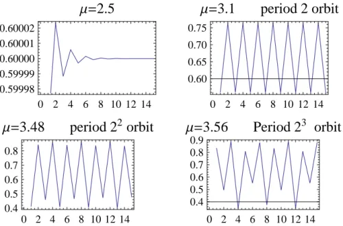
We can view this difference equation as the dynamical system xk+1=f(xk), wherefµ: [0,1]→[0,1]is defined by fµ(x) = µx(1−x). Although extremely simple in form, this one parameter family of dynamical systems exhibits a wide range of complicated dynamical behaviors (including chaotic behavior) and a rich bifurcation structure. This model was introduced into the population dynamics literature by May in [May, 2004]. While the mathematics of this family of models is rich, the applications to real populations are much less so, and it is difficult to find examples of populations which are well-modeled by logistic maps. For this reason I do not spend much time discussing this model.

The following facts can be found in many places, including [Weisstein, 2005].

1. The two fixed points arex= 0andx= (r−1)/r(forr >1).

2. If0≤µ <1, the fixed pointx= 0is globally attracting, i.e.,limk→∞xk= 0 for allx0.

3. If 1 ≤µ < 3, the fixed pointx = 0is unstable, and the fixed point x= (r−1)/r is attracting. Thus limk→∞xk= (r−1)/rfor0 < x0 <1. The map fµ has a transcritical bifurcation atµ= 1. See Figure 2.14.

4. If3≤µ <1+√6, there is an attracting period2orbit{x21, x22}such thatf(x21) =x22andf(x22) =x21. The

fixed pointsx= 0andx= (r−1)/rare both unstable. The limit limk→∞xk={x21, x22}for0< x0<1,

x06= 0,(r−1)/r. The mapfµ has a period doubling bifurcation atµ= 2. See Figure 2.14. 5. If µ2 = 1 +

√

6 = 3.449490· · · ≤ µ < µ3 = 3.544090. . ., there is an attracting period 22 orbit. All the

previous mentioned periodic points are unstable. The mapf2

µ has a period doubling bifurcation atµ2. See

Figure 2.14.

6. If µ3 = 3.544090· · · ≤ µ < µ4 = 3.564407. . ., there is an attracting period23 orbit. All the previous

mentioned periodic points are unstable. The mapf3

µ has a period doubling bifurcation atµ3. See Figure

2.14.

7. There is an infinite increasing sequence of parametersµk→µ∞= 3.5699456. . ., such thatf_µkhas a period

doubling bifurcation atµk which creates an attracting period2k orbit. All the previous mentioned periodic points of period{1,2,22_{, . . . ,}₂k−1_}_{are unstable. This infinite period doubling cascade is illustrated on the}

(31)

2.6. DISCRETE GROWTH MODELS 31

8. The map fµ∞ is usually called the Feigenbaum map. It has unstable period orbits of orders 2

n_{, n} ₌ 1,2,3, . . ., which together are dense in the unit interval. The map fµ∞ also has a non-chaotic strange

attractorΛ∞, which contains the closure of the unstable periodic points. This fractal set attracts the orbit

of almost every point in[0,1]. The restriction offµ∞ toΛ∞is minimal and topologically equivalent to an

adding machine. Thus it has zero topological entropy.

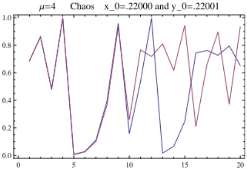
9. There is a saddle node bifurcation atµ= 3.829which creates a stable/unstable pair of period three orbits. These persist untilµ= 4. It follows from a result of Li and Yorke [Li and Yorke, 1975] that the associated mappingsfµ are chaotic, in the sense that they exhibit periodic points of all periods and uncountably many points with sensitive dependence on initial conditions. These maps have positive topological entropy.

10. The map f4 is smoothly conjugate to the tent map f(x) = 2x mod (1) on [0,1] via the conjugacy

h(x) = sin2(πx/2)and is semi-conjugate to the one-sided shift map on two symbols. Thusf4 is chaotic in

the strongest sense. See Figure 2.16.

An interesting question is whether there exist real populations which exhibit period doubling bifurcations or chaos. We will return to this question when we discuss modeling the population of flour beetles in Section 3.6.

2.6.2 Beverton-Holt model

Another way to discretize the logistic ODE is to find a difference equation that is the time-one map of the logistic ODE. This model was introduced by Beverton and Holt in their study of fisheries [Beverton and Holt, 1957] and can be written as

xn+1= Rxn

1 +xn/M

, (2.42)

whereR is the proliferation rate per generation andK= (R−1)M is the carrying capacity of the environment. It has the closed form solution

xn= Kx0

x0+ (K−n0)R−n

, (2.43)

which is precisely the time-n map of the logistic ODE (see Equation (2.13)). Thus the discrete Beverton-Holt modelf exhibits the same long term dynamics as the logistic ODE.

2.6.3 Ricker model

A third way to discretize the logistic ODE is to start with the modified ODE x=rx(t)(1−[x(t)]/k), where[x] denotes the greatest integer less than or equal tox. Integrating fromnton+ 1yields

x(n+ 1) =x(n) exp (r(1−x(n)/K)), (2.44)

for0≤n≤t < n+ 1. Lettingt→n+ 1, one obtains the Ricker difference equation

xn+1=xnexp (r(1−xn/K)). (2.45)

(32)

0 2 4 6 8 10 12 14 0.59998

0.59999 0.60000 0.60001 0.60002

Μ=

2.5

0 2 4 6 8 10 12 14 0.60

0.65 0.70 0.75

Μ=

3.1 period 2 orbit

0 2 4 6 8 10 12 14 0.4

0.5 0.6 0.7 0.8

Μ=

3.48 period 2

2

orbit

0 2 4 6 8 10 12 14 0.4

0.5 0.6 0.7 0.8 0.9

Μ=

3.56 Period 2

3

orbit

Figure 2.14: Periodic orbits of members of the quadratic family

(33)

2.7. STOCHASTICITY 33

0 5 10 15 20

0.0 0.2 0.4 0.6 0.8 1.0

Μ=4 Chaos x_0=.22000 and y_0=.22001

Figure 2.16: Chaotic behavior off4. Notice the sensitive dependence on initial conditions.

2.7 Natural catastrophes, genetic stochasticity, environmental

stochas-ticity, and demographic stochasticity

All populations exhibit random fluctuations. However, for small populations, these fluctuations are sometimes major determinants of population change and causes of extinction. The field of conservation ecology addresses population dynamics issues associated with the small population sizes of rare species, where the phenomena discussed in this section are crucial considerations.

Some investigators build stochasticity into their population models. They argue that adding stochasticity provides added flexibility to better fit real data, that invariant probability distributions of stochastic processes can provide additional insights, and that the simulation of stochastic models may be easier than for deterministic models.

Food shortages, disease, and extreme weather can all devastate populations. The following sad tale from [Shaffer, 1981] is illustrative.

(34)

2.7.1 Natural catastrophes

Natural catastrophes, such as floods, fires, droughts, or meteor strikes occur infrequently, and can cause the death of a large proportion of individuals. For the heath hens, the 1916 fire that destroyed most nests and habitat was an example of a natural catastrophe.

2.7.2 Genetic stochasticity

For small populations the amount of genetic material available for natural selection is small. Thus if conditions change, there may be less genetic variability for natural selection to act, which could result in extinction. For the heath hens, the sterility of the last survivors was an example of genetic stochasticity.

2.7.3 Environmental stochasticity

Environmental stochasticity is the variation in vital rates from one season to the next in response to weather, disease, predation, competition, or other factors external to the population. Environmental stochasticity can affect large populations, as well as small. For the heath hen, the excessive predation by goshawks in 1917 and disease in 1920 are examples of environmental stochasticity of survival rates.

The following is for students who have taken an advanced course in probability. A common way that authors incorporate environmental stochasticity is to add additive noise on the log scale. The simplest such extension of the exponential growth model is the stochastic ODE (SODE)

dNt=rNtdt+Ntdwt, (2.46) wherewtis a Wiener process, and the meaning of this expression is in the integral sense. I thank my Georgia Tech colleague Ionel Popescu for his patience in explaining to me the basic ideas behind analyzing SODEs. Integrating both sides one obtains

Nt=N0+

Z t

0

rNsds+ Z t

0

Nsdws, (2.47)

Taking expected values of both sides, and using the fact that the second integral is a martingale and the expected value of a martingale is zero, one obtains

E[Nt] =E[N0] +r

Z t

0

E[Ns]ds. (2.48)

This integral equation can be easily solved

E[Nt] =E[N0] exp (rt). (2.49)

Thus the expected value of the population size at time t coincides with the solution of the exponential growth model. To compute the population variance, we need to apply Ito’s formulam which is a funny looking version of the chain rule. It states that the processN2

t can be represented asdNt2= 2(r+ 1)Nt2dt+ 2Nt2dwt. Integrating both sides one obtains

dN2

t = Z t

0

2(r+ 1)N2

sds+ Z t

0

(35)

2.7. STOCHASTICITY 35

Taking expected values of both sides, one obtains

E[N2

t] =E[N02] + 2

Z t

0

(r+ 1)N2

sds. (2.51)

This integral equation can also be easily solved

E[Nt2] =E[N02] exp (2(r+ 1)t). (2.52)

It follows that the variance

V[Nt] = E[N2

t]−E[Nt]2 (2.53)

= E[N02] exp (2(r+ 1)t)−E[N0]2exp (2rt). (2.54)

Ast→ ∞, the coefficient of variationpV[N(t)]/E[N(t)]grows like q

E[N2

0] exp (t). (2.55)

Thus the population fluctuations become relatively greater as time gets larger and larger. The SODE (2.46) actually has a closed form solution. It follows from Ito’s formula that

Nt= exp ((r−1/2)t) exp (w(t)). (2.56) . This explicit formula allows easy computer simulations of the population process.

Problem 10. Consider the SODE modeling exponential population growth with random migration

dNt=rNtdt+dwt. (2.57)

Imitate the above calculations line by line to show that

E[Nt] = E[N0] exp (rt) and (2.58)

V[Nt] = V[N02] exp (2rt) + (exp (2rt−1))/r. (2.59)

2.7.4 Demographic stochasticity

Demographic stochasticity is the variability in vital rates arising from random differences among individuals in survival and reproduction within a season. Large populations are highly unlikely to experience significant variation of these averages. For example, if one assumes that a vital rate of individuals varies independently, then the variance is inversely proportional to the population size, and thus the fluctuations are negligible. However, for very small populations of100or fewer members, demographic stochasticity could cause extinction. For example, a long run of male births (think ten successive heads of a coin flip) could skew the sex ratio and substantially increase the risk of extinction by almost eliminating the number of breeding females.

An Mathematical Introduction to Population Dynamics