Anthropogenic carbon distributions in the Atlantic Ocean: data-based estimates from the Arctic to the Antarctic

www.biogeosciences.net/6/439/2009/

© Author(s) 2009. This work is distributed under the Creative Commons Attribution 3.0 License.

Biogeosciences

Anthropogenic carbon distributions in the Atlantic Ocean:

data-based estimates from the Arctic to the Antarctic

M. V´azquez-Rodr´ıguez1, F. Touratier2, C. Lo Monaco3, D. W. Waugh4, X. A. Padin1, R. G. J. Bellerby5,6, C. Goyet2, N. Metzl3, A. F. R´ıos1, and F. F. P´erez1

1_{Instituto de Investigaciones Marinas, CSIC, Eduardo Cabello 6, 36208 Vigo, Spain} 2_{IMAGES, Universit´e de Perpignan, 52 avenue Paul Alduy, 66860 Perpignan, France} 3_{LOCEAN/IPSL, Universit´e Pierre et Marie Curie, case 100, 75252 Paris cedex 05, France} 4_{Department of Earth and Planetary Sciences, Johns Hopkins University, Baltimore, USA}

5_{Bjerknes Centre for Climate Research, University of Bergen, All´egaten 55, 5007 Bergen, Norway} 6_{Geophysical Institute, University of Bergen, All´egaten 70, 5007 Bergen, Norway}

Received: 4 March 2008 – Published in Biogeosciences Discuss.: 7 April 2008 Revised: 21 January 2009 – Accepted: 9 March 2009 – Published: 18 March 2009

Abstract. Five of the most recent observational methods to estimate anthropogenic CO2(Cant) are applied to a high-quality dataset from five representative sections of the At-lantic Ocean extending from the Arctic to the Antarctic. Be-tween latitudes 60◦_N–40◦_{S all methods give similar spatial} distributions and magnitude of Cant. However, discrepan-cies are found in some regions, in particular in the South-ern Ocean and Nordic Seas. The differences in the SouthSouth-ern Ocean have a significant impact on the anthropogenic carbon inventories. The calculated total inventories of Cantfor the Atlantic referred to 1994 vary from 48 to 67 Pg (1015g) of carbon, with an average of 54±8 Pg C, which is higher than previous estimates. These results, both the detailed Cant dis-tributions and extrapolated inventories, will help to evaluate biogeochemical ocean models and coupled climate-carbon models.

1 Introduction

Understanding and modelling the marine carbon system is one of the pressing issues within the framework of climate change. Carbon dioxide, an important greenhouse gas, is being increasingly produced by human activities, adding to the “natural” carbon cycle. International research has made progressive efforts to monitor the evolution of the oceanic sink of atmospheric CO2, and in understanding how human

Correspondence to:

M. V´azquez-Rodr´ıguez (mvazquez@iim.csic.es)

activities interfere with this air-sea coupled system. One of the grand aims of this effort is to accurately assess the future possible scenarios proposed by the Intergovernmental Panel on Climate Change (IPCC Fourth Assessment Report: Cli-mate Change 20071). The invasion of anthropogenic CO2 (Cant)in the ocean impacts not only the atmospheric carbon dioxide concentrations and is associated to climate change, but has also a direct effect on ocean chemistry, causing the so-called “ocean acidification” (Feely et al., 2004). The largest ocean acidification influences for the environment are expected to occur in the high northern and southern latitudes (Bellerby et al., 2005; Orr et al., 2005).

In this context, estimating Cant concentrations in the oceans represents an important step towards a better evalua-tion of the global carbon budget and its rates of change. Since Cantmay not be directly measured in the ocean it has to be derived from in-situ observations, under several assumptions. The pioneering original works by Brewer (1978) and Chen and Millero (1979) addressed this issue, and estimated Cant in Atlantic subsurface water masses of the Atlantic Ocean from total inorganic carbon (CT)measurements. They cor-rected the measured CTfor the effect of organic matter rem-ineralization (ROM) and made an estimate of the preformed Preindustrial CT(CTwhen the water was last in contact with the 1850 atmosphere). Together with the ROM contribution this preindustrial CT was also subtracted from the observed CT. In the last ten years, several observational (data-based) methods have been investigated at regional and global scales (see Wallace et al., 2001 for a historical overview). Two of

them, the1C∗ _{method (Gruber et al., 1996) and the} Tran-sient Time Distribution (TTD) method (Hall et al., 2002) have been applied at global scale. By using the 1C∗ ap-proach, Sabine et al. (2004) estimated a global oceanic in-ventory of Cantfor a nominal year of 1994 of 118±19 Pg C, which represents about 45% of the fossil fuel CO2emitted between 1800 and 1994. Similarly, Waugh et al. (2006) ap-plied the TTD method to estimate the Cantinventory for the global ocean and obtained results ranging between 94 and 121 Pg C for 1994. These authors also compared the Cant distribution derived from the1C∗and TTD approaches and pointed out that in spite of the grand-scale reasonable agree-ment, substantial differences occurred in the North Atlantic, South-Eastern Atlantic and in all basins south of 30◦S. This was an important result as it offered a range of Cant concen-trations to be used as a benchmark to be checked with ocean carbon cycle models. Analogous results were derived from intercomparison studies carried out with Ocean General Cir-culation Models (OGCM) (Orr et al., 2001), i.e.: reasonable agreement was found for ocean-wide inventories but signif-icant differences prevailed at a regional scale in terms of in-ventory and as to where Cantwas actually located, especially in the high latitudes and between the upper and lower ocean. Estimating accurate oceanic Cant inventories does not only provide a good constraint for predictive ocean models. They are also key input parameters in inverse models for calcu-lating air-sea fluxes of Cant (Gloor et al., 2003; Mikaloff-Fletcher et al., 2006; Gerber et al., 2009) and global budgets of the carbon cycle (IPCC, 2007).

In more recent years, additional data-based methods were developed in an attempt to improve the existing oceanic Cant estimates, especially at a regional level. These are the TrOCA method (Touratier and Goyet, 2004; Touratier et al., 2007), the C◦_IPSL method (Lo Monaco et al., 2005a) and theϕC◦_T method. To date, only few of these observa-tional methods, including the 1C∗, have been objectively inter-compared, and that is at regional scales only, namely: in the North Atlantic (Wanninkhof et al., 1999; Friis et al., 2006; Tanhua et al., 2007), the North Indian (Coatanoan et al., 2001), or along a single section in the Southern Ocean (Lo Monaco et al., 2005b). All of these studies identified significant discrepancies in Cantdistributions and specific in-ventories depending on the location, set of compared Cant estimation approaches and methodological assumptions.

Today, there is a pressing need to compare and clarify the Cantestimates from these various observational methods, as it has been analogously addressed in the case of ocean car-bon models (OCMIP project; Orr et al., 2001), atmospheric inverse models (Gurney et al., 2004), or coupled climate-carbon models (C4MIP project2).

2_{http://www.atmos.berkeley.edu/c4mip/}

As a contribution to the European integrated project of CARBOOCEAN, this international collaborative study will focus on the comparison of results from five different ap-proaches used to estimate anthropogenic CO2 concentra-tions. This is done from a single and common high-quality data set from modern cruises conducted in the Atlantic Ocean, including the Arctic and Southern Ocean sectors. The results will identify the areas of greatest discrepancies and uncertainty amongst methods. Based on the fundamentals and main assumptions of the methods some adjustments will be proposed to try to improve the estimates and reconcile methods upon. In addition, the results will also serve obser-vational and numerical ocean modellers to evaluate their sim-ulations and will help to reach a consensus as to where Cant is captured and actually stored. The analysis in the present work investigates the high latitudes (Southern Ocean and Nordic Seas) as locations where uncertainties are expected to be large for both data-based methods (Lo Monaco et al., 2005b; Waugh et al., 2006) and OGCMs (Orr et al., 2001). The Atlantic Ocean has been selected here because it has the largest Cantspecific inventory of all ocean basins, and also because of its large meridional and zonal gradients of Cant (Sabine et al., 2004; Waugh et al., 2006). The paper first de-scribes the various Cant meridional and zonal distributions, according to the different methods applied, focusing on key areas (of water masses formation and transformation). The specific and total Cantinventories are then presented and dis-cussed on the basis of the main assumptions from the meth-ods as possible sources for the observed dissimilarities.

2 Method

Data from four selected meridional sections (NSeas-Knorr, CLIVAR A16N, WOCE I06-Sb and WOCE A14) cover the length of the Atlantic and give a representative coverage of it (Fig. 1a). The WOCE AR01 extends from the Atlantic east to west ends at∼24◦N (Fig. 2a). They have all been re-cently conducted within the framework of either the WOCE or CLIVAR programs, except for the cruise in the Nordic Seas (NSeas, 2005) on board the R/V Knorr (Bellerby et al., 2005; Olsen et al., 2006). The data are available from the GLODAP website3, except for the NSeas data4 and the CLIVAR repeat section A16N legs 1 and 2 conducted dur-ing 20035. The selected cruises correspond to different years and thus Cantresults had to be referred to the common year 1994 (GLODAP canonical year) to eliminate biases intro-duced by the effect of increasing fugacity of atmospheric CO2 (fCO2). This was done using data from time series of CO2 molar fractions (xCO2)and calculating from here the ratio of Cantsaturation concentrations for the year of the

3_{http://cdiac.ornl.gov/oceans/glodap/Glodap home.htm} 4_{http://cdiac.ornl.gov/ftp/oceans/CARINA/Knorr/}

316N20020530/

c)

Age from CFC-12 (years)

Salinity

C_ant TTD (µmol·kg-1₎ C_ant TrOCA

(µmol·kg-1₎

C_ant Cº_IPSL (µmol·kg-1₎ C_ant ϕC_Tº

(µmol·kg-1₎

Cant ΔC*

(µmol·kg-1₎

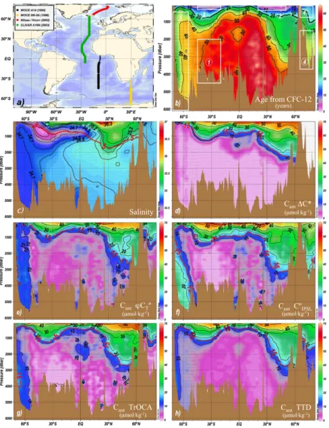
Fig. 1. (a)Map showing the considered meridional cruises WOCE A14, WOCE I06-Sb, CLIVAR A16N and NSeas/Knorr conducted in the

Atlantic. Thinner dots in cruises A14 and I06-Sb represent stations not used (latitudinal overlapping of different cruises);(b)age (years) of water masses in the meridional transects from (a), calculated using CFC12. The inlayed rectangles delimit the regions where Cantestimates

are given a closer look, namely: 1=deep South Atlantic, 2=northern and southern subtropical gyres, 3=Southern Ocean and 4=The Nordic Seas;(c)salinity distribution of the meridional transect displaying the 5◦C isotherm that separates the large volume of cold waters (_∼86% of the Atlantic Ocean volume) from warmer surface waters; (d–h) estimates of anthropogenic CO2(µmol kg−1)in the meridional transect

from the1C∗,ϕC◦_T, C◦_IPSL, TrOCA and TTD methods, respectively. The red 15µmol kg−1isopleth separates the region of maximum Cant

gradient from deeper waters.

cruise and the preindustrial era. The correction typically var-ied between 1–7µmol kg−1of Cantdepending on the pling year, the potential temperature and salinity of the sam-ples. Another consideration has been the overlapping lati-tudes of the A16N-A14 and A14-I06Sb section pairs. The general selection criteria followed was choosing the stations that were deepest and had the least influence of Indian Ocean waters. Accordingly, the northernmost ends of the A14 and I06Sb cruises are omitted from the plots (Fig. 1a). Finally, negative Cantestimates that were within the specific range of

uncertainty in each method were set to zero (ad hoc), while values more negative than that were taken as outliers and ex-cluded from subsequent analysis.

Salinity

C_ant TTD (µmol·kg-1₎ C_ant TrOCA

(µmol·kg-1₎

C_ant Cº_IPSL (µmol·kg-1₎ Cant ϕCTº

(µmol·kg-1₎

Cant ΔC*

(µmol·kg-1₎ Age from CFC-12

(years)

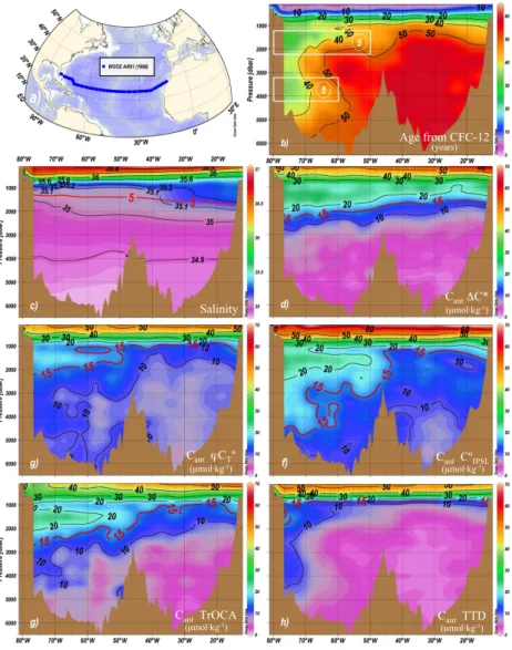
Fig. 2.Analogous contour plots to Fig. 1 for the zonal cruise WOCE AR01. From top to bottom and left to right:(a)cruise map,(b)CFC12

age in years showing theuDWBC andlDWBC limbs in white-contoured boxes numbered as “5”;(c)salinity field with the red 5◦C isotherm overlaid; (d–h) Cantconcentration estimates (µmol kg−1)from the1C∗,ϕC◦_T, C◦_IPSL, TrOCA and TTD methods, respectively.

from the Cantappearing in the GLODAP dataset as of Lee et al. (2003). They have applied the1C∗method to evaluate the inventory of Cantin the eastern and western basins of the At-lantic. Their Cantestimates have been included in the global synthesis of Sabine et al. (2004) and the GLODAP database (Key et al., 2004). The data used and Cant results obtained using the above methods are available under the Carboocean data portal to facilitate further comparisons with OGCM out-puts, for instance, that are beyond the scope of the present work. The above methods can be classified into two groups on the basis of the variables needed to compute Cant: a) the Transient-Tracer-based methods (TTD) that commonly use CFC11 or CFC12 concentration measurements as proxies of the anthropogenic CO2signal and b) the Carbon-based meth-ods (1C∗, C◦_IPSL,ϕC◦_T and TrOCA) which typically require

measurements of dissolved inorganic carbon (CT), total al-kalinity (AT), oxygen, temperature and eventually salinity and some nutrient analysis. They all make a steady-state as-sumption in terms of seasonal and interannual variability of the natural carbon cycle.

CO2 disequilibrium is considered to be constant over time, but not in space. The use ofpCFC12 age to calculate the date of formation of the water masses is a potential positive bias in the method. This is because the CFC12 history is shorter and more nonlinear than surface Cant, and using the CFC12 age as the single ventilation means one looks too recently in the surface Cant history and overestimates Cant (Hall et al., 2002). This bias tends to increase withpCFC12 age, and is expected to be large for deep waters withpCFC12 ages greater than 25 years (Matear et al., 2003).

The classical 1C∗ approach is fundamentally based on the preformed CTback-calculation principles established by Brewer (1978) and Chen and Millero (1979). To constitute a measure of Cantin a water sample the method back-calculates the CTof a water sample to its initial (preformed) CT concen-tration when it was last at surface on the basis of the changes in AT, AOU, salinity and θ. The1C∗ _{approach is} princi-pally based on two assumptions: a) the anthropogenic CO2 invasion has not altered surface alkalinity, so that it is un-necessary to differentiate between historical and present pre-formed alkalinity (A◦_T)values and b) constant air-sea CO2 disequilibrium (1Cdis)over time at the source region of the sampled water (steady state assumption). The method first introduced the1Cdisterm to the back-calculation techniques and proposed a formal way to estimate it. In old water masses, according to apCFC11 age criteria, Cantwas auto-matically set to zero and1Cdiswas assigned the value of the quasi-conservative tracer1C∗. For younger water masses, the1Cdis had to be estimated using the “shortcut” method (Thomas and Ittekot, 2001) to calculate Cantdirectly on those waters, based on their CFC11 content. One caveat to this pro-cedure is that it can misleadingly prone to think that all wa-ters void of CFCs are unaffected by Cant(Matear et al., 2003). Knowingly, this conjecture introduces negative biases on the

1C∗ (Matsumoto and Gruber, 2005). It must alternatively be noticed that the1C∗approach considers that waters are fully saturated with oxygen and CFCs at the instant of their outcropping.

The C◦_IPSL method is based on the original C◦ method described in the works by Brewer (1978) and Chen and Millero (1979). Differently, it allows for air-sea oxygen dis-equilibria. In most regions of the world ocean (including the North Atlantic) the preformed oxygen is close to equi-librium with the atmosphere. In the Southern Ocean, the up-welling of oxygen-exhausted waters provokes a deficit in sur-face oxygen concentrations of up to 50µmol kg−1_(Poisson and Chen, 1987). A mean oxygen under-saturation coeffi-cientα=12% calculated in the Weddell Sea area (Anderson et al., 1991) was used for Cantcalculation in ice-covered sur-face waters. This method uses different preformed relation-ships of A◦_Tand C◦_Tfor southern and northern Atlantic waters. The relationships for the Southern Hemisphere were deter-mined from winter data collected in surface waters (0–50 m) in the Atlantic and Indian Oceans. Northern relationships were determined using subsurface measurements (50–150 m)

collected in the North Atlantic and Nordic Seas. The specific contributions of northern and southern waters are introduced in the equations via a specific north-south mixing ratio “k”. The coefficients for each sample are determined with a multi-ple end-member mixing model they resolved via an optimum multiparameter (OMP) analysis. The RC andRN stoichio-metric ratios used are the ones determined by Anderson and Sarmiento (1994). The preindustrial Cantreference is calcu-lated from North Atlantic Deep Water (NADW) detected in the South Atlantic, where Cantconcentrations are below de-tection limits. This zero-Cantbaseline reference corresponds to the increase in C◦_Tin the source region since the preindus-trial era, and although it is a time-dependent parameter it is applied as a constant (−51µmol kg−1).

TheϕC◦

Tmethod is another process-oriented biogeochem-ical approach to estimate Cant in the Atlantic that follows the same fundamental principles as the1C∗_{or C}◦

IPSL back-calculation methods. The subsurface layer (100–200 m) is taken in theϕC◦_Tmethod as a reference for characterising wa-ter mass properties at the moment of their formation. The air-sea disequilibrium (1Cdis)is parameterized at the subsurface layer first using a shortcut method to estimate Cant. Since the average age of the water masses in the 100–200 m depth do-main, and most importantly in outcropping regions, is under 25 years, the use of the shortcut method to estimate Cantis ap-propriate (Matear et al., 2003). The A◦_Tand1Cdis parameter-izations (in terms of conservative tracers) obtained from sub-surface data are applied directly to calculate Cantin the water column for waters above the 5◦C isotherm and via an OMP analysis for waters with θ <5◦_{C. This approach especially} improves the estimates in cold deep waters that are subject to strong and complex mixing processes between Arctic and Antarctic water masses and represent an enormous volume of the global ocean (∼86%). One important aspect in this process is that none of the A◦_Tor1Cdisparameterizations are CFC-reliant. The ϕC◦_T method proposes an approximation to the horizontal (spatial) and vertical (temporal) variability of 1Cdis (11Cdis)in the Atlantic Ocean in terms of Cant and1Cdis itself. Also, the small increase of A◦_T since the Industrial era due to CaCO3 dissolution changes projected from models (Heinze, 2004) and the effect of rising sea sur-face temperatures on the parameterized A◦_Tare accounted for. These two last corrections are minor but should still be con-sidered if a maximum 4µmol kg−1bias (2µmol kg−1on av-erage) in Cantestimates wants to be avoided.

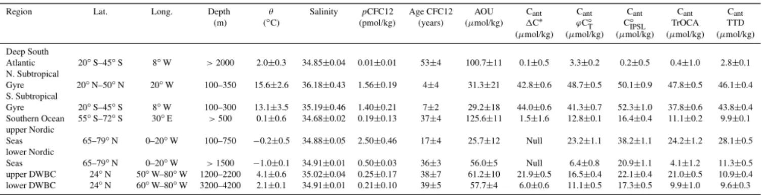
Table 1.Summary statistics for the regions highlighted in Figs. 1b and 2b.

Region Lat. Long. Depth θ Salinity pCFC12 Age CFC12 AOU Cant Cant Cant Cant Cant

(m) (◦C) (pmol/kg) (years) (µmol/kg) 1C∗ ϕC◦_T C◦_IPSL TrOCA TTD (µmol/kg) (µmol/kg) (µmol/kg) (µmol/kg) (µmol/kg) Deep South

Atlantic 20◦S–45◦S 8◦W >2000 2.0±0.3 34.85±0.04 0.01±0.01 53±4 100.7±11 0.1±0.5 3.3±0.2 0.2±0.5 0.4±1.0 2.8±0.1 N. Subtropical

Gyre 20◦N–50◦N 20◦W 100–350 15.6±2.6 36.18±0.43 1.56±0.19 4±4 31.3±21 42.8±0.6 48.7±0.5 50.1±0.9 47.8±0.5 46.1±0.4 S. Subtropical

Gyre 20◦S–45◦S 8◦W 100–300 13.1±3.5 35.19±0.46 1.40±0.21 7±2 29.2±18 44.0±0.6 41.3±0.7 52.3±1.0 37.8±0.6 43.8±0.4 Southern Ocean 55◦S–72◦S 30◦E >500 0.1±0.6 34.68±0.02 0.19±0.13 37±4 125.6±11 1.5±1.6 12.8±0.1 16.4±0.4 11.1±0.2 9.9±0.1 upper Nordic

Seas 65–79◦N 0–20◦W 100–750 −0.2±0.5 34.88±0.05 2.50±0.46 17±4 25.7±12 Null 23.2±1.1 38.2±1.1 24.2±1.2 28.1±0.5 lower Nordic

Seas 65–79◦N 0–20◦W >1500 −1.0±0.1 34.91±0.01 0.50±0.03 36±3 56.0±5 Null 6.4±0.8 20.9±1.1 4.1±1.2 11.3±0.5 upper DWBC 24◦N 50◦W–80◦W 1200–2200 4.1±0.6 35.02±0.04 0.25±0.17 38±7 61.2±10 21.9±0.5 16.5±0.4 22.1±0.4 21.0±0.5 10.9±0.4 lower DWBC 24◦N 60◦W–80◦W 3200–4200 2.1±0.1 34.91±0.01 0.21±0.10 39±5 57.7±4 6.0±0.6 11.1±0.5 17.3±0.5 9.9±1.0 9.6±0.3

the increase of atmospheric CO2 (Chen and Millero, 1979; Goyet et al., 1999), i.e. A◦

T=AT; and that O◦2≈O2. The equa-tion for the reference term TrOCA◦ _{is a function ofθ and} AT. This equation is derived from 114C and correspond-ing to water parcels that can be assumed to be free of Cant. When the concentration of114C<175 per mille, the approx-imate age of the corresponding water mass is greater than 1400 years, long before the beginning of human CO2 mas-sive emissions. The samples with maximum CFC11 concen-trations, typically between 262.9 and 271.3 pptv correspond-ing to surface waters in 1992–1995 (maximum atmospheric

pCFC11), were also selected as part of the dataset to obtain the TrOCA◦expression.

3 Results and discussion

3.1 Anthropogenic CO2distributions

The meridional distributions of Cant calculated from the

1C∗_{, ϕC}◦

T, C◦IPSL, TrOCA and TTD methods are shown in Fig. 1d–h, respectively. The spatial patterns are sim-ilar in all calculations. The maximum Cant values (40– 60µmol kg−1)are consistently located in the northern sub-tropical gyre (20◦N, 50◦N), where the intensification of the Meridional Overturning Circulation (MOC) also provokes the strongest water mass outcrops and deepest Cant trans-port. Alternatively, Cantminima are unanimously located un-der the southern subtropical gyre below 1500 m, where the oldest water masses are found in the Atlantic eastern basin (Fig. 1b). There is also general agreement in the area of largest Cantgradients, just above the 15µmol kg−1isopleth. The strong water mass formation processes in the North At-lantic subpolar gyre (Schmitz, 1996) have a large effect on the dynamics of Cantoceanic uptake. They provoke the dif-ferent Cantdistributions observed in the Nordic Seas, where the 15µmol kg−1_{isoline shallows abruptly.}

The results for the WOCE AR01 cruise (Fig. 2) show a similar degree of agreement to the meridional section just

described. There are three distinctive features to the AR01 section: a) the upper 1000 m are characterised by a strong vertical Cantgradient, from 60 to 20µmol kg−1_{; b) the} min-imum values (0–15µmol kg−1_{)are consistently located in} the eastern Atlantic Basin; c) the entrainment eastwards of the Deep Western Boundary Current (DWBC) upper limb is detected unanimously around 1500 m, whereas its lower limb (3000–4000 m) is not always as clearly seen in the Cantfields. In spite of the similarities in the large-scale Cant distri-butions, there are some significant variations at a regional scale, most notably in the Antarctic Bottom Water (AABW) and the Nordic Seas. Below we discuss in more detail the distributions in several different regions, shown as boxes in Figs. 1b and 2b (see also Table 1). For each region, the av-erage values of several quantities are listed in Table 1, and the average Cantconcentration is plotted againstpCFC12 in Fig. 3. Whenever two or more results from different meth-ods are compared within a region, a hypothesis contrast is applied with confidence levelα=0.05, considering the num-ber of data (N) and using the population means of the stan-dard errors of the mean (σ/√N). Vertical profiles of average Cantconcentrations for the latitudes or longitudes covered by the above regions are also shown in Fig. 4 (note that several of these profiles include two of the boxed regions shown in Figs. 1b and 2b).

Fig. 3. Average regional Cant estimates (µmol kg−1) predicted

by the five Cantreconstruction methods here considered plotted in

increasing order of averagepCFC12 (patm) concentration on the

studied regions. Notice that thepCFC12 scale is nominal and there-fore non-linear. The error bars give the standard error of the mean (_±σ/√N).

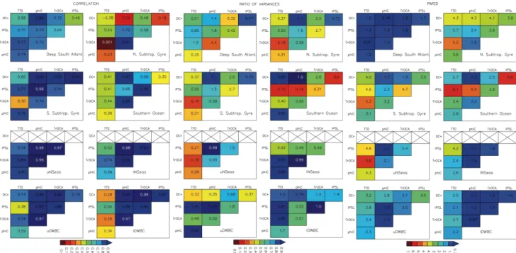
very well (i.e. low RMSD andR, andγ near unity) as well as other ones where there are large differences. These differ-ences are discussed in more detail below, but in general, com-parisons of the TTD estimates with the other estimates yield the largest differences, i.e., the highest RMSDs, lowestR, and values ofγ furthest from unity. TheϕC◦_Tmethod gener-ally shows the opposite: it genergener-ally has the lowest RMSDs, highestR, andγ values closest to unity. Interestingly, but perhaps not surprising, the carbon-based methods TrOCA, C◦_IPSLandϕC◦_Tcome out highly correlated independently of the region considered.

3.1.1 Deep South Atlantic

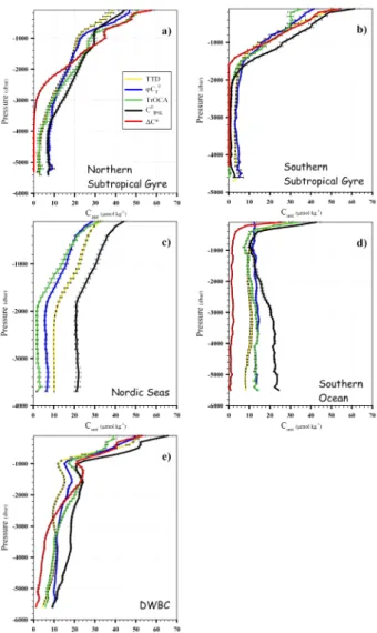
The oldest water masses in the Atlantic are found in deep waters around 30◦_{S and they are expected to have near-zero} Cant loads (Figs. 1b, 3 and Table 1). Deeper than 2000 m the average Cantvertical profiles from all methods stabilize at very low values, however the actual values differ between methods, with 1C∗, and C◦_IPSL estimates being the lowest and TTD and ϕC◦_T the largest (Fig. 4b). Most 1C∗ esti-mates for this region were either missing values or outliers and, therefore, excluded from inventory computations. In addition, the1C∗ method defines its absolute zero-Cant at the deep, very old waters based on CFC or114C age esti-mates. Analogous comments apply to the results from the C◦_IPSLmethod, although this method does not report as many negative or missing values as in the1C∗case. The RMSD values in this region are low for all pairs of methods, which is likely related to the low average Cantconcentrations in the very old waters. The correlation between methods is general high, with the highestRfor1C∗_-ϕC◦

Tcorrelation (Fig. 5).

Fig. 4. Average vertical Cantprofiles (µmol kg−1)of the selected

regions in Figs. 1b and 2b. The Cantestimates in each region were

averaged over common depth intervals and the error bars represent the standard error of the mean (±σ/√N).

3.1.2 Subtropical gyres

The northern subtropical gyre, with an observed average age of 4 years (right-hand Box 2 in Fig. 1b), contains on average the highest Cantconcentrations andpCFC12 values (Fig. 3). The carbon-based methods TrOCA, C◦

Fig. 5.Array of statistics for each of the regions highlighted in Figs. 1b and 2b. The Pearson’s product-moment correlation coefficient (R), Root Mean Square Difference (RMSD, inµmol kg−1)and ratio of variances (γ) were calculated for all method pairs. In all cases the more bluish the colour the better the agreement (dark blue forR=_±1, RMSD=0, andγ=1). For the ratio of variances,γ and 1/γ are the same

colour. Here, RMSD=

s

1/N

N

P

i=1

Ai−A

− Bi−B

2

, where Aiis thei-th Cantestimate of the considered method “A” in the comparison

pair, and “A” is the average of the subset of estimates considered from method “A”. The terms Biand “B” are analogously defined for method

“B”. N stands for the number of valid A-B data pairs.

TTD value by 3.3µmol kg−1(Fig. 3 and Table 1). The Cant estimates in the southern subtropical gyre are similar to the northern counterpart, but with slightly lower average Cant concentrations and less Cant entrainment into the ocean in-terior (Fig. 4b and c). The above-described differences trans-late into different vertical Cantgradients. In the southern sub-tropical gyre the C◦

IPSLand1C∗have stronger vertical Cant gradients than the rest of methods (Fig. 4b). This same pat-tern is observed in the northern subtropical gyre but it does not appear to be so clear due to the larger penetrations of Cant in the water column (Fig. 4c). Lastly, it is worth noting from Figs. 1d–h and 4c that all methods detect the Mediterranean water (MW) influence, which causes a relative maximum of Cant(average 22.6±3.5µmol kg−1)at about 1100 m depth at 37◦N (R´ıos et al., 2001; ´Alvarez et al., 2005; A¨ıt-Ameur and Goyet, 2006). Large RMSDs are found for both subtropi-cal gyres, and there is also a generalised tendency towards low correlation values. The most extreme values occur in the northern gyre, where there are generally very large RMSD and very low correlations between TTD and1C∗ and the other methods, and between TTD and1C∗_{. In fact, out of} all the studied regions and method pairs considered, the case of the TTD and1C∗_{in the northern subtropical gyre is the} only where two methods have yielded Cantestimates that are inversely correlated.

3.1.3 The Nordic Seas

as 5.9µmol kg−1_{(TTD-TrOCA). This gives an idea of how} variable the average vertical Cantprofiles are with respect to the TTD, especially in the upper Nordic Seas. Nevertheless, the TTD vertical profile (Fig. 4c) represents quite the average of all methods in this region, most importantly in the lower Nordic Seas, and this is somewhat reflected by the associ-atedR andγ values. The lowest γ for this region corre-spond to all method pairs involving the TTD (γ_∼0.22) and IPSL (γ_∼0.47) methods in the upper and lower Nordic Seas, respectively.

3.1.4 The Southern Ocean

South of 50◦S the different methods, although applied to the same dataset, present very contrasting results. The average Cantvertical profiles (Fig. 4d) share similar patterns: moder-ate values in the first 500 m before they suddenly drop into a plateau of almost constant concentrations in the rest of the water column. This trend is slightly different for C◦_IPSL and

ϕC◦_T. For the former there is a tendency of Cantto increase with depths below 1000 m, while the latter has a very sta-ble vertical profile centred at∼12.5µmol kg−1. The AABW forms in this region from Circumpolar Deep Water (CDW) and Ice Shelf Waters (ISW), potentially driving in the South-ern Ocean an intense conveyance of Cantdown to the seafloor (>5000 m). The fact that Cantmay have penetrated this far down in the Southern Ocean is also suggested by the pres-ence of CFC12 in the water column (Box 3 in Fig. 1b and Fig. 3). Consequently, the TTD method (based mainly on CFC12 data) produced Cantdown to the bottom at high lat-itudes, a signal that was not captured in the 1C∗ _results (Figs. 3 and 4d) (Lo Monaco et al., 2005a, b; Waugh et al., 2006). Interestingly, the other methods (TrOCA, C◦_IPSL and

ϕC◦_T)also detected significant Cantconcentrations in the deep and bottom waters of the Southern Ocean. The TTD,ϕC◦_T and TrOCA methods have very similar vertical Cantprofiles below 1000 m (Fig. 4d). The1C∗predictions give close-to-zero Cantvalues (1.5±1.6µmol kg−1)and are clearly lower than other estimates. The 1C∗ method assigns by default Cant=0 references to old waters with low CFC concentra-tions, like those found below 500 m depths in the neighbour-ing regions of the South Atlantic (Gruber et al., 1996). Also, the1C∗approach assumes oxygen saturation in surface wa-ters. The low results obtained in this area could follow from this assumption (Lo Monaco et al., 2005a). Nevertheless, it must be noted that authors like Sabine et al. (2002), by applying the1C∗ _{method in other sectors of the Southern} Ocean, have obtained higher Cantestimates. The fact that the Southern Ocean is a large volume of water means that small differences between methods will ultimately translate in sig-nificant inventory differences in this region (Lo Monaco et al., 2005b). In terms of statistics, the largest RMSD values of all regions are found in this region, and there are also low correlation coefficients andγ far from unity, indicating how disparate are the Cantestimates in this region.

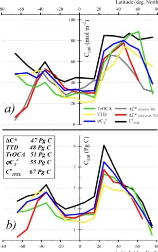
Fig. 6. Specific inventories(a)in mol m−2for the whole Atlantic

computed in latitude bands every 10◦, after Lee et al., 2003. The total inventories (Pg C) for the same domain and latitude band res-olution are plotted in(b). The inlayed box gives the integrals of the presented total inventories (Pg C) for each method in the Atlantic Ocean.

3.1.5 The Deep Western Boundary Current (DWBC) The DWBC is detected in Cant from all methods (Fig. 2b). However, there are differences in the intensity of the vertical Cant gradient generated by the upper limb (uDWBC), cen-tred around 1500 m, and the lower limb (lDWBC), centred around 3500 m. The clearest signal in the DWBC is given by the C◦

deeper than in the rest of methods. Finally, it is also notable that the eastward deflection and propagation of the North At-lantic Deep Water upper limb (uNADW) coming from the

uDWBC (Weiss et al., 1985; Andri´e et al., 1998) can also be observed in Fig. 1: a Cantmaximum located at 1500–2000 m depth in the Equator corresponding with a relative minimum of CFC12 age (∼50 yr) is detected to different extents by all methods. There are low RMSDs between most pairs of methods for both limbs. The methods are generally highly correlated and have similar variances. The TTD method is the exception with regard to the correlations, and there are low correlations between the TTD and other methods in the

lDWBC.

3.2 Atlantic inventories of anthropogenic CO2

To assess how the previous differences in the various data-based Cantestimates affect the global Cantbudget, the results were integrated on the Atlantic basin scale. In calculating the inventory the following considerations were made: a) the wa-ter column integrals were calculated over the same 10-degree wide latitude bands as in Lee et al. (2003). In so doing, the results obtained can be compared with their estimates from the1C∗ method; b) no in situ surface Cant estimates were used at all so as to avoid the seasonal biogeochemical vari-ability from surface layer data. Instead, values from the bot-tom limit of the winter mixed-layer were extended to 0 m, so that Cant from surface waters is still being considered in inventory calculations (Lo Monaco et al., 2005b). On the basis of winter mixed layer depths the location of the bot-tom limits were placed at 100 m in subtropical and equatorial waters, and at 300 m for waters in the (33◦_S–50◦_{S) latitude} band; c) regarding total inventories, the meridional cruises used in this study belong to the eastern Atlantic basin. To tackle the zonal asymmetry assumption, results in Table 5 from Lee et al., 2003 were used. They provided specific in-ventories (mol m−2)for the eastern and western basins and the total inventories (Pg C) for different latitude bands. A conversion factor per band of latitude (1.04±0.10) that ac-counted for the area was calculated using the eastern basin specific inventory and the total inventory data from Lee et al., 2003. Given the similarities here found in the general Cantdistributions it is assumed that the scaling obtained for the1C∗from Lee et al. (2003) can be applied to the rest of methods. Knowingly of the caveats attached to this practice, this assumption allows to calculate Atlantic inventories from the presented eastern Atlantic basin results; d) the Cant inven-tories from Gruber (1998) and Lee et al. (2003) are included in Fig. 6a to show how the1C∗method yields very low val-ues in the Southern Ocean, regardless of the dataset to which it is applied (Lo Monaco et al., 2005a). These inventories were calculated from different data collected over the same region here studied, and were referenced to year 1994; e) The errors for the specific inventories are of±1 mol m−2or

±2 mol m−2when integrated down to 3000 m or 6000 m,

re-spectively. They were calculated by means of random prop-agation of a 5µmol kg−1_{standard error of the Cant estimate} with depth. Error bars in Fig. 6a are omitted for clarity.

All methods give reasonably similar specific inventories (Fig. 6a), except for the1C∗method in the Southern Ocean from either Gruber (1998) or Lee et al. (2003). The greatest similarities occur in the subtropical and equatorial regions, while some discrepancies between the C◦_IPSL,ϕC◦_T, TrOCA and TTD methods appear towards higher latitudes, especially north from 55◦_{N, where none of the estimates converge. In} the Southern Ocean (south of 55◦_{S), the1C}∗_{method shows} extremely low values (10_±5 mol m−2_{on average)} consider-ing the non-negligible amount of CFCs found in this basin (Fig. 1b). These estimates are five to seven times lower than any other result in this area. The strong decreasing trend of the specific inventories according to the1C∗approach is also opposite to the other carbon-based methods which de-scribe increasing specific inventories south from 45◦S. More substantial differences were identified in other regions: in the Tropics, the TTD method gives about half the amount of Cant the C◦_IPSLmethod does, and in the North Atlantic differences of 20 mol m−2are common.

The specific inventories were integrated by area to calcu-late the total inventories (in Pg C) over the same bands of latitude (Fig. 6b). In so doing, the aforementioned differ-ences in the Nordic Seas diminish. All methods display an “M-shape” in the total inventory distribution, with a coher-ent maximum around 20–30◦N and a relative maximum at 40–50◦S. Although significant differences can still be seen between methods, we believe that the “M-shape” describes faithfully oceanic anthropogenic CO2 fields and should be reproduced by ocean and climate models. The total invento-ries for the Atlantic basin (excluding the Nordic Seas), re-ferred to 1994 estimated by the C◦

IPSL, ϕC◦T, TrOCA and TTD methods are: 67, 55, 51 and 48 Pg C, respectively (av-erage 55_±8 Pg C; Fig. 6b). These results are higher than the 47 Pg C inventory given by Lee et al. (2003) using the1C∗ approach, and if this1C∗estimate is to be included then the average Cantinventory estimate for the Atlantic would drop to 54±8 Pg C. The main reason for the low inventory from the1C∗method comes mainly from the low Cant concentra-tions predicted in the Southern Ocean (Fig. 1d), which alone represents 11–12% of the total inventory. The average Cant inventories for the North and South Atlantic, considering all five methods, are 32±4 and 22±5 Pg C, respectively. 3.3 Discussion

waters can be linked to assumptions in the methods. For in-stance, the high estimates obtained with the C◦

IPSLmethod in the Southern Hemisphere likely come from having overesti-mated the oxygen undersaturation in Antarctic surface wa-ters, which would lead to Cant overestimates (Lo Monaco et al., 2005a). For the TrOCA method low inventory esti-mates were identified in the South Atlantic (Fig. 6b). These are likely to derive from the large amount of close-to-zero Cant estimates in the deep waters from the South Atlantic (Fig. 1g). The TTD method gives the lowest total inven-tory in the North Atlantic. This approach assumes the global constant1/Ŵ=1 and this constraint might not be represen-tative of the North Atlantic (Steinfeldt et al., 2008). Here, the influence of the MOC makes advection gain importance over the mixing processes. Finally, theϕC◦

T method lacks extreme values at virtually any of the studied regions, al-though slightly low values are found in the upper 1000 m of the Nordic Seas. Also, it would be desirable that this method incorporated a more robust and complex OMP to resolve the water mass mixing in the Atlantic.

The assumptions made by the methodologies suggest that the causes for the disagreements may be due to: a) ice cap hindering of ventilation processes that alter the source prop-erties of the water masses; b) the Alkalinity signal from the Arctic rivers is very different to the other waters of the world ocean; c) surface layer observations are normally used to parameterize properties, like preformed AT (A◦_T, i.e., AT when the water mass outcrops) or air-sea CO2disequilibrium (1Cdis), that are later conveyed to the underlying isopyc-nals. The climate change driven shift of surface thermo-haline characteristics would force the parameterizations to propagate wrong values towards the deeper ends of isopy-cnals, which have not sensed this thermal alteration yet. d) The North Atlantic Central Water (NACW) enters the surface North Atlantic and Norwegian Atlantic Current Systems with higher loads of anthropogenic CO2than they did in the past. This process causes the1Cdis driving Cantuptake to dimin-ish (Olsen et al., 2006). These factors introduce biases in the equations used to calculate Cant.

In spite of the general convergence of the methods consid-ered the choice of one data-based approach or another really depends on the region of interest, given the local variability of the results (Table 1, Fig. 6). Future revisions of the meth-ods should focus on improving Cantestimates in the Southern Ocean and Nordic Seas. These areas seem to be a determin-ing issue in the discrepancies found for anthropogenic CO2 burdens. The approximations of constantRCratios made by all carbon-based methods and the same relative weight given to advection and mixing (1/ Ŵ=1, Waugh et al., 2006) at a global scale by the TTD method need to be relaxed. Fi-nally, all methods involving water mass mixing calculations in their algorithms should strive to improve their own imple-mentation of the intricate mixing issues in strong water mass formation regions, particularly in the northern Subpolar Gyre and Nordic Seas.

4 Conclusions

Five data-based methods (the TTD,1C∗, TrOCA, C◦_IPSLand

ϕC◦_T)have been applied to a high-quality dataset to produce estimates of the Cant distribution and inventory for the full length of the Atlantic Ocean. The differences between Cant estimates are small in the Subtropics but larger for polar re-gions. The impact of these differences is most important in the Southern Ocean given its large contribution (up to 12%) to the total inventory of Cant. The average CantAtlantic in-ventory of 54_±8 Pg C here obtained from the five methods suggests that previous estimates given by Gruber (1998) and Lee et al. (2003) could be underestimated. These differences in observational estimates should be considered in model-data comparisons. Furthermore, in addition to basin-scale comparisons, regional validation of models is encouraged as similar Atlantic inventories could result from diverse Cant distributions.

It is worth noting that the large uncertainties in Cant dis-tributions identified in the Southern Ocean and Nordic Seas could lead to diverse scenarios and, henceforth, different conclusions regarding issues such as the carbon system satu-ration state and ocean acidification. Therefore, a multi data-based analysis combining outputs from observational and nu-merical models at different scales is strongly encouraged and should be addressed in the future. The results here shown will also help to better understand the evolution of the lati-tudinal atmospheric CO2gradient since the Preindustrial era, and how this is associated with the meridional transports of CTon the long-time scale.

Acknowledgements. We would like to extend our gratitude to the Chief Scientists, scientists and crew who participated and put their effort in the oceanographic cruises utilized in this study, particularly to those responsible for the carbon, CFC, and

nutrients measurements. The comments from two anonymous

reviewers have been very valuable and constructive, and have greatly helped improving this work. This work was developed and funded by the European Commission within the 6th Framework Programme (EU FP6 CARBOOCEAN Integrated Project, Contract no. 511176). Marcos V´azquez-Rodr´ıguez is funded by Consejo Superior de Investigaciones Cient´ıficas (CSIC) I3P predoctoral grant program REF. I3P-BPD2005.

Edited by: A. Bricaud

References

A¨ıt-Ameur, N. and Goyet, C.: Distribution and transport of natural and anthropogenic CO2in the Gulf of Cadiz, Deep-Sea Res. II,

53, 1329–1343, 2006. ´

Anderson, L. G., Holby, O., Lindegren, R., and Ohlson, M.: The transport of anthropogenic carbon dioxide into the Weddell Sea, J. Geophys. Res., 96, 16679–16687, 1991.

Anderson, L. A. and Sarmiento, J. L.: Redfield ratios of rem-ineralization determined by nutrient data analysis, Global Bio-geochem. Cy., 8, 65–80, 1994.

Andri´e, C., Ternon, J. F., Messias, M. J., M´emery, L., and Bourl`es, B.: Chlorofluoromethanes distributions in the deep equatorial At-lantic during January–March 1993, Deep-Sea Res. I, 45, 903– 930, 1998.

Bellerby, R. G. J., Olsen, A., Furevik, T., and Anderson, L. A.:

Response of the surface ocean CO2system in the Nordic Seas

and North Atlantic to climate change, in: Climate Variability in the Nordic Seas, edited by: Drange, H., Dokken, T. M., Furevik, T., Gerdes, R., and Berger, W., Geophysical Monograph Series, AGU, 189–198, 2005.

Brewer, P. G.: Direct observation of the oceanic CO₂increase, Geo-phys. Res. Lett., 5, 997–1000, 1978.

Broecker, W. S.: “NO“ a conservative water mass tracer, Earth Planet. Sci. Lett., 23, 8761–8776, 1974.

Chen, C.-T. A. and Millero, F. J.: Gradual increase of oceanic CO2,

Nature, 277, 205–206, 1979.

Coatanoan, C., Goyet, C., Sabine, C. L., and Warner, M.: Com-parison of the two approaches to quantify anthropogenic CO2in

the ocean: results from the northern Indian, Global Biogeochem. Cy., 15, 11–26, 2001.

Feely, R. A., Sabine, C. L., Lee, K., Berelson, W., Kleypas, J., Fabry, V. J., and Millero, F. J.: Impact of Anthropogenic CO2

on the CaCO3System in the Oceans, Science, 305, 362–366,

2004.

Friis, K.: A review of marine anthropogenic CO2definitions:

Intro-ducing a thermodynamic approach based on observations, Tellus B, 58B, 2–15, doi:10.1111/j.1600-0889.2005.00173.x, 2006. Gerber, M., Joos, F., V´azquez-Rodr´ıguez, M., Touratier, F., and

Goyet, C.: Regional air-sea fluxes of anthropogenic carbon in-ferred with an Ensemble Kalman Filter, Global Biogeochem. Cy., 23, GB1013, doi:10.1029/2008GB003247, 2009.

Gloor, M., Gruber, N., Sarmiento, J., Sabine, C. L., Feely, R. A., and R¨odenbeck, C.: A first estimate of present and preindus-trial air-sea CO2 flux patterns based on ocean interior carbon

measurements and models, Geophys. Res. Lett., 30(1), 1010, doi:10.1029/2002GL015594, 2003.

Goyet, C., Coatanoan, C., Eischeid, G., Amaoka, T., Okuda, K., Healy, R., and Tsunogai, S.: Spatial variation of total alkalinity in the northern Indian Ocean: a novel approach for the quan-tification of anthropogenic CO2 in seawater, J. Mar. Res., 57,

135–163, 1999.

Gruber, N.: Anthropogenic CO2in the Atlantic Ocean, Global

Bio-geochemical Cycles, 12, 165-191, 1998.

Gruber, N., Sarmiento, J. L., and Stocker, T. F.: An improved

method for detecting anthropogenic CO₂in the oceans, Global

Biogeochem. Cy., 10, 809–837, 1996.

Hall, T. M., Haine, T. W. N., and Waugh, D. W.:

In-ferring the concentration of anthropogenic carbon in the ocean from tracers, Global Biogeochem. Cy., 16(4), 1131, doi:10.1029/2001GB001835, 2002.

Heinze, C.: Simulating oceanic CaCO3 export production

in the greenhouse, Geophys. Res. Lett., 31, L16308,

doi:10.1029/2004GL020613, 2004.

Key, R. M., Kozyr, A., Sabine, C. L., Lee, K., Wanninkhof, R., Bullister, J. L., Feely, R. A., Millero, F. J., Mordy, C., and Peng, T.-H.: A global ocean carbon climatology: Results from Global Data Analysis Project (GLODAP), Global Biogeochem. Cy., 18, GB4031, doi:10.1029/2004GB002247, 2004.

Kieke, D., Rhein, M., Stramma, L., Smethie, W. M., Bullister, J. L., and LeBel, D. A.: Changes in the pool of Labrador Sea Water in the subpolar North Atlantic, Geophys. Res. Lett., 34, L06605, doi:10.1029/2006GL028959, 2007.

Lee, K., Choi, S.-D., Park, G.-H., Wanninkhof, R., Peng, T.-H., Key, R. M., Sabine, C. L., Feely, R. A., Bullister, J. L., Millero,

F. J., and Kozyr, A.: An updated anthropogenic CO2inventory

in the Atlantic Ocean, Global Biogeochem. Cy., 17(4), 1116, doi:10.1029/2003GB002067, 2003.

Lo Monaco, C., Metzl, N., Poisson, A., Brunet, C., and Schauer,

B.: Anthropogenic CO2 in the Southern Ocean: Distribution

and inventory at the Indian-Atlantic boundary (World Ocean Cir-culation Experiment line I6), J. Geophys. Res., 110, C06010, doi:10.1029/2004JC002643, 2005a.

Lo Monaco, C., Goyet, C., Metzl, N., Poisson, A., and Touratier, F.: Distribution and inventory of anthropogenic CO2in the Southern

Ocean: Comparison of three data-based methods, J. Geophys. Res., 110, C09S02, doi:10.1029/2004JC002571, 2005b. Matear, R. J., Wong, C. S., and Xie, L.: Can CFCs be used to

deter-mine anthropogenic CO2, Global Biogeochem. Cy., 17(1), 1013,

doi:10.1029/2001GB001415, 2003.

Matsumoto, K. and Gruber, N.: How accurate is the

estima-tion of anthropogenic carbon in the ocean? An evaluation

of the 1C∗ method, Global Biogeochem. Cy., 19, GB3014,

doi:10.1029/2004GB002397, 2005.

Mikaloff-Fletcher, S. E., Gruber, N., Jacobson, A. R., Doney, S. C., Dutkiewicz, S., Gerber, M., Follows, M., Joos, F., Lindsay, K., Menemenlis, D., Mouchet, A., M¨uller, S. A., and Sarmiento, J. L.: Inverse estimates of anthropogenic CO2uptake, transport,

and storage by the ocean, Global Biogeochem. Cy., 20, GB2002, doi:10.1029/2005GB002530, 2006.

Olsen, A., Omar, A. M., and Bellerby, R. G. J.: Magnitude and

origin of the anthropogenic CO2 increase and 13C Suess

ef-fect in the Nordic seas since 1981, Global Biogeochem. Cy., 20, GB3027, doi:10.1029/2005GB002669, 2006.

Orr, J. E., Maier-Reimer, E., Mikolajewicz, U., Monfray, P., Sarmiento, J. L., Toggweiler, J. R., Taylor, N. K., Palmer, J., Gruber, N., Sabine, C. L., LeQu´er´e, C., Key, R. M., and Boutin, J.: Estimates of anthropogenic carbon uptake from four three-dimensional global ocean models, Global Biogeochem. Cy., 15(1), 43–60, 2001.

Orr, J. E., Fabry, V. J., Aumont, O., Bopp, L., Doney, S. C., Feely, R. A., et al.: Anthropogenic ocean acidification over the twenty-first century and its impact on calcifying organisms, Nature, 437 7059, 681–686, ISSN 0028-0836, doi:10.1038/nature04095, 2005.

P´erez, F. F., V´azquez-Rodr´ıguez, M., Louarn, E., Pad´ın, X. A., Mercier, H., and R´ıos, A. F.: Temporal variability of the

an-thropogenic CO2storage in the Irminger Sea, Biogeosciences,

5, 1669–1679, 2008,

http://www.biogeosciences.net/5/1669/2008/.

Poisson, A. and Chen, C. T. A.: Why is there little anthropogenic

CO₂in Antarctic Bottom Water, Deep Sea Res. A, 34, 1255–

R´ıos, A. F., P´erez, F. F., and Fraga, F.: Long term (1977–1997) measurements of carbon dioxide in the Eastern North Atlantic: evaluation of anthropogenic input, Deep-Sea Res. II, 48, 2227– 2239, 2001.

Sabine, C. L., Feely, R. A., Gruber, N., Key, R. M., Lee, K., Bullis-ter, J. L., Wanninkhof, R., Wong, C. S., Wallace, D. W. R., Tilbrook, B., Millero, F. J., Peng, T.-H., Kozyr, A., Ono, T., and R´ıos, A. F.: The oceanic sink for anthropogenic CO₂, Science, 305, 367–371, 2004.

Schmitz Jr., W. J.: On the World Ocean Circulation: Volume I, Some Global Features/North Atlantic Circulation, Woods Hole Oceanographic Institution Technical Report WHOI-96-03, 1996. Schuster, U. and Watson, A. J.: A variable and decreasing sink for atmospheric CO2 in the North Atlantic, J. Geophys. Res., 112, C11006, doi:10.1029/2006JC003941, 2007.

Sonnerup, R. E.: On the relations among CFC derived water mass ages, Geophys. Res. Lett., 28, 1739–1742, 2001.

Steinfeldt, R., Rhein, M., Bullister, J. L., and Tanhua, T.: Inventory changes in anthropogenic carbon from 1997–2003 in the Atlantic

Ocean between 20◦S and 65◦N, Global Biogeochem. Cy.,

sub-mitted, 2008.

Taylor, K. E.: Summarizing multiple aspects of model performance in single diagram, J. Geophys. Res., 106(D7), 7183–7192, 2001. Thomas, H. and Ittekot, V.: Determination of anthropogenic CO2in

the North Atlantic Ocean using water mass ages and CO2

equi-librium chemistry, J. Mar. Sys., 27, 325–336, 2001.

Touratier, F. and Goyet, C.: Applying the new TrOCA approach to estimate the distribution of anthropogenic CO2in the Atlantic

Ocean, J. Mar. Sys., 46, 181–197, 2004.

Touratier, F., Azouzi, L., and Goyet, C.: CFC11, 114C and

3H tracers as a means to assess anthropogenic CO2

concentra-tions in the ocean, Tellus B, 59B, 318–325, doi:10.1111/j.1600-0889.2006.00247.x, 2007.

V´azquez-Rodr´ıguez, M., Padin, X. A., P´erez , F. F., R´ıos, A. F., and Bellerby, R. G. J.: Reconstructing preformed properties and air-sea CO₂disequilibria for water masses in the Atlantic from subsurface data: An application in anthropogenic carbon deter-mination, J. Mar. Sys., submitted, 2008.

Wallace, D. W. R.: Storage and transport of excess CO2 in the

oceans: the JGOFS/WOCE global CO2survey, in: Ocean

Circu-lation and Climate, edited by: Siedler, G., Church, J., and Gould, J., Academic Press, San Diego, USA, 489–520, 2001.

Wanninkhof, R., Doney, S. C., Peng, T. H., Bullister, J. L., Lee, K., and Feely, R. A.: Comparison of methods to determine the anthropogenic CO₂invasion into the Atlantic Ocean, Tellus B, 51B, 511–530, 1999.

Waugh, D. W., Hall, T. M., McNeil, B. I., Key, R., and Matear, R. J.: Anthropogenic CO2in the oceans estimated using transit

time distributions, Tellus B, 58B, 376–389, doi:10.1111/j.1600-0889.2006.00222.x, 2006.