The Indonesia’s State Budget Sustainability and Its Implication for Financial System Stability

Romanian Journal of Fiscal Policy

Volume 2, Issue 1, January-June 2011 (2), Pages 36-53

The Indonesia’s State Budget Sustainability and

Its Implication for Financial System Stability

Haryo KUNCORO

Faculty of Economics, State University of Jakarta

ABSTRACT

This paper will examine the sustainability of the central budget and its relation to the financial stability in the case of Indonesia. The standard model of fiscal sustainability is modified to cover some financial variables. The empirical estimates are done by employing several aspects of the time series econometric literature including unit roots, co-integration, and VAR (vector auto regression). Based on the fiscal reaction function estimates of quarterly data over the period of 1999-2009, the analysis present that the government's budget is unsustainable. This finding is supported by solvency test. The impulse response test indicates that financial variables innovation has large impact both on the debt and primary balance surplus dynamics and vise versa. Eventually, the debt and primary balance have a substantial impact on financial system. Thus, the fiscal sustainability (and, of course, solvency) is the key to achieve financial system stability.

Keywords:

JEL codes:

1.Introduction

Fiscal sustainability has been a subject of intensive discussion among the macro economists in Indonesia, especially since the economic crisis in 1997. The crisis is marked by the decrease in Indonesia’s government revenue and the sharp increase in government spending to undertake the social impacts. As a result, the Indonesian government collapsed under heavy debt burden

*)

37

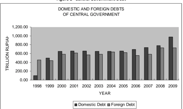
to cover deficit the state budget. The government debt increased to three to four-fold and almost three-quarters of those is domestic debt for bank restructuring (Boediono, 2009).

Figure 1 Central Government Debt

DOMESTIC AND FOREIGN DEBTS OF CENTRAL GOVERNMENT

0.00 200.00 400.00 600.00 800.00 1,000.00 1,200.00

1998 1999 2000 2001 2002 2003 2004 2005 2006 2007 2008 2009

YEAR

T

R

IL

L

IO

N

R

U

P

IA

H

Domestic Debt Foreign Debt

Source: Debt Management Office, Ministry of Finance, Republic of Indonesia

In recent years, new financing from both foreign and domestic financial resources are still required to meet the expenditure needs.The interest rate and amortization payments (about 30 percent of the total outlay) severely limit to the fiscal space. The state budget problems then shifted from the stimulus to fiscal sustainability (Rahmany, 2004). Conceptually, the state budget is said to be sustainable if it has the ability to finance all spending in the long term without endangering budgetary functions (see for example: Langenus, 2006; Yeyati and Sturzenegger, 2007).

The issue of the sustainability is an integral part of the discussion of the government's long-term ability to repay debt (Brixi and Mody, 2002). To maintain the fiscal solvency, the surplus of the state budget is a must (Chalk and Hemming, 2000). The main problem of the Indonesian budget sustainability is the existing deficit. The Law No. 17/2003 article 12 states that the deficit and total debt ratios are no more than 3 and 60 percent respectively. The question is then how to keep the budget deficit at a safe level so that the deficit can be financed.

38

investment (McKinnon, 1973; Shaw, 1973). Similarly, the foreign financed budget deficit is characterized by persistent exchange rate depreciation, balance of payment distress, and high inflation (Fry, 1988). Eventually, the debtor country experiences unstable economic growth.

This paper attempts to assess the fiscal sustainability and fiscal solvency and its relation to financial system stability in the case of Indonesia. The rest of the paper is organized as follows. First, the conceptual framework of fiscal sustainability will be reviewed. The next section presents the previous empirical studies. The research methods are delivered in the fourth section. The results of estimation are presented in the discussion below. Finally, the concluding remarks are drawn.

2. Literature Review

Macroeconomic literature introduces three definitions of fiscal sustainability. The first approach is based on the accounting rules that connect the options of financing government spending (G). If the domestic revenue, R, is not sufficient to cover G, the available financing option is debt (D) and money printing (seigniorage, S).

(Rt – Gt) = Dt + St (1)

The existence of seigniorage implies the relationship between monetary and fiscal policies.

The debt accumulation in the next period (t +1) will be D itself plus the interest rate (r):

Dt+1 = (1 + r) Dt + (Rt – Gt) + St (2)

The term of (R – G) is the primary balance (PB), total government expenditures excluding the interest rate payments. It can be rewritten as:

Dt+1 – Dt≡ ∆ Dt = r Dt-1 – PBt + St (3)

According to the accounting approach, the state budget sustainability can be achieved if there is no debt. Even if the government takes debt, the fiscal sustainability can be maintained as far as the additional debt must be proportional to the PB surplus (Dihn, 1999).

Equation (3) if disclosed further in the relative form to national income (Y) will be

39

In this context, the fiscal sustainability holds if the current primary balance position increases greater than the increase in the debt ratio (Ouanes and Thakur, 1997).

The second definition of fiscal sustainability is explained by linking to the solvency. Based on (4), ratio to Y requires that the rate of growth of Y should be taken into account. If the income increases constantly (suppose at g percent overtime), the additional debt will be:

t t t

t RD RBP S

g g r

RD − +

+ − =

∆ −1

1 (5)

When there is no new additional debt (∆ RDt = 0), then,

t t t

t RD S

g g r RPB + + −

= −1

1 (6)

In this case, budget surplus is required to attain fiscal solvency if the real rate of interest exceeds output growth, i.e., (r–g) > 0. The public sector has to make debt service payment at least equal to PB, or equivalently, it should have a primary surplus equal to PB. A primary fiscal surplus less than that amount (or a primary fiscal deficit) in that case implies perpetual public sector borrowing and debt accumulated indefinitely. For a country whose rate of output growth exceeds the real rate of interest, (r–g) < 0, incurring a primary deficit is till consistent with solvency. However, a deficit higher than PB implies that the country is moving away from a fiscal solvency position.

The third definition of fiscal sustainability is based on the accounting approach by imposing discount factor onto the equation (2):

{

}

k

t D PB S

r

D − +

+

=

∑

1 (

1

(7)

The limit value for an infinite time of the first term in equation (7) will be asymptotically equal to zero. The equation remains

{

}

k

t PB S

r

D − +

+

=

∑

) 1 (

1

(8)

40

Some different concepts discussed above have been inspiring a lot of researchers to assess fiscal sustainability. Hamilton and Flavin (1986) started the question of whether the deficit is still taking place in the control of long-term sustainability. They use the fixed interest rate to analyze US data. Wilcox (1989) extended Hamilton and Flavin approach by assuming interest rates are no longer fixed. The results of both studies show that US debt remains sustainable as far as the interest rate fluctuations are stationary.

Besides interest rates, some researchers began identifying some other factors. Buiter (1993) identified a high inflation rate will increase the primary deficit by reducing the value of real tax revenue. As a result, debtor countries have difficulties to conduct their fiscal operations. Consequently, adjustment period of debt maturity with tax revenue (e.g. tax smoothing) would be a feasible solution for fiscal sustainability realization (Barro, 1997).

Buiter (1997) further identified other factors that also affect to fiscal sustainability. He proposed the exchange rate, foreign exchange reserves, consumption expenditure, and government investment spending. Chouraqui, Hagemann, and Sartor (1999) emphasized the importance of fiscal policy consistency. Under the complexity of fiscal policy circumstances, Buiter (2002) suggested that the government debt is used only for investment spending. Meanwhile, the incremental tax revenue should be a constant fraction of the GDP.

In connection with the exchange rate, Turner (2002) noted the demand for Dollar-denominated bonds will increase when the monetary authority applied the free exchange rates regime. This is due to the confidence to the exchange rates in emerging markets is generally quite low. Calvo (2003 and 2004) found an interesting example of the economic impact generated by fiscal burden in Mexico. Mendoza and Oviedo (2004) pioneered the analysis of external debt sustainability by introducing the natural debt limit to consolidate fiscal burden.

Some similar studies in the case of developing countries have been conducted, for example by Yamauchi (2004) for Eritrea, Yilanci and Ozcan (2008) for Turkey, and Makin (2005) for the Southeast Asian countries. Meanwhile, the research conducted in Indonesia on domestic debt is still rare. This may be because the government bond market effectively began in 2001. Automatically, most of the research is devoted to assess economic impact of external debt (see for example: Kuncoro, 1999 and Saleh, 2002).

41

Ulfa and Zulfadin (2004) obtained ambiguous results. Some fiscal policies (i.e. budget reforms) reduce the sovereign debt. On the other hand, some fiscal policies (i.e. blanket guarantee) enlarge the contingent liabilities. Hanni (2006) examined some factors influencing the fiscal sustainability. The results of her study concluded that some external macroeconomic variables become the key determinants for achieving fiscal sustainability. Unfortunately, she did not incorporate the oil price in her analysis. Jha (2009) found that the oil price has a significant effect to the sustainable state budget related to the subsidies liabilities.

Recent studies have been conducted directly to analyze the vulnerability of state budget in relation to the debt burden. Ciarlone and Trebeschi (2006) observed the sovereign debt in the developing countries. They found that the key determinants identified above failed to predict the debt crisis. Tunner and Samake (2006) found that the probability of fiscal vulnerability can be reduced by fiscal adjustment programs. Celasun, Debrun, and Ostry (2007) analyzed the probability of fiscal vulnerability in 5 developing countries. The most interesting result is that the fiscal policy itself is the source of fiscal vulnerability risks.

3.

_{Research Method}

Many studies above suggest some important things. First, the external factors appear to be more dominant in influencing a country's fiscal condition. Second, so far there is no study in Indonesia yet, which integrates all of the external factors. This study closes the empirical fiscal policy gap in Indonesia, first, by synthesizing them. According to equation (5) and (6), the basic model of the Indonesian fiscal sustainability can be simply written as:

∆ RDt = f ( r, g, RDt-1, RPBt,, St ) (9a) ∆ RPBt, = f ( r, g, RDt-1 RPBt-1, St ) (9b)

Equation (9) is a VAR (vector auto regression) model. Associated with two kinds of debt, the relative interest rates covering the domestic interest rates [SBI (Sertifikat Bank Indonesia/Central Bank of Indonesia Certificate)] and the foreign interest rates (r) will be displayed. The depreciation (DEP), inflation rates (inf), and oil price (OP) are also used as explanatory variables. The detailed model is the fiscal policy reaction function:

∆ (RD)t = a1 + b1 (RD)t-1 + c1 (PRB)t + d1 St + e1 (SBI/r)t

+ f1 (EG)t + g1 (inf)t + h1 (DEP)t + i1 (OP)t + µt1 (10a)

∆ (RPB)t = a2 + b2 (RD)t-1 + c2 (PRB)t-1 + d2 St + e2 (SBI/r)t

42

The second significant contribution of this study is that unlike the previous studies in Indonesia (which generally used annual data), the two models are estimated with quarterly data during the post-crisis period (1999-2009). In general, the data obtained from Central Bank of Indonesia, Ministry of Finance, and the Central Board of Statistics. The data for this study have already been available on a quarterly basis except the primary balance. The data is then interpolated linearly from annual basis to fit the other data on the model. The primary balance is calculated as ratio to GDP.

Variables that will be used are specified as follows. Debt that is analyzed here is the central government debt only (excluding Central Bank of Indonesia, state-owned enterprises, or local government debts). The foreign debt is stated as net adjusted by principal payment and denominated in million US dollar. To convert to Indonesian currency (Rupiah), I use the official exchange rate issued by Central Bank of Indonesia. The domestic debt comprises short and long term debts and stated in trillion Rupiah. Eventually, we can derive the total debt as ratio to GDP.

United State Federal interest rate is used as the representative foreign interest rates. The three-months-SBI interest rate is treated as domestic interest rates. The two types of interest rates are presented in percent. Depreciation is calculated as a percentage change of the Rupiah against the US Dollar. Similarly, economic growth is calculated as the percentage change in GDP at constant prices in 2000. Inflation rate is derived from the GDP deflator that is ratio nominal GDP (in trillion Rupiah) to constant price GDP. The latest is also used to convert all variables into the real values. The difference of narrow money (M1) percentage supply growth and inflation rate (in percent) is used to identify seigniorage.

4.

Empirical Results

43

Table 1 Unit Roots Tests

Variable to be tested

Level First Difference

ADF PP ADF PP

RD -1.68840 -0.42020 -3.83114 -6.61046

SBI/r -2.58531 -3.79961 -4.67294 -4.67465

EG -4.66726 -34.01257 -4.31966 -34.57212

DEP -10.36075 -2.90569 -10.19866 -23.61770

INF -32.00175 -24.25623 -40.19748 -48.79715

OP -0.90323 -1.41771 -5.46118 -7.71728

S -14.79170 -12.95467 -7.91940 -42.58043

RPB -1.70075 -1.24309 -4.04858 -4.10342

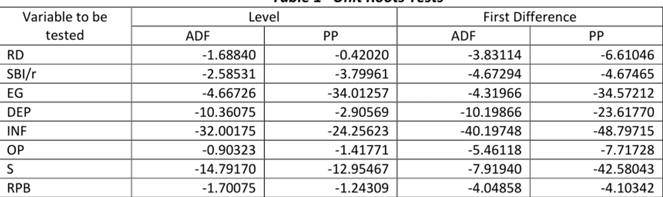
At the level data, the series of SBI/r, EG, DEP, INF, and S have a unit roots at 95 percent level of confidence. At the first difference data, all of variables under study have a unit roots. Their t-statistics values are much greater than the critical value at 5 percent significance. They imply that the series data are stationary at the first difference [I(1)] and the behavior of the variables vary around to the mean value and invariant overtime (Enders, 2004).

The second conditional method identifying fiscal sustainability and solvency is to apply Johansen’s co-integration test on equation (10). The result is summarized in Table 2. Using rank test of eight variables, the trace statistics value rejects the null hypotheses at 5 percent level. The result implies that they are the co-integrated variables even though they are not at the same degree of stationary. In other words, all of series data have a long-run relationship. As a consequence, they can be modeled as specified before to find out parameter estimate using empirical data.

Table 2 Multiple Cointegration Test

Trend assumption: Linear deterministic trend Series: RD SBI/R EG DEP INF OP S RPB Lags interval (in first differences): 1 to 1 Unrestricted Cointegration Rank Test

Hypothesized Trace 5 Percent 1 Percent

No. of CE(s) Eigenvalue Statistic Critical Value Critical Value

None ** 0.857517 290.1384 156.00 168.36

At most 1 ** 0.731765 208.2999 124.24 133.57

At most 2 ** 0.673109 153.0325 94.15 103.18

At most 3 ** 0.562910 106.0710 68.52 76.07

At most 4 ** 0.527858 71.3111 47.21 54.46

At most 5 ** 0.416192 39.7911 29.68 35.65

At most 6 * 0.192177 17.1875 15.41 20.04

At most 7 ** 0.177834 8.2241 3.76 6.65

44

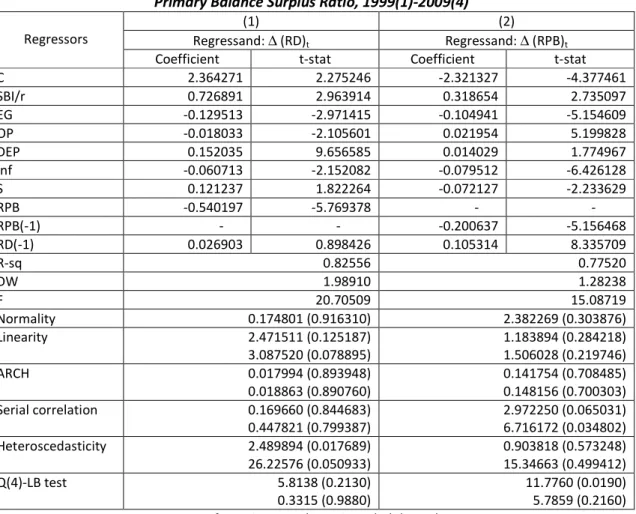
The estimation results of Indonesian government debt and primary balance change levels are presented in Table 3. The debt stocks in the previous periods are not able to explain change in debt ratio in the current period. On the other hand, they significantly can affect to the change in primary balance surplus for about 0.1 percent. In the opposite direction, the primary balance surplus contributes to the decrease in debt for about 0.6 percent. Those findings suggest that central government actively creates surplus to anticipate the sovereign debt in the future.

Table 3 Estimation Results of Changes in Total Government Debt Ratio and Primary Balance Surplus Ratio, 1999(1)-2009(4)

Regressors

(1) (2)

Regressand: ∆ (RD)t Regressand: ∆ (RPB)t

Coefficient t-stat Coefficient t-stat

C 2.364271 2.275246 -2.321327 -4.377461

SBI/r 0.726891 2.963914 0.318654 2.735097

EG -0.129513 -2.971415 -0.104941 -5.154609

OP -0.018033 -2.105601 0.021954 5.199828

DEP 0.152035 9.656585 0.014029 1.774967

Inf -0.060713 -2.152082 -0.079512 -6.426128

S 0.121237 1.822264 -0.072127 -2.233629

RPB -0.540197 -5.769378 - -

RPB(-1) - - -0.200637 -5.156468

RD(-1) 0.026903 0.898426 0.105314 8.335709

R-sq 0.82556 0.77520

DW 1.98910 1.28238

F 20.70509 15.08719

Normality 0.174801 (0.916310) 2.382269 (0.303876)

Linearity 2.471511 (0.125187)

3.087520 (0.078895)

1.183894 (0.284218) 1.506028 (0.219746)

ARCH 0.017994 (0.893948)

0.018863 (0.890760)

0.141754 (0.708485) 0.148156 (0.700303)

Serial correlation 0.169660 (0.844683)

0.447821 (0.799387)

2.972250 (0.065031) 6.716172 (0.034802)

Heteroscedasticity 2.489894 (0.017689)

26.22576 (0.050933)

0.903818 (0.573248) 15.34663 (0.499412)

Q(4)-LB test 5.8138 (0.2130)

0.3315 (0.9880)

11.7760 (0.0190) 5.7859 (0.2160)

Notes: figure in parentheses is probability value

45

On the other hand, economic growth and inflation rate have a negative impact on the change in central government debt as well as the primary balance surplus in the state budget. These are just the consequence of the ratio to the GDP and also the real terms. However, the increase in economic growth might reduce the debt and then the primary surplus. Similarly, maintaining the inflation rate will reduce the debt and then the primary surplus.

Furthermore, the oil price has a negative influence on the debt but a positive impact on the primary surplus. As a net oil importer country, Indonesia faces the dilemma when the oil price increases. In one hand, the central government revenue increases substantially. On the other hand, the central government has to spend more subsidies to avoid the increase of domestic fuel prices. However, this finding supports to the Jha’s study (2009).

The financial magnitude i.e. seigniorage also significantly influence both on debt and primary balance surplus ratios in the opposite directions. One percent increase in seigniorage tends to reduce primary balance ratio for about 7 percent and push increasing debt ratio for about 12 percent. It is notable that seigniorage here is measured by narrow money (M1). When we replace it into broad money (M2), the regression coefficients become smaller. This proves that the financial deepening and broadening is a good instrument to affect the fiscal position.

The last variable is depreciation. The depreciation Rupiah against the US Dollar could deteriorate both the debt and primary balance surplus. One percent depreciation of Rupiah tends to jeopardize the debt accumulation and surplus for about 0.15 and 0.01 percent respectively. It seems that stabilizing the exchange rate is a necessary condition for central government to maintain the soundness of state budget. This finding is similar and confirms to the study of Soelistijaningsih (2002) and Mark (2004).

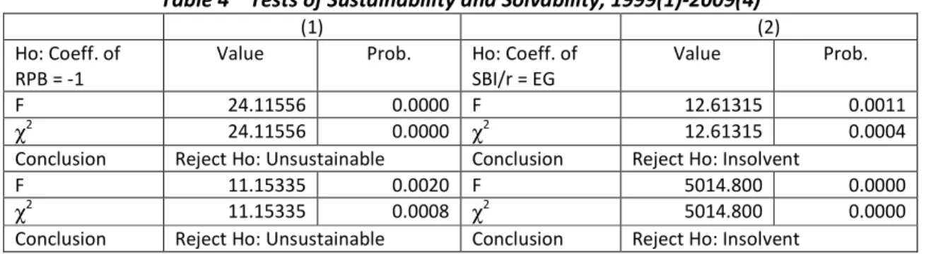
The third method to evaluate the fiscal sustainability and solvency is imposing directly some restrictions to the estimation results. Based on the equations (5 and 6), the state budget is said to be sustainable when the coefficient of PRB statistically equals -1 (or similarly the coefficient of RD in equation (6) statistically equals 1). According to the same equations, the state budget is said to be solvent if (r-g) statistically equals zero. The test is done empirically on equations (10) by carrying out the ANOVA (F) and χ2 procedures to prove whether the requirements are satisfied.

46

The ultimate conclusion is that the state budget is illiquid to undertake the debt payment in the future. The test results above give an important message that the state budget is very vulnerable in the context of fiscal risk occurrence. The important point here is that, in the adverse macroeconomic fluctuation and fiscal environment that faces the central government, solvency has as much to do with what might happen as what is expected to happen.

Table 4 Tests of Sustainability and Solvability, 1999(1)-2009(4)

(1) (2)

Ho: Coeff. of RPB = -1

Value Prob. Ho: Coeff. of SBI/r = EG

Value Prob.

F 24.11556 0.0000 F 12.61315 0.0011

χ2

24.11556 0.0000 χ2 12.61315 0.0004

Conclusion Reject Ho: Unsustainable Conclusion Reject Ho: Insolvent

F 11.15335 0.0020 F 5014.800 0.0000

χ2

11.15335 0.0008 χ2 5014.800 0.0000

Conclusion Reject Ho: Unsustainable Conclusion Reject Ho: Insolvent

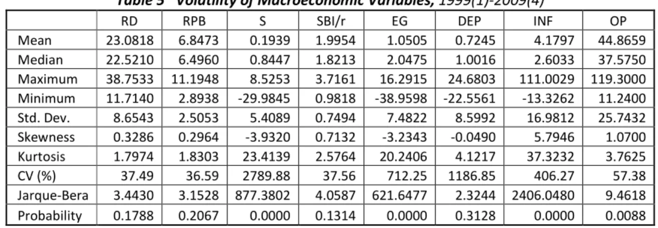
The third significant contribution of this study is that the sustainability of state budget is assessed the vulnerability of all explanatory variables. Table 5 summarizes the volatility of macroeconomic variables under the study. Seigniorage, depreciation, economic growth, and inflation rates are the most volatile indicated by the high coefficient of variation (CV). The higher CV is the higher risk. They imply that the state budget probability to be unsustainable and then insolvent is much higher.

In order to take into account the macroeconomic fluctuation above, in the next section, we will explore the direct reaction function between both variables simultaneously using vector auto-regression. The impulse responses of macroeconomic volatility on debt and primary balance ratios are graphically described in Figure 2. We assume that the ordering of the equations is as follows: exchange rate, GDP growth rate, seigniorage, inflation, oil price, interest rate, primary balance, and debt shocks. This order implies that debt affects all the variables contemporaneously, while exchange rate changes take effect with a lag. An inspection of these impulse response functions indicates that this ordering yields a reasonably satisfactory description of debt dynamics*).

*)

47

Table 5 Volatility of Macroeconomic Variables, 1999(1)-2009(4)

RD RPB S SBI/r EG DEP INF OP

Mean 23.0818 6.8473 0.1939 1.9954 1.0505 0.7245 4.1797 44.8659 Median 22.5210 6.4960 0.8447 1.8213 2.0475 1.0016 2.6033 37.5750 Maximum 38.7533 11.1948 8.5253 3.7161 16.2915 24.6803 111.0029 119.3000 Minimum 11.7140 2.8938 -29.9845 0.9818 -38.9598 -22.5561 -13.3262 11.2400 Std. Dev. 8.6543 2.5053 5.4089 0.7494 7.4822 8.5992 16.9812 25.7432 Skewness 0.3286 0.2964 -3.9320 0.7132 -3.2343 -0.0490 5.7946 1.0700 Kurtosis 1.7974 1.8303 23.4139 2.5764 20.2406 4.1217 37.3232 3.7625 CV (%) 37.49 36.59 2789.88 37.56 712.25 1186.85 406.27 57.38 Jarque-Bera 3.4430 3.1528 877.3802 4.0587 621.6477 2.3244 2406.0480 9.4618 Probability 0.1788 0.2067 0.0000 0.1314 0.0000 0.3128 0.0000 0.0088

48

Figure 2 Impulse Responses of Debt Ratio and Primary Balance Ratio

-1.5 -1.0 -0.5 0.0 0.5 1.0 1.5 2.0 2.5

5 10 15 20 25 30 35 40

RD RPB

Response of RD to Cholesky

One S.D. Innovations

-.6 -.4 -.2 .0 .2 .4 .6 .8

5 10 15 20 25 30 35 40

RD RPB

49

Figure 2 also displays the impulse response from an increase in the debt ratio. The innovation from an increase in the debt shocks results in a transitory appreciation in the exchange rate and transitory reduction in the interest rate. While the initial responses are difficult to reconcile intuitively, the simulations show that the subsequent increase in the interest rate, deterioration in GDP growth rate, and other economic deterioration result in a persistent increase in the primary balance to GDP ratio. The net effect on the primary balance path implied by the shock to all of macroeconomic variables, given the initial conditions, is a steady increase in the primary balance ratio for up to 32 quarters after the initial shock.

The co-movements observed in the variables of primary balance surplus and the debt dynamics are consistent with a priori expectations. The innovations to the primary balance and the oil price have the largest impact on the debt dynamics, followed by the innovation to economic growth, interest rates, inflation, seigniorage, and the real exchange rate. On the contrary, the innovations to the debt ratio and the oil price have the largest impact on the primary balance dynamics, followed by the innovation to economic growth, interest rates, inflation, seigniorage, and the real exchange rate. To sum up, in order to be sustainable and solvable, the Indonesian state budget approximately needs at least ten years.

In the next ten years, the state budget will face some challenges regarding the risky macroeconomic situation. The fiscal risks have to be explicitly disclosed as an integral part of the state budget (Barnhill and Kopits, 2003). Consequently, in order to realize fiscal sustainability and solvency, the implication for financial system is that the issuance of government bonds should be prudent considering the excessive burden in the future.

In terms of foreign debt, the debt burden can be shifted through rearrangement, rescheduling, and debt restructuring so that the sovereignty can be distributed in accordance with maturity. These foreign debt expenses also need to be synchronized with the burden of domestic debt maturity. In such case, the central government can use the swap mechanism to hedge the change in oil prices, foreign exchange rate, inflation rate, economic growth, and interest rate risks.

In term of domestic debt, the monetary authority could conduct some policies to mobilize domestic financial resources so the cost of fund is lower. The stronger secondary market of government securities is necessary condition to develop. On the other hand, financial deepening and broadening is sufficient condition to achieve financial system stability.

50

The ratio of the government foreign debt did show a declining trend. This moment needs to be utilized as well as possible in order to minimize the remaining risks. However, the lower debt ratio does not mean there have been increasing the government's financial position (Subyantoro, 2008). This is due to the possibility of state company’s divestment, depletion of public ownership resources of, and a decrease in government fixed capital. Another possibility is seeking a new debt, especially outside the state budget to cover old debts with the same amount. In addition, the quasi-fiscal activities of Central Bank of Indonesia, state enterprises, and local government’s enterprises can be a contingent liability if they are not managed correctly.

5. Concluding Remarks

This paper has provided an empirical evidence of the fiscal sustainability in the case of Indonesia. The main findings are Indonesian state budget has not been achieved both sustainability and solvency. The high fiscal risk is the main source. The lessons to be learned are as follows. First, effective identification of all fiscal risks is a prerequisite for their disclosure and management, and contributes to a fully informed conduct of fiscal policy. It requires a clear allocation of responsibilities among various parts of the public sector in assessing and reporting fiscal risks, as well as putting in place procedures to ensure that the entity playing the key role in determining fiscal policy has access to all relevant data.

Second, comprehensive disclosure of all fiscal risks helps facilitate identification and management of risks, and reduce borrowing costs in the long run. However, disclosure practices should be designed in ways that avoid engendering moral hazard from the perception of an implicit guarantee or harming the state’s economic interests. There is merit in reporting fiscal risks in a single document, such as a Statement of Fiscal Risks to be presented with the annual budget, and provides advice on its possible content.

Third, fiscal risk mitigation includes -- in addition to sound macroeconomic and public financial management policies -- practices that require justification for taking on fiscal risks and risk-sharing with the private sector. It may also involve use of insurance and hedging instruments, which so far remains limited but may increase as markets for innovative instruments develop further.

51

and ceilings on total issuance of guarantees may need to be subjected to parliamentary approval during the budget process.

Acknowledgement

I am greatly thankful to anonymous referees for the supports and constructive comments they have provided during the revising of this paper. I also acknowledge the support and useful suggestions of Andreea Maria Stoian, the editor of RJFP.

References

Barnhill, T.M. and G. Kopits. 2003. Assessing Fiscal Sustainability under Uncertainty. IMF Working Paper.

Barro, R., 1997. Optimal Management of Indexed and Nominal Debt. NBER Working Paper, No. 6197.

Boediono, 2009. Ekonomi Indonesia Mau ke Mana?, Kumpulan Esai Ekonomi (Indonesian Economy, where does it go?, Compedium of Economic Essays). KPG & Freedom Institute, Jakarta.

Buiter, W.H., 1993. Public Debt in the USA: How Much, How Bad, and Who Pays?. NBER Working Paper, No. 4362.

Buiter, W.H., 1997. Aspects of Fiscal Performance in some Transition Economies under Fund – Supported Programs. IMF Policy Discussion Paper.

Buiter, W.H., 2002. The Fiscal Theory of the Price Level: A Critique. Economic Journal.112(127), pp: 459-80.

Celasun, O., X. Debrun, and J.D. Ostry, 2007. Primary Surplus Behavior and Risks to Fiscal Sustainability in Emerging Market Countries: A “Fan-Chart” Approach. IMF Working Paper.

Chalk, N., and R. Hemming, 2000. Assessing Fiscal Sustainability in Theory and Practice. IMF Working Paper.

Chouraqui, J.C., R.P. Hagemann, and N. Sartor, 1999. Indicators of Fiscal Policy: A Reexamination. OECD Working Paper, No. 78.

Ciarlone, A. and G. Trebeschi, 2006. A Multinomial Approach to Early Warning System for Debt Crises. Banca D’Italia Working Paper, No. 588.

Cuddington, J.T., 1996. Analysing the Sustainability of Fiscal Deficits in Developing Countries. Economics Department Georgetown University. Washington, D. C.

Brixi, P.H. and A. Mody, 2002. Dealing with Government Fiscal Risk: An Overview. In: Government at Risk, The World Bank & Oxford University Press.

Cebotari, A., et. al., (2009). Fiscal Risk, Sources, Disclosure, and Management. Fiscal Affair Department, IMF, Washington D. C.

52

Enders, W., 2004. Applied Econometric Time Series. Second edition, John Wiley & Son, New York.

Fry, M.J., 1988. Money, Interest, and Banking in Economic Development. The Johns Hopkins University Press, Baltimore.

Geithner, T., 2002. Assessing Sustainability. IMF Working Paper.

Hamilton, J.D. and Flavin, M.A., 1986. On the Limitations of Government Borrowing: A Framework for Empirical Testing. American Economic Review, 76(4), September, pp: 808-19.

Hanni, U., 2006. Sustainabilitas Fiskal Indonesia dan Faktor-Faktor yang Mempengaruhinya (The Indonesian Fiscal Sustainability and the Influencing Factors). Jurnal Keuangan Publik, 4(2), September, pp: 19-37

Jha, S., 2009. Macroeconomic Uncertainties, Oil Subsidies and Fiscal Sustainability in Asia. ADB Research Paper.

Kuncoro, H., 1999. Dampak Kebijaksanaan Pengeluaran Pemerintah terhadap Pertumbuhan

Ekonomi Indonesia (The Impact of Government Expenditures Policy on Indonesian Economic Growth). Unpublished Thesis, UGM, Yogyakarta.

Langenus, G., 2006. Fiscal Sustainability Indicators and Policy Design in the Face of Ageing.

National Bank of Belgium Working Paper.

Makin, T., 2005. Fiscal Risk in ASEAN. Agenda, 12(3), pp: 227-38.

McKinnon, R.I., 1973. Money and Capital in Development. The Brooking Institution, Washington, D. C.

Mark, S.V., 2004. Fiscal Sustainability and Solvency: Theory and Recent Experience in Indonesia. Bulletin of Indonesian Economic Studies, 40(2), August, pp: 227-42.

Ouanes, A and S. Thakur, 1997. Macroeconomic Accounting and Analysis in Transition Economies. IMF, Washington D. C.

PPE UGM and BAF, 2004. Studi Manajemen Utang Luar Negeri dan Dalam Negeri Pemerintah dan Assessment terhadap Optimal Borrowing (Study on External and Domestic Debts Management and Assessment on Optimal Borrowing). Final report.

Rahmany, F.A., 2004. Ketahanan Fiskal dan Manajemen Utang Dalam Negeri Pemerintah (Fiscal Sustainability and Government Domestic Debt Management). In: Kebijakan Fiskal, Pemikiran, Konsep, dan Implementasinya (Fiscal Policy, Idea, Concept, and its Implementation), Kompas, Jakarta.

Saleh, S., 2002, Pengaruh Kebijakan Defisit Anggaran Pemerintah terhadap Perekonomian Indonesia (The Influence of Government Budget Deficit on Indonesian Economy). Unpublished Disertasion, UGM, Yogyakarta.

Shaw, E.S., 1973. Financial Deepening in Economic Development. Oxford University Press, New York.

53

Subyantoro, H., 2008. Adakah Persoalan Contingent Liabilities dan Fiscal Risk di Indonesia?: Sebuah Pelajaran yang Sangat Berharga (Are There any Contingent Liabilities and Fiscal Risk in Indonesia: Some Valuable Lessons). Professor speech, Universitas Borobudur, December, 23, Jakarta.

Tunner, E. and I. Samake, 2006. Probabilistic Sustainability of Public Debt: A Vector Autoregression Approach for Brazil, Mexico, and Turkey. IMF Working Paper.

Turner, P., 2002. Bond Markets in Emerging Economies: an Overview of Policy Issues. Bank for International Settlement, No. 11.

Ulfa, A. and R. Zulfadin, 2004. Seberapa Seriuskah Perhatian Indonesia terhadap Isu-isu Kontingensi Fiskal? (How Serious does Indonesia Pay Attention to Fiscal Contingency Issues?). Kajian Ekonomi dan Keuangan, 8(2), June.

Wilcox, D., 1989. The Sustainability of Government Deficits: Implications of the Present-Value Borrowing Constrain. Journal of Money, Credit and Banking.3, pp: 291-306.

Yamauchi, A., 2004. Fiscal Sustainability, the Case of Eritrea. IMF Working Paper.

Yeyati, E.L. and F. Sturzenegger, 2007. A Balance-Sheet Approach to Fiscal Sustainability. Universidad Torcuato Di Tella Working Paper.