Larsen, Legay, Nyman (Eds.): 1st Workshop on Advances in Systems of Systems (AiSoS 2013)
EPTCS 133, 2013, pp. 47–66, doi:10.4204/EPTCS.133.6
c
A. Arnold, B. Boyer, A. Legay This work is licensed under the Creative Commons Attribution License.
DANSE approach
Alexandre ARNOLD EADS Innovation Works
Toulouse, France [email protected]
Benoˆıt BOYER, Axel LEGAY INRIA - Rennes Bretagne Atlantique
Rennes, France [email protected]
This paper presents some of the results of the first year of DANSE, one of the first EU IP projects dedicated to SoS. Concretely, we offer a tool chain that allows to specify SoS and SoS requirements at high level, and analyse them using powerful toolsets coming from the formal verification area. At the high level, we use UPDM, the system model provided by the british army as well as a new type of contract based on behavioral patterns. At low level, we rely on a powerful simulation toolset combined with recent advances from the area of statistical model checking. The approach has been applied to a case study developed at EADS Innovation Works.
1
Introduction
While SysML [41], the Systems Modeling Language derived from UML [36], has been widely adopted for Systems Engineering applications, the specificities of Systems of Systems (SoS) fostered the creation of further customizations. The Unified Profile for DoDAF and MoDAF (UPDM) [37], based on the US and UK military architectural framework, is one of them and is used on a regular basis in SoS Engineering.
Specific extensions of SysML/UPDM are considered in DANSE[13], one of the first European project aiming at developing a methodological and technical framework for SoS Engineering with associated tool support. This framework shall support the SoS architect from the modeling activities to the analysis phase (abstraction, simulation, formal verification), especially by providing concrete solutions to address common SoS issues: constant evolution of a large-scale SoS and its stakeholders’ needs, unexpected emergent behaviors, limited awareness of the global situation...
In the frame of DANSE, we extend the language of SysML/UPDM to add formalized requirements for an SoS. Formalizing the SoS goals makes it possible to verify them automatically (with an adjustable probability) using a statistical model checker such as Plasma-Lab [24, 28] in combination with a simula-tion platform such as DESYRE. The challenge is to propose a high-level formal language that is directly usable by an SoS architect, while being still automatically translatable to the expressive low-level specifi-cation of the model checker, in a similar way to editors like IBM Rhapsody that could make an executable specification (FMI) out of a high-level formalism (SysML/UPDM behavioral diagram).
So we propose in this paper the very first contract language for SysML/UPDM, defined using a strong B-LTL based semantics, but close to hand written English requirements for SoS on the surface. This language of goal formalisation, which is developed in the scope of the DANSEproject, is called the Goal and Contract Specification Language (GCSL).
GCSL makes use of the Object Constraint Language (OCL), a formal language by the Object Man-agement Group (OMG) [34] used to describe static properties on UML models, thus also on SysML/UPDM ones. OCL can be used for a number of different purposes, but especially as a model-based query lan-guage and for writing expressions, which perfectly suits our needs here. GCSL also reuses the Contract Specification Language (CSL) [43], developed in the previous SPEEDS European project [44], which comes with convenient temporal patterns. The three key elements required for the formalization of behavioral goals and the way we address them in our approach are (1) being able to refer to model el-ements: use of the same names as in the SysML/UPDM model, (2) being able to write static properties about them: use of OCL and (3) being able to integrate these expressions inside behavioral patterns: use of CSL patterns.
After a short description of the SoS modeling in Section 2, this paper presents in Section 3 the GCSL based on the semantics of UPML modeling, thus we show how to translate the properties into B-LTL formulas (Section 4) into order to check them using the statistical model checking framework for SoS (Section 5). Finally, Section 6 illustrates the approach applied to the case study of DANSE.
2
System of Systems Modeling
Overview of SysML/UPDM
SysML [41] is a general-purpose modeling language defined as an extension of a subset of the Unified Modeling Language (UML) [36] using UML’s profile mechanism. SysML is used for Systems Engi-neering applications, whereas UML is more targeted towards object-oriented Software EngiEngi-neering. A large set of diagrams is provided with SysML to model a system’s requirements, structure (e.g. block definition diagram, internal block diagram), behavior (e.g. state machine, activity diagram), etc.
Using the same UML’s profile mechanism, another language built on top of UML/SysML has de facto become a standard for SoS architects: UPDM. This profile is the result of the unification effort of the US Department of Defense and the UK Ministry of Defense architecture frameworks and associated meta-models. It adds a layer of new meta-objects that are typically (but not exclusively) used in the context of military SoS, as well as a significant amount of predefined views (e.g. system views, operational views, capability views) which help splitting the whole modeling activity in smaller tasks.
The executable part of a UPDM modeling can be compiled into a program based on the Func-tional MockUp Interface (FMI) [40] that defines a standardized interface used in simulations of com-plex systems. In DANSE, the SoS is compiled into FMI program and executed by the simulation engine DESYRE [2]. This whole FMI program can be considered as a state transition system, e.g. the formal semantics on which we will use to propose our language. The states denote the global states of the SoS, e.g. the result of collecting the internal states of each constituent in the SoS. The transitions denote the actions and events that occur in the SoS and eventually modify the internal state of some system constituents and thus, the global state of the system.
Definition 1(State Transition Systems). Let X be a set of variables that are mapped to the values of D, the set of all possible values. We define S a set of states. Each state s is characterized by a mapping
• s0∈S contains the initial states of the system
• R⊆S×S is the transition relation. We use the more convenient notation s→s′to denote(s,s′)∈R.
All valid execution (or run) of a transition system is a sequence of states led by the R from any initial state. A run of length n will denoted asπ=s0;s1;s2;. . .;snwhere s0∈I and si→si+1holds for0≤i<n. Each transition system has a global clock, which is denoted by the variable t. We note ti=µsi(t), the
observed time value of t when the executed system reaches the state si. For any execution path the system is in state siwhen ti≤t<ti+1and the evolution of the time is monotonically increasing, e.g. ti<ti+1.
In the first year of the DANSEproject we limit ourselves to systems of systems who environment’s behaviors are fully known in advance (hence representable via state transition systems), like it is the case for most of adaptive systems studied in the litterature [48, 20, 8, 19]. The reason is that this corresponds to the current possibilities of the UPDM. In future work, we will study more complex aspects such as unknown environment, hence more complex dynamicity features. For this, we will first have to consider extension of the UPDM model.
Stochastic aspects of the model
Stochastic modeling is a way to describe behaviors that are not deterministic by nature, or to abstract a behavior that is simply too complex to be modeled explicitly (as white box). So it is typically very useful in a SoS context. Behavioural modeling in SoS examples such as an Emergency Response to a city fire typically shows numerous attributes/parameters that would not be deterministic, such as the time between two fires or the duration of an action performed by a human.
A first proposal of how to put stochastic data in the SysML/UPDM model has been integrated into the DANSEproject. It is based on a set of attribute stereotypes that can be applied to any block attribute. This idea is close to the suggestion of the non-normative distribution extensions made in appendix of the SysML 1.3 specification, but adds the possibility to regenerate a distribution-based random value whenever needed (and not only at initialization). This addition is important because even the same person does never perform the same task in the exact same amount of time, so that the duration of the task shall be recalculated every time.
Adding stochastic data to the SoS model implies of course that each simulation is likely to generate a different trace than the previous ones, and as a consequence that one run will not be enough to verify whether the SoS meets its requirements or not. This is why being able to automate this verification process in a mathematical way (provided the requirements are formalised) is a great support for the SoS architect when assessing a candidate architecture.
Since the SoS we consider exhibit some stochastic behaviors, each run has an associated probability of being executed. This probability is given by an unkonwn distribution due to the high complexity of the model: a system is designed by the paralell composition of components that may have a stochastic behavior.
3
A Contract Language for UPDM/SysML Requirements
Before defining the new contract language, we introduce the notion of contract for the SoS formalized as a stochastic state transition systems.
are properties about the execution of the system. Thus, a contract for the system specifies what the system shall ensure the promise when the system shall satisfy the assumption. The notation Sys|= (A,P)means that the contract(A,P)is satisfied by the system Sys. Relying on the state transition system semantics,
the satisfaction of a contract is
Sys|= (A,P) iff ∀π,π|=A⇒π|=P
whereπis a valid run of Sys andπ|=A (or P) means the runπ satisfies the assumption A (the promise P resp.).
For stochastic systems, it is generally more meaningful to quantify how a system satisfies a contract: this valuation is given by the probability that the system satisfies the contract. Intuitively, if the distribu-tion to execute each run of a given stochastic system is known, the probability that this system satisfies the contract is the sum of the probabilities of all the runs that satisfy the contract (see Section 5).
Definition 3(Contracts for Stochactic State Transition Systems). Let be a stochastic system Sys, a con-tract(A,G)and a threshold value k∈[0..1]. For the system Sys, we now consider the contract P∼k(A,G),
where∼∈ {<,≤,=,≥, >}and0≤k≤1. The contract is satisfied if and only if the relation holds, e.g. if the probability p of Sys|= (A,G)satisfies the relation p∼k.
In this work, for efficiency reasons, we decided to estimate the probability pusing statistical model checking rather than computing it with a numerical approach such as Prism [39]. Another reason to use SMC is that it relies on monitoring traces, hence it allows to verify properties that cannot be expressed in classical logics. In this paper, this aspect will not be explored, but it is a main topic of DANSE. SMC consists in verifying the property (here contract) against several simulations of the system. Then, an algorithm from the statistic area is used to estimate the probability to satisfy the property. The contract to monitor is translated into a B-LTL formula (see Section 4) that characterizes a set of simulation traces. Thus, the simulation monitoring consists of observing each simulation to decide if the B-LTL formulas holds or not.
We now introduce the language to express the assumptions and promises dedicated to the System of Systems. The GCSL syntax for patterns is a combination of the Object Constraint Language (OCL) and the contract patterns of the CSL `a la ”SPEEDS” [44]. The SPEEDS contract specification patterns are introduced in the SPEEDS Deliverable D.2.5.4 ”Contract Specification Language (CSL)” [43] and used to give a high-level specification of real-time components. They have been introduced to enable the user to reason about event triggering that are equivalently replaced in DANSEby property satisfaction. The properties handled by these patterns are about the state of a SoS. We use OCL to specify these state properties. This language allows to build some behavioral properties to express some temporal relations about facts or events of the system denoted by the state properties. It is sufficiently powerful to describe precisely a state of a SoS. Here, we will only consider a subset of the OCL language, but it is not unrealistic to consider a larger subset of OCL to describe the requirements. We restrict the language here to express some properties that can be verified using the SMC techniques applied to SoS’s.
We briefly recall the notion of Collection that we will use in the rest of the paper.
For example, the expressionSoS.itsFireStationsdenotes collection of all the instances of type
FireStation at state σ. OCL defines some operators that can be applied to any collection: SoS.
itsFireStations→size()counts the number of instances of typeFireStation. The most impor-tant feature of the collection is the predicates we can define using quantification:
• SoS.coll→forAll(x|φ(x)) denotes that for all element x, which belongs to the collection
SoS.coll, the propertyφ(x)holds.
• SoS.coll→exists(x|φ(x)) denotes for that there exists one elementx, which belongs to the collectionSoS.coll, the propertyφ(x)holds.
State properties in OCL
Originaly introduced to supplement UML, the Object Constraint Language (OCL) [35] is particularly adapted to describe the internal state of a component. The Object Constraint Language is a rather simple-to-write, yet formal text language that provides constraint and object query expressions based on any meta-model, so for instance the SysML/UPDM ones. It has a concise notation for accessing, collecting, filtering and evaluating model elements. More generally, it allows to write invariants on a model, that we use in our approach to write the static properties that we insert in the behavioral contracts. As we will see in the following paragraphs, we also pushed the concept further by sometimes embedding a CSL pattern inside an OCL-like expression, when we want to state that the pattern shall hold for some or all elements in a set. We recall some OCL notations used in the rest of the paper, but the reader can find the whole specification in [35]. Components store internal values into attributes that are denoted by the standard dot-syntax. For example, the number of people in the district 1 atσ, the state reached by the SoS, isdistrict1.population. More particular to OCL, it is also possible to define a collection of attributes using the same syntax: the expressionSoS.itsDistricts.population→sum()denotes the number of total people. For the sake of clarity in the rest of the paper, we only focus on theCollection
type without considering all its refinements (Set, Ordered Sets, . . . ), and the subset of Boolean and arithmetic expressions over the attributes of the SoS’ component instances.
The behavioral patterns
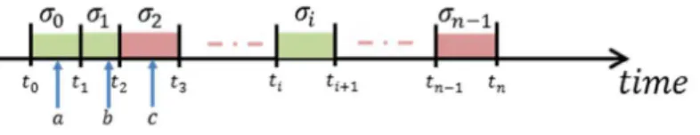
The semantics of the patterns is based on the satisfiability of any predicate on the whole set of execution paths that defines the pattern, which the definition of the following patterns are based upon. Consider the state propertyΨand a time value sequencet0,t1, . . . ,tnthat defines the state sequenceσ0,σ1, . . . ,σn such thattiis the time value where the system reachesσi. In other words, the system is in stateσi when ti≤time<ti+1.
Figure 1: Satisfaction ofΨduring an execution path.
time interval[t0,tn). If we finally consider any the time ticksa,bandc, Ψholds during[a,b]but does
not during[a,b]nor[b,c]and the occurrence number ofΨis 1 in[a,b],[a,c]or[b,c].
We define some selected patterns, but the more exhaustive list can be found in Appendix B. These patterns proved very useful for SoS applications. We assume thatΨandΨiare state properties anda,b,c are time constants such that the time intervals defined in the patterns are valid.
wheneverΨ1occursΨ2does not occur during following[a,b]
This pattern specifies thatΨ2is never satisfied during the relative interval[a,b]afterΨ1, i.e. ¬Ψ2
holds during[a,b]. By relative we means that whenΨoccurs att, the relative interval corresponds
to[a+t,b+t].
WheneverΨ1occursΨ2occurs within[a,b]
The constraintΨ2must be satisfied at least once during[a,b]afterΨ1.
Ψduring[a,b]impliesΨ1during[a,c]thenΨ2during[c,b]
WheneverΨholds during[a,b]there exists a split atcof[a,b]such thatΨ1holds during[a,c]then
Ψ2holds during[c,b].
The CSL patterns are originally designed to specify the behavior of any component instance by to-tally abstracting its environment without quantification. It is not possible to specify a contract about the interaction between two anonymous components. By anonymous, we mean that no particular instance is explicitly referenced by the component identifier. Let us consider a SoS with a set of components
Districtand twoDistrictpropertiesPsi1andΨ2in OCL. The patterns allow to express the behav-ioral property for some explicit component, e.g.Whenever[Ψ1(district1)]occurs[Ψ2(district1)]
occurs within [a,b], it is not possible to generalize the behavioral property to any Districtof the system, e.g. a property like ”For alldistrict, Whenever[Ψ1(district)]occurs [Ψ2(district)] occurs within[a,b]”.
To overcome this important limitation, we extend the proposed grammar (see Appendix B) by over-lapping the patterns with the OCL collection predicates, e.g. forAll(x|...) andexists(y|...). Then, the generalized behavioral property presented below is now:
SoS.itsDistricts→forAll(district|
Whenever[Ψ1(district)]occurs[Ψ2(district)]occurs within[a,b])
Using these OCL predicates for quantify the patterns keep the language not so different in comparison with the original OCL, except we restrict the nesting capability. The OCL syntax allows to nest the quantification without any limit. If there is no theoretical reasons to have limit, we impose a limit of 2 nested quantifications in our language. From the verification point of view, a behavioral formula with more nested quantifications is not practically check-able. Moreover, we never need more to express the requirements of CEA incubator in DANSE. So we assume in the next, that the patterns have are of the formSoS.coll1→forAll(x|SoS.coll2→forAll(y|. . .Pattern(x,y). . .), wherePatternis any behavioral pattern.
Another important limitation of this combination OCL + patterns is the inability of express property about cumulative values during an execution path: to solve this problem we introduce the path operators
mean(),sum(),prod()to denote the value of a numerical expression: for example,mean(district1.
population)denotes the average value of the attribute district1.population) computed with the values obtained of the different state of the path.
Examples of Requirements
Table 1 illustrates the kind of properties that we will express with our language. We use syntactic coloring to distinguish the different parts of the language used in the property: the words in red are identifiers from the model, the blue part is from OCL and bold black keywords are temporal operators. These requirements show the capabilities of our language using different requirements of this use case. Whereas the requirement 1 is purely structural, the requirements 2 and 3 are relative to the execution of the SoS: the first one is written using strictly OCL, the second one shows the cumulative operators we introduced and the third one is defined with a behavioral pattern. The presented requirements are contracts without assumption or, more precisely, they are contracts with an assumption that is implicitly ”true”.
”Any district cannot have more than 1 fire station, except if all districts have at least 1” SoS.itsDistricts→exists(district|district.containedFireStations→size()>1) implies
SoS.itsDistricts→forAll(district|district.containedFireStations→size()≥1) ”The mean city area under fire shall be less than 0.01%”
mean(SoS.itsDistricts.fireArea→sum())≤0.0001
”The fire fighting cars hosted by a fire station shall be used all simultaneously at least once in 6 months”
SoS.itsFireStations→forAll(fireStation|
Whenever [fireStation.hostedFireFightingCars→exists(ffCar|ffCar.isAtFireStation)] occurs, [fireStation.hostedFireFightingCars→forall(ffCar|ffCar.isAtFireStation= false)]
occurs within [6 months])
Table 1: Examples of Requirements formulated in the CAE incubator
4
Translating Contracts into Bounded-LTL Formulas
Bounded Linear Temporal Logic
As said previously, the Bounded Linear Temporal Logic (B-LTL) is an extension of the Linear Temporal Logic (LTL) [11] in which each temporal operator is bound by a temporal constant. This Logic is such expressive that it covers precisely a large set of properties. It is particularly adapted to Statistical Model Checking (SMC) [47, 42]. The SMC principle is to monitor some simulations in order to check a B-LTL property and use the results from the statistics area (sequential hypothesis testing or Monte Carlo simulation) in order to decide whether the system satisfies the B-LTL property or not with some degree of confidence. Since the conducted simulations are finite, the infinite path semantics of LTL has no sense, whereas checking B-LTL formulas does.
The formulas are built using the standard logic connectors∧,∨, =⇒,¬and the common temporal modalitiesG, F, X,U over some atomic propositions. Each temporal modality is indiced by a bound defining the length of the run on which the formula must hold. The validation of a B-LTL formula against an execution path has a meaning only if the length of this path is enough to reach all bounds constituting the formula.
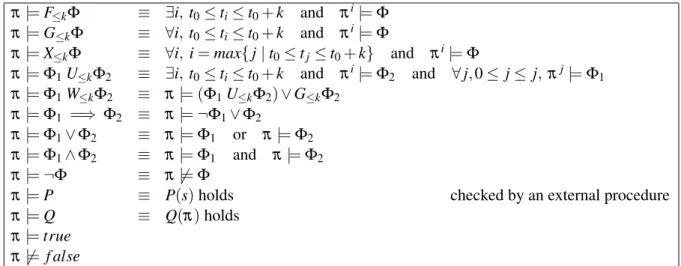
The atomic propositions used in the B-LTL formulas are build using some state predicates or run predicates. These predicates only require to be decidable for a given input, e.g. a state or a run section, and we assume this decision to be performed by an external procedure. Consideringπ=s0s1. . .sna finite run of a transition system andΦa B-LTL property,π|=Φmeans that the runπsatisfies the propertyΦ. The suffixsisi+1. . .sn ofπ is notedπi. Assumingk>0, a runπ=s0s1. . .sn, a state predicatePand a run predicateQ, the satisfiability of the B-LTL formulasΦ,Φ1andΦ2is defined in Table 2.
π|=F≤kΦ ≡ ∃i,t0≤ti≤t0+k and πi|=Φ
π|=G≤kΦ ≡ ∀i,t0≤ti≤t0+k and πi|=Φ
π|=X≤kΦ ≡ ∀i,i=max{j|t0≤tj≤t0+k} and πi|=Φ
π|=Φ1U≤kΦ2 ≡ ∃i,t0≤ti≤t0+k and πi|=Φ2 and ∀j,0≤ j≤ j,πj|=Φ1
π|=Φ1W≤kΦ2 ≡ π|= (Φ1U≤kΦ2)∨G≤kΦ2
π|=Φ1 =⇒ Φ2 ≡ π|=¬Φ1∨Φ2
π|=Φ1∨Φ2 ≡ π|=Φ1 or π|=Φ2
π|=Φ1∧Φ2 ≡ π|=Φ1 and π|=Φ2
π|=¬Φ ≡ π6|=Φ
π|=P ≡ P(s)holds checked by an external procedure
π|=Q ≡ Q(π)holds
π|=true
π6|= f alse
Table 2: Semantics of B-LTL
Overview of the translation procedure
As illustrated in the third example of requirements of Table 1 the language is layered as some behavioral properties defined using the patterns combined with some state properties written in OCL These behav-ioral properties can themselves be wrapped into an OCL collection expression to quantify the behavbehav-ioral properties over some constituents of the SoS. The translation of a contract will be made by translating from its assumption and its promise only the OCL quantification and the pattern layers. The translated property will be checked against some simulations. The state properties expressed in OCL have to be checked against some states and for them, no treatment is done during the translation. The state properties are kept in the translated formula and there will be dynamically checked. We assume that the satisfiability of the state properties is solved by an external procedure based on an existing OCL-checker [38].
Proposition 1. Let us consider a contract(A,P)of a given SoS and assume any simulation is bounded by k a maximum time of execution. If there exist two B-LTL formulas A′and P′such that A′(or P) and A (P′resp.) are equivalent for any k-bounded simulations, then the B-LTL formula A′ =⇒ P′is equivalent to the contract(A,P)for any k-bounded simulations.
The proof is a trivial consequence of Definition 2 written using B-LTL. Moreover, extending the translation to a stochastic contract is natural. The pair (A,P) of any stochastic contract is similarly
treated.
OCL quantification translation
OCL expressions occur at two levels within a pattern: as atomic propositions to define a state condition and as quantifications. The first case will be directly treated by an external OCL-checker against a state of the SoS or translated into a more generic semantics provided by the SMC-checker. But some atomic propositions can also contain some quantification about component collections and in this case they can also be processed as explained below. The second case is the most interesting case. The B-LTL logic has no quantification support; it could be extended but this needs to rewrite the B-LTL checker. Moreover, adding quantifications to the logic increases significantly the complexity of the satisfiablity decision.
Moreover, the instances of each component type are statically specified in the Internal Block Diagram (IBD) by the SoS architect. In the CAE incubator, the IDB is namedidbFireEmergencyand gives the list of all system constituents instantiated in the SoS: 10 districts, 1 fire headquarter, 3 fire stations and 7 fire fighting cars shared by the fire stations, etc. Since the number of constituents is known and finite in the SoS, any universal quantification (or an existential quantification) over a collection can be interpreted as a conjunction (a disjunction resp.). Using the CAE incubator and assuming a valid propertyφ for the fire stations, the propertySoS.itsFireStations→forAll(x|φ(x))is equivalent toφ(fireStation1)∧φ(fireStation2)∧φ(fireStation3).
In cases where φ contains also a quantification,φ must also be unfold. The generalization of the process is recursively defined as:
un f old coll→forAll(x|φ(x)
= ^
x∈coll
un f old φ(x)
un f old coll→exists(x|φ(x)
= _
x∈coll
un f old φ(x)
un f old expr) = expr, otherwise
Pattern translation
For the purpose of translation to B-LTL, we assume that the constantk, is an additional parameter given by the user: it corresponds to the execution time for which we expect the property hold. Whenever an unbound pattern to write a property like ”Always . . . ” is meaning full for the specification, statistical model checking still checks the B-LTL property against a simulation that is finite: kis used to replace the implicit unbound value of the property. Moreover, to be successfully translated, the pattern must be consistent: in particular the intervals must have correct bounds and intervals must be all visited before the end of the simulation (and so the constantk) is reached.
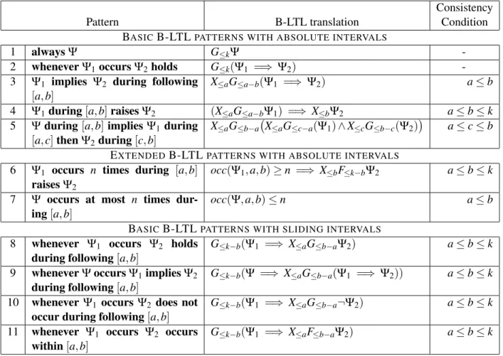
Proposition 2. AssumingΨ,Ψ1andΨ2denote some state propositions nested in a pattern P, e.g. OCL propositions, and a constant k>0then, for any run of length k, there exists a B-LTL formula equivalent to P. Table 3 summarizes the valid B-LTL translations.
Consistency
Pattern B-LTL translation Condition
BASICB-LTLPATTERNS WITH ABSOLUTE INTERVALS
1 alwaysΨ G≤kΨ
-2 wheneverΨ1occursΨ2holds G≤k(Ψ1 =⇒ Ψ2) -3 Ψ1 implies Ψ2 during following
[a,b]
X≤aG≤a−b(Ψ1 =⇒ Ψ2) a≤b
4 Ψ1during[a,b]raisesΨ2 (X≤aG≤a−bΨ1) =⇒ X≤bΨ2 a≤b≤k 5 Ψduring[a,b]impliesΨ1 during
[a,c]thenΨ2during[c,b]
X≤aG≤b−a X≤aG≤c−a(Ψ1)∧X≤cG≤b−c(Ψ2)
a≤c≤b
EXTENDEDB-LTLPATTERNS WITH ABSOLUTE INTERVALS 6 Ψ1 occurs n times during [a,b]
raisesΨ2
occ(Ψ1,a,b)≥n =⇒ X≤bF≤k−bΨ2 a≤b≤k
7 Ψ occurs at most n times dur-ing[a,b]
occ(Ψ,a,b)≤n a≤b
BASICB-LTLPATTERNS WITH SLIDING INTERVALS 8 whenever Ψ1 occurs Ψ2 holds
during following[a,b]
G≤k−b(Ψ1 =⇒ X≤aG≤b−aΨ2) a≤b≤k
9 wheneverΨoccursΨ1impliesΨ2
during following[a,b]
G≤k−b(Ψ =⇒ X≤aG≤b−a(Ψ1 =⇒ Ψ2)) a≤b≤k
10 whenever Ψ1 occurs Ψ2 does not occur during following[a,b]
G≤k−b(Ψ1 =⇒ X≤aG≤b−a¬Ψ2) a≤b≤k
11 whenever Ψ1 occurs Ψ2 occurs within[a,b]
G≤k−b(Ψ1 =⇒ X≤aF≤b−aΨ2) a≤b≤k
Table 3:Pattern mapping
Extended B-LTL patterns The patterns 6 and 7 require to count the number of occurrences in[a,b].
Counting is not possible by strictly using B-LTL. We assume that there exist a dedicated procedure occ(Ψ,a,b)that counts the number of times whereΨis satisfied and compare it to the valuen. We use
similarly some external treatment to evaluate the operatorssum(),mean(), . . . that compute a accumu-lated value of an expression during a time interval.
Sliding intervals the interval[a,b]to consider is located after timetat which the first part of the pattern ”WheneverΨoccurs” is satisfied: this sliding interval in pattern 8 is encoded as the propertyΨ2holds during the durationb−aafteraunits of time after we observeΨ1is true.
Illustration of the full translation
We illustrate the translation for the third requirement in Table 1.
SoS.itsFireStations→forAll(fireStation|
Whenever [fireStation.hostedFireFightingCars→exists(isAtFireStation)] occurs, [fireStation.hostedFireFightingCars→forall(isAtFireStation= false)]
occurs within [6 months])
Assuming that we have the time boundk≥6monthsthe pattern is translated to the B-LTL formula following the rule 12 in Table 3:
φ=
G≤k−6months(Ψ1(fireStation1) =⇒ X≤0F≤6monthsΨ2(fireStation1))
V
G≤k−6months(Ψ1(fireStation2) =⇒ X≤0F≤6monthsΨ2(fireStation2))
V
G≤k−6months(Ψ1(fireStation3) =⇒ X≤0F≤6monthsΨ2(fireStation3))
whereΨ1(fireStationi)andΨ2(fireStationi)correspond to the OCL expressions in brackets, e.g. fireStation.hostedFireFightingCars→exists(isAtFireStation) andfireStation.
hostedFireFightingCars→forall(isAtFireStation=false). We notice that the modalityX≤0 could be cleaned inφ, but we leave it for the sake of clarity.
As for the OCL quantification at the root of the requirement, we unfold the OCL quantifications that occur inΨ1 andΨ2. The next table gives the result of this unfolding inΨ1(fireStationi) and Ψ2(fireStationi)for each fireStation. Finally, replacing all occurences of Ψ1(fireStationi) andΨ2(fireStationi)inφgives the complete translation in B-LTL.
Component Ψ1 Ψ2
fireStation1 fireFightingCar1.isAtFireStation ∨ ¬ fireFightingCar1.isAtFireStation ∧
fireFightingCar2.isAtFireStation ∨ ¬ fireFightingCar2.isAtFireStation ∧
fireFightingCar3.isAtFireStation ¬ fireFightingCar3.isAtFireStation
fireStation2 fireFightingCar4.isAtFireStation ∨ ¬ fireFightingCar4.isAtFireStation ∧
fireFightingCar5.isAtFireStation ¬ fireFightingCar5.isAtFireStation
fireStation3 fireFightingCar6.isAtFireStation ∨ ¬ fireFightingCar6.isAtFireStation ∧
5
Statistical Model Checking of SoS Contracts
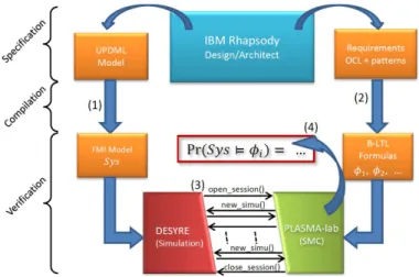
The interest of SMC [47, 42] is to propose an alternative to the approach of the classical model check-ing [5, 11]. By uscheck-ing results from the statistic area (includcheck-ing sequential hypothesis testcheck-ing or Monte Carlo simulation) in order to decide whether the system satisfies the property or not with some degree of confidence, SMC avoids an exhaustive exploration of the state-space of the model that generally does not scale up. It has already successfully experimented in biology area [10, 29, 39], software engineering [9] as well as industrial area[6] More recently, in DANSE[13], we adapt the SMC techniques to treat large heterogeneous systems like Systems of Systems. Among them, one finds systems integrating multiple heterogeneous distributed applications communicating over a shared network. We proposed to extend UPDM specification - the SoS specification - with some requirements that the SoS must satisfy. These requirements, are specified with the contract language we specially designed for the SoS’s. These goals are viewed as behavioral objectives that support the SoS architect in assessing different strategies and finding the best ones. As shown in Figure 2, these contracts are compiled into B-LTL formulas that are verified against the SoS (whose constituent systems are compiled into FMI executables) using the Statistical Model Checker Plasma-Lab [24] combined with the efficient simulation engine DESYRE de-veloped by Ales [2]. The SMC tool-chain gives an estimation of the satisfiability of the contract by the SoS. The different results help the SoS architect to make good decisions about how to optimize the SoS strategies.
Figure 2: The SMC process in DANSE
The main algorithm we used in DANSEis the Monte Carlo algorithm. This algorithm estimates the probability that a system Sys satisfies a B-LTL property P by checking P against a set of N random executions ofSyS. The estimation ˆpis given by
ˆ p=∑
N 1 f(exi)
N where f(exi) =1 ifexi|=P, 0 otherwise
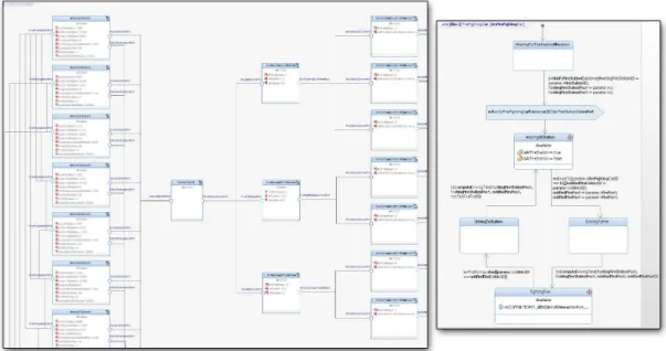
Figure 3: CAE incubator - architecture example and behavior of a fireman
also the capabilities to drive an external engine to perform the simulations like MathLab, SciLab, or DESYRE.
6
Illustration using the CAE incubator
In the frame of the DANSEproject, the Concept Alignment Example (CAE) is a fictive SoS example inspired by real-world Emergency Response data to a city fire. It has been built as a playground to demonstrate new methods and models for the analysis and visualization of SoS designs. All structural modeling has been performed using UPDM views, and behaviors have been added on a subset of the constituents that we called ”CAE incubator”, using simple SysML constructs (modeled in state machines) extended by a few stereotypes (e.g. for storing stochastic information).
Behavioral modeling in the CAE incubator is focused on following constituent systems: Fire HQ, Fire Station, Fire Fighting Car and District. The city districts have been added as constituent systems because they play an important role in the SoS: their behavior describes how the fires arise, expand and spread to neighbor districts. In the frame of the CAE, all behaviors are abstracted in state machines using IBM Rhapsody, but it would be possible to use any other language and tool as long as it is compliant with the FMI export format.
The following figure shows the overall architecture of the CAE incubator as well as the behavior of one of the constituent types: a fire fighting car.
We attached to the CAE incubator the following requirement, written accordingly to our proposed formalism:
”The mean city area under fire shall be less than 0.01%” mean(SoS.itsDistricts.fireArea→sum())≤0.01 %
specifi-cation for the statistical model checker Plasma-Lab and use it in conjunction with the simulation platform DESYRE to assess the probability that this goal is met in the specified time range (the simulation time for each run was 4 months). By choosing the Monte Carlo option, Plasma-Lab was able to give us the following estimation as a result on a given number of runs:
Prob(mean city area under fire≤0.01%)≈92.3%
In addition to the computation of the estimated probability that this goal is met on a given number of runs, Plasma-Lab can also compute how many runs are necessary to prove that a given probability threshold is passed by choosing the Chernov option.
Conclusion
This papers presents the results of the very first contract-based language for UPDM/SysML model of SoS we developed in the DANSEproject. The SoS model used in the project remains rather simple, but powerful enough to capture behaviors and requirements of a CAE case study developed in collaboration with EADS. Also, we are the first to study the relation between a modeling language used in industry (UPDM) and a verification approach developed by academic.
As a future work, we plan to offer more dynamicity, which we will do by exploiting and extending the work done on adaptative systems [48, 20, 8, 19]. This will also requires to adapt the UPDM framework. Another interesting future work will be to add more quantitative information directly in the patterns assumption and guarantee. This will permit us to reason on complex problematic such as energy con-sumption.
All these future extensions will be discussed and designed jointly with the business units as the DANSEpartners.
References
[1] The Open Group Architecture Forum. Available athttp://www.opengroup.org/togaf/.
[2] ALES:ALES S.r.l. - Advanced Laboratory on Embedded Systems. Available athttp://www.ales.eu.com/
site/.
[3] Alexandre ARNOLD, Benoˆıt BOYER & Axel LEGAY (2013): Contracts and Behavioral Patterns for SoS:
The EU IP DANSE approach.
[4] Modelica Association:Modelica. Available athttps://www.modelica.org/.
[5] Christel Baier & Joost-Pieter Katoen (2008): Principles of Model Checking (Representation and Mind
Se-ries). The MIT Press. Available athttp://mitpress.mit.edu/books/principles-model-checking.
[6] Ananda Basu, Saddek Bensalem, Marius Bozga, Benoît Delahaye & Axel Legay (2012):Statistical
abstraction and model-checking of large heterogeneous systems. Int. J. Softw. Tools Technol. Transf.14(1),
pp. 53–72, doi:10.1007/s10009-011-0201-2.
[7] Manfred Broy, Christian Leuxner & Tony Hoare, editors (2011): Software and Systems Safety -
Specifica-tion and VerificaSpecifica-tion. NATO Science for Peace and Security Series - D: Information and Communication
Security30, IOS Press.
[8] Cheng & all (2009): Software Engineering for Self-Adaptive Systems: A Research Roadmap. In: Software Engineering for Self-Adaptive Systems,LNCS5525, doi:10.1007/978-3-642-02161-9.
[9] Edmund Clarke, Alexandre Donz´e & Axel Legay (2010):On simulation-based probabilistic model checking
[10] Edmund M. Clarke, James R. Faeder, Christopher J. Langmead, Leonard A. Harris, Sumit Kumar Jha & Axel Legay (2008):Statistical Model Checking in BioLab: Applications to the Automated Analysis of T-Cell
Receptor Signaling Pathway. In Monika Heiner & AdelindeM. Uhrmacher, editors:Computational Methods
in Systems Biology,Lecture Notes in Computer Science5307, Springer Berlin Heidelberg, pp. 231–250, doi:10.1007/978-3-540-88562-7 18.
[11] Edmund M. Clarke, Jr., Orna Grumberg & Doron A. Peled (1999):Model checking. The MIT Press, Cam-bridge, MA, USA. Available athttp://mitpress.mit.edu/books/model-checking.
[12] M. D’Angelo, A. Ferrari, O. Ogaard, C. Pinello & A. Ulisse (2012): A Simulator based on QEMU and
SystemC for Robustness Testing of a Networked Linux-based Fire Detection and Alarm System. In:Online
proceedings of ERTS2 2012 - Embedded Real Time Systems and Software. Available at http://www.
erts2012.org/Site/0P2RUC89/4B-3.pdf.
[13] DANSE(2013):Designing for Adaptability and evolutioN in SoS Engineering. Available athttps://www.
danse-ip.eu/home/.
[14] DARPA:DARPA META Program. Available athttp://cps-vo.org/group/avm/meta/.
[15] UK Ministry of Defence: MODAF – Ministry of Defence Architecture Framework. Available at http:
//www.modaf.org.uk.
[16] USA Department of Defence: DoDAF – Department of Defence Architecture Framework. Available at
http://dodcio.defense.gov/dodaf20.aspx.
[17] A. Ferrari, M. Carloni, A. Mignogna, F. Menichelli, D. Ginsberg, E. Scholte & D. Nguyen (2012):Scalable
virtual prototyping of distributed embedded control in a modern elevator system. In: Industrial Embedded
Systems (SIES), 2012 7th IEEE International Symposium on, pp. 267–270, doi:10.1109/SIES.2012.6356593.
[18] A. Ferrari, L. Mangeruca, O. Ferrante & M. Mignogna (2012):DesyreML: a SysML profile for heterogeneous
embedded systems. In: Online proceedings of ERTS22012 - Embedded Real Time Systems and Software.
Available athttp://www.erts2012.org/Site/0P2RUC89/5B-1.pdf.
[19] Jasmin Fisher, Thomas A. Henzinger, Dejan Nickovic, Nir Piterman, Anmol V. Singh & Moshe Y. Vardi (2011):Dynamic Reactive Modules. In:CONCUR,LNCS6901, doi:10.1007/978-3-642-23217-6 27. [20] Carlo Ghezzi (2011):Engineering Evolving and Self-Adaptive Systems: An Overview. In Broy et al. [7], pp.
88–102, doi:10.3233/978-1-60750-711-6-88.
[21] IBM:IBM Rational Rhapsody Designer for Systems Engineering. Available athttp://www-142.ibm.com/
software/products/it/it/ratirhapdesiforsystengi/.
[22] Accellera Systems Initiative:Accelera Systems Initiative. Available athttp://www.accellera.org/. [23] INRIA:INRIA website. Available athttp://www.inria.fr/.
[24] INRIA (2012): Plasma-Lab: a Statistical Model Checker. Available at http://project.inria.fr/
plasma-lab/.
[25] IP-XACT: IP-XACT Technical Committee. Available at http://www.accellera.org/activities/
committees/ip-xact/.
[26] ITEA2: ITEA2 – Information Technology for European Advancement. Available athttp://www.itea2.
org/.
[27] ITEA2:Modelisar. Available athttp://www.itea2.org/project/index/view/?project=217. [28] Cyrille J´egourel, Axel Legay & Sean Sedwards (2012):A Platform for High Performance Statistical Model
Checking - PLASMA. In:TACAS, pp. 498–503, doi:10.1007/978-3-642-28756-5 37.
[29] Sumit K. Jha, Edmund M. Clarke, Christopher J. Langmead, Axel Legay, Andr´e Platzer & Paolo Zuliani (2009):A Bayesian Approach to Model Checking Biological Systems. In:Proceedings of the 7th International Conference on Computational Methods in Systems Biology, CMSB ’09, Springer-Verlag, Berlin, Heidelberg, pp. 218–234, doi:10.1007/978-3-642-03845-7 15.
[31] Mark W. Maier (1998):Architecting principles for systems-of-systems. Systems Engineering1(4), pp. 267– 284, doi:10.1002/(SICI)1520-6858(1998)1:4¡267::AID-SYS3¿3.0.CO;2-D.
[32] Mathworks:The Mathworks. Available athttp://www.mathworks.it/.
[33] MBAT:MBAT – combined Model-Based Analysis and Testing of embedded systems. Available athttps:
//www.mbat-artemis.eu/.
[34] OMG:Object Managment Group. Available athttp://www.omg.org/.
[35] OMG (2010):OCL v2.2 - Object Constraint Language. Available athttp://www.omg.org/spec/OCL/2. 2/.
[36] OMG (2011):UML v2.1.2. Available athttp://www.omg.org/spec/UML/2.1.2/.
[37] OMG (2012): UPDM – Unified Profile for DoDAF and MODAF. Available athttp://www.omg.org/
spec/UPDM/.
[38] Atos Origin (2011): MDT OCL/Ocl Checker. Available athttp://wiki.eclipse.org/MDT_OCL/Ocl_
Checker.
[39] Kwiatkowska M. Parker D., Norman G. (2012):The probabilistic model checker PRISM. Available athttp:
//www.prismmodelchecker.org.
[40] Modelica Association Project (2012):FMI v2.0 beta 4. Available athttps://www.fmi-standard.org/. [41] SysML Open Source Specification Project: SysML v. 1.3 Specification. Available athttp://www.sysml.
org.
[42] Koushik Sen, Mahesh Viswanathan & Gul Agha (2005): On Statistical Model Checking of Stochastic Sys-tems. In Kousha Etessami & Sriram K. Rajamani, editors:CAV, pp. 266–280, doi:10.1007/11513988 26.
[43] SPEEDS (2008): D 2.5.4: Contract Specification Language. Available at http://speeds.eu.com/
downloads/D_2_5_4_RE_Contract_Specification_Language.pdf.
[44] SPEEDS (2010):SPEculative and Exploratory Design in Systems Engineering. Available athttp://www.
speeds.eu.com/.
[45] SPRINT: SPRINT – Software PlatfoRm for Integration of eNgineering and Things. Available at http:
//www.sprint-iot.eu/.
[46] S Xiaoxia & Z Qiuhai (2003):MPII-18-3 The Introduction on High Level Architecture (HLA) and Run-Time
Infrastructure (RTI). In:SICE-ANNUAL CONFERENCE-, 1, SICE; 1999, pp. 1136–1139.
[47] Samir Younes, Edmund M. Clarke, Geoffrey J. Gordon & Jeff G. Schneider (2005): Verification and
Plan-ning for Stochastic Processes with Asynchronous Events. Technical Report, Carnegie Mellon University,
doi:10.1.1.68.4454.
A
Grammar
hcontracti ::= hviewpoint-idi+ ‘contract’hidentifieri {‘Assumption:’hpropertyi}? ‘Goal:’hpropertyi
‘Confidence:’hthresholdi
hviewpoint-idi::= ‘dynamicity’|‘behavior’|‘structure’|‘safety’|‘liveness’|. . .
hthresholdi ::= Float‘%’| hprobabilityi
hprobabilityi::= x, x∈(0; 1]
hpropertyi ::= hOCL-colli‘->forAll(’hvariablei‘|’hpatterni‘)’
| hOCL-colli‘->exists(’hvariablei‘|’hpatterni‘)’
| hOCL-propi | hpatterni
hpatterni ::= ‘whenever’ ‘[’hpropi‘]’ ‘occurs’ ‘[’hpropi‘]’ ‘holds’ ‘during’ ‘following’ ‘[’hinti‘]’
| ‘whenever’ ‘[’hpropi‘]’ ‘occurs’ ‘[’hpropi‘]’ ‘implies’ ‘[’hpropi‘]’ ‘during’ ‘following’ ‘[’hinti‘]’
| ‘whenever’ ‘[’hpropi‘]’ ‘occurs’ ‘[’hpropi‘]’ ‘does’ ‘not’ ‘occur’ ‘during’ ‘following’ ‘[’hinti‘]’
| ‘whenever’ ‘[’hpropi‘]’ ‘occurs’ ‘[’hpropi‘]’ ‘occurs’ ‘within’ ‘[’hinti‘]’
| ‘[’hpropi‘]’ ‘during’ ‘[’hinti‘]’ raises ‘[’hpropi‘]’
| ‘[’hpropi‘]’ ‘occurs’ ‘[’N‘]’ times during ‘[’hinti‘]’ ‘raises’ ‘[’hpropi‘]’
| ‘[’hpropi‘]’ ‘occurs’ ‘at’ ‘most’ ‘[’N‘]’ ‘times’ ‘during’ ‘[’hinti‘]’
| ‘[’hpropi‘]’ ‘during’ ‘[’hinti‘]’ ‘implies’ ‘[’hpropi‘]’ ‘during’ ‘[’hinti‘]’ ‘then’ ‘[’hpropi‘]’ ‘during’ ‘[’hinti‘]’
hpropi ::= hOCL-propi | harith-reli
harith-reli ::= hexpri( ‘<’|‘<=’|‘=’|‘>=’|‘>’ )hexpri
harith-expri ::= hexpri hoperatori hexpri |‘(’hexpri‘)’
| hOCL-expri
| ‘mean(’hOCL-expri‘)’|‘sum(’hOCL-expri‘)’
| ‘prod(’hOCL-expri‘)’|‘at(’hOCL-expri‘,’htimei‘)’
hoperatori ::= ‘+’|‘-’|‘*’|‘/’
htimei ::= Nhtime-uniti |+∞
htime-uniti ::= ‘ms’|‘s’|‘min’|‘hour’|‘day’|. . .
The non-terminalhtime-unitican be any multiple of the application basic time unit ( i.e. day, hour, min, sec, ms, ...). The latest revision of the OCL specification can be found at [35] and more particularly the grammar of the language. We just give an overview of the relevant subset used in this language:
hOCL-propositioni stands for the simple Boolean expressions over collections or primitive types (int, real, boolean, . . . ) of OCL. We also identifiedhOCL-expri, the OCL subset of non-Boolean expression, e.g. Component Collections (without treatments, e.g. the functionsmap(...), iter(...) ), numeri-cal values, model-related values, . . . Some relevant details about OCL collections are in the chapters 7.7 (Collection operations) and 11.6 (Collection-related types) of the OCL specification [35].
B
Patterns
We give the list of all the SPPEDS patterns we reuse and we give give their semantics based on the statifiability given in Section 3.
a. wheneverΨ1occursΨ2holds during following[a,b]
The interval[a,b]is located relatively after the satisfaction ofΨ1. The interval, in whichΨ2must be satisfied, startsaunits of time after the observed occurrence ofΨ1.
b. Ψ1impliesΨ2holds forever
From the very moment whenΨ1is satisfiedΨ2must hold during all the rest of the execution path.
c. alwaysΨ
Ψmust hold during all the execution path.
d. wheneverΨ1occursΨ2holds
As for the previous pattern, the interval [a,b]is relative. At each time value between aand b. whereΨ1holds,Ψ2must also hold. ReplacingΨis replaced bytrueallows to create a new sim-pler pattern:
Ψ1impliesΨ2during following[a,b]
f. wheneverΨ1occursΨ2does not occur during following[a,b]
This pattern specifies thatΨ2 is never satisfied during the relative interval[a,b], i.e. ¬Ψ2 holds during[a,b].
g. wheneverΨ1occursΨ2occurs within[a,b]
The constraintΨ2must be satisfied at less one time during[a,b]afterΨ1.
h. Ψ1occursntimes during[a,b]raisesΨ2
WhenΨ2is satisfied at lessntimes during[a,b],Ψ2starts to hold atb.
i. Ψoccurs at mostntimes during[a,b]
As previously mentioned, an occurrence ofΨis counted whenΨbecomes satisfied. If Ψholds for a state in[a,b], to observeΨholds for the following one (also in[a,b]) does not increase the occurrence number ofΨ.
IfΨ1holds during[a,b]thenΨ2must hold atb.
k. Ψduring[a,b]impliesΨ1during[a,c]thenΨ2during[c,b]
WheneverΨholds during[a,b]there exists a split atcof[a,b]such thatΨ1holds during[a,c]then