VISIR-I: small vessels, least-time nautical routes using wave forecasts

(1)

GMDD

8, 7911–7981, 2015

VISIR-I: least-time nautical routes

G. Mannarini et al.

Title Page

Abstract Introduction

Conclusions References

Tables Figures

◭ ◮

Back Close

Full Screen / Esc

Printer-friendly Version Interactive Discussion

Discussion

P

a

per

|

Discussion

P

a

per

|

Discussion

P

a

per

|

Discussion

P

a

per

|

Geosci. Model Dev. Discuss., 8, 7911–7981, 2015 www.geosci-model-dev-discuss.net/8/7911/2015/ doi:10.5194/gmdd-8-7911-2015

This discussion paper is/has been under review for the journal Geoscientific Model Development (GMD). Please refer to the corresponding final paper in GMD if available.

VISIR-I: small vessels, least-time nautical

routes using wave forecasts

G. Mannarini1, N. Pinardi1,2,3, G. Coppini1, P. Oddo2,a, and A. Iafrati4

1

Centro Euro–Mediterraneo sui Cambiamenti Climatici – Ocean Predictions and Applications, via Augusto Imperatore 16, 73100 Lecce, Italy

2

Istituto Nazionale di Geofisica e Vulcanologia, Via Donato Creti 12, 40100 Bologna, Italy

3

Università degli Studi di Bologna, viale Berti-Pichat, 40126 Bologna, Italy

4

CNR-INSEAN, Via di Vallerano 139, 00128 Roma, Italy

a

presently at: NATO Science and Technology Organisation – Centre for Maritime Research and Experimentation, Viale San Bartolomeo 400, 19126 La Spezia, Italy

Received: 1 August 2015 – Accepted: 14 August 2015 – Published: 11 September 2015

Correspondence to: G. Mannarini ([email protected])

(2)

GMDD

8, 7911–7981, 2015

G. Mannarini et al.

Title Page

Tables Figures

◭ ◮

Back Close

Full Screen / Esc

Discussion

P

a

per

|

Discussion

P

a

per

|

Discussion

P

a

per

|

Discussion

P

a

per

|

Abstract

A new numerical model for the on-demand computation of optimal ship routes based on sea-state forecasts has been developed. The model, named VISIR (discoVerIng Safe and eﬀ_{Icient Routes) is designed to support decision-makers when planning a marine}

voyage.

5

The first version of the system, VISIR-I, considers medium and small motor vessels with lengths of up to a few tens of meters and a displacement hull. The model is made up of three components: the route optimization algorithm, the mechanical model of the ship, and the environmental fields. The optimization algorithm is based on a graph-search method with time-dependent edge weights. The algorithm is also able to

com-10

pute a voluntary ship speed reduction. The ship model accounts for calm water and added wave resistance by making use of just the principal particulars of the vessel as input parameters. The system also checks the optimal route for parametric roll, pure loss of stability, and surfriding/broaching-to hazard conditions. Significant wave height, wave spectrum peak period, and wave direction forecast fields are employed as an

15

input.

Examples of VISIR-I routes in the Mediterranean Sea are provided. The optimal route may be longer in terms of miles sailed and yet it is faster and safer than the geodetic route between the same departure and arrival locations. Route diversions result from the safety constraints and the fact that the algorithm takes into account the full temporal

20

evolution and spatial variability of the environmental fields.

1 Introduction

The operational availability of high spatial and temporal resolution forecasts, for both weather, sea-state and oceanographic variables opens the way to a realm of downstream services, which are increasingly closer to end-user needs (Proctor and

25

Howarth, 2008). Such services may support the decisional process in critical situations

(3)

GMDD

8, 7911–7981, 2015

G. Mannarini et al.

Title Page

Tables Figures

◭ ◮

Back Close

Full Screen / Esc

Discussion

P

a

per

|

Discussion

P

a

per

|

Discussion

P

a

per

|

Discussion

P

a

per

|

where knowledge of the present and predicted environmental state is key to avoiding casualties or to making savings in terms of time, cost, or environmental impact.

VISIR [vi’zi:r]1is a model and an operational system2for the on-demand computation of safe and eﬃ_{cient ship routes, based on sea-state forecasts. In its present version,}

VISIR-I, medium and small motor vessels with displacement hulls are considered, such

5

as: fishing vessels (e.g. seiners, trawlers), towboats and fireboats, service boats (crew and supply boats), short trip coastal freighters, displacement hull yachts and pleasure crafts, and small ferry boats.

The aim of this paper is to lay a sound scientific foundation of VISIR-I, including all its main components: the optimization algorithm, the ship model, and the processing

10

of the environmental fields.

After reviewing the literature in Sect. 1.1 and summarizing our original contribution in Sect. 1.2, the solution devised for VISIR-I is presented in detail in Sect. 2. Examples of optimal routes in the Mediterranean Sea, (Sect. 3), precede the conclusions, which are drawn in Sect. 4.

15

1.1 Review of literature

The main mathematical schemes available in the literature to solve ship routing prob-lems are reviewed in the following.

Initially devised as a manual tool for navigators, the isochrone method is based on the idea of building an envelope of positions attainable by a vessel at a given time lag

20

after departure. This envelope is called an “isochrone”. In the work by Hagiwara (1989), a detailed algorithm is provided, describing how to generate the isochrones and how to use them for constructing a least-time route. Space and course discretization in the vicinity of the rhumb line between departure and arrival locations are performed. At

1

“Visir” is the Italian for “vizier”, who was a high-ranking political advisor in the Arab world. Its etymology seems to be related to the ideas of “deciding” and “supporting”.

2

(4)

GMDD

8, 7911–7981, 2015

G. Mannarini et al.

Title Page

Tables Figures

◭ ◮

Back Close

Full Screen / Esc

Discussion

P

a

per

|

Discussion

P

a

per

|

Discussion

P

a

per

|

Discussion

P

a

per

|

each progress stage, the course leading to the maximum spatial advancement from the origin is considered. When an isochrone gets close enough to the destination, the optimal route is recovered by a backtracking procedure. No proof of the time-optimality of the resulting route is provided. Hagiwara’s modified isochrone method is the ba-sis for the fuel optimization method proposed by Klompstra et al. (1992). Here, each

5

stage is represented by a two-dimensional position and time. Instead of isochrones or time-fronts, energy-fronts or “isopones” are computed, being the attainable regions for a given expenditure on fuel. Szlapczynska and Smierzchalski (2007) review several variants of the isochrone method, highlighting their weaknesses, such as limitations in the form of ship speed characteristics and in dealing with landmasses, especially

10

in the vicinity of narrow straits. The authors propose a solution to the latter issue, by screening all route portions intersecting the landmass.

The variational approach involves searching for trajectories making an objective func-tional stationary, such as total time of navigation or operafunc-tional cost, given a set of constraints. The search is achieved by varying the parameters controlling the

trajec-15

tory. This approach is equivalent to solving the Euler–Lagrange equation. In Hamilton (1962), least-time ship routes are computed by varying the ship’s course, under the as-sumption that the environmental field is static and thus vessel speed does not explicitly depend on time.

The time-dependent problem instead can be addressed through the technique of

20

optimal control (Pontriagin et al., 1962). With this method, the dynamic system (the vessel) is controlled by a time-dependent input function (typically engine thrust and rudder angle), allowing the objective function to be minimized. Optimal control is for-mulated in terms of a set of necessary conditions (Luenberger, 1979). Applications of optimal control to ship routing problems are found in Bijlsma (1975), Perakis and

25

Papadakis (1989) and Techy (2011). Least-time transatlantic routes are computed by Bijlsma (1975). There, significant wave height and wave direction fields from 12 hourly forecasts are assumed to determine vessel speed, while the sole control variable is vessel course. The method can account for prohibited courses due to dynamic

(5)

GMDD

8, 7911–7981, 2015

G. Mannarini et al.

Title Page

Tables Figures

◭ ◮

Back Close

Full Screen / Esc

Discussion

P

a

per

|

Discussion

P

a

per

|

Discussion

P

a

per

|

Discussion

P

a

per

|

sons (e.g. rolling). However, specific geometrical conditions on the vessel speed char-acteristics have to hold for the method to work. Furthermore, due to topological issues, there are unreachable regions of the ocean, and the method involves guessing the initial vessel course, which may hinder the implementation in an automated system. The approach by Perakis and Papadakis (1989) accounts for a delayed departure time

5

and for passage through an intermediate location (point-constrained problem). Local optimality conditions (“broken extremals”) are found at the boundaries of spatial sub-domains. The optimal ship power setting is found to always take the maximum value possible. The results hold under the assumption that the ship speed characteristics depend on engine throttle as a multiplicative factor. Another limitation of this approach

10

is that the computed extremal trajectory is not guaranteed to lead to a minimum of the objective function (instead a maximum could be retrieved). In Techy (2011) the author reports on a vessel moving with constant velocity with respect to water in presence of currents (“Zermelo’s problem”). The optimal trajectory is analyzed as a function of flow divergence and vorticity, finding the optimal steering policy in a point-symmetric,

15

time-varying flow field. In addition, a geometrical interpretation of Pontriagin’s principle is provided. However, to deliver a unique solution, the method requires the hypothesis that the domain of maneuverability of the ship is convex.

The work by Lolla et al. (2014) is based on the computation of the reachability front of a vehicle with an internal propulsion system, subject to a time-dependent ocean flow.

20

The front is implicitly defined through a level set, and its evolution satisfies a specific solution of a Hamilton–Jacobi equation. The optimal speed of the vehicle is found to always take the maximum value admissible. The actual trajectory is computed via back-tracking. This approach allows for both stationary and mobile obstacles, and is able to compute an optimal departure time for the vehicle. The use of generalized gradients

25

and co-states overcome the hypothesis of regularities of the level set. This promising method is at present still lacking an operational implementation.

(6)

GMDD

8, 7911–7981, 2015

G. Mannarini et al.

Title Page

Tables Figures

◭ ◮

Back Close

Full Screen / Esc

Discussion

P

a

per

|

Discussion

P

a

per

|

Discussion

P

a

per

|

Discussion

P

a

per

|

Monte Carlo methods makes use of genetic algorithms. They start with guessed routes (“chromosomes”) whose subparts (“genes”) cross each other and mutate in a random way, in order to find a new route (“oﬀ_{spring”) that better fits the objective function of}

the actual problem. The use of Monte Carlo methods in the context of multi-objective optimization is reviewed in Konak et al. (2006), while an application to ship routing

5

is provided by Szlapczynska (2007). There is also a simulated annealing approach to ship routing (Kosmas and Vlachos, 2012). In this case, in order to find a global optimum a trial route is perturbed in a statistical-mechanical fashion. Given that in Monte Carlo methods there is no exact analytical solution, additional criteria are needed in order to decide whether a solution is satisfactory (“convergence test”).

10

In discrete methods, the spatial domain is represented by some kind of grid (regu-lar or not) and the optimization is based on recursive schemes. A key concept is the so called principle of optimality: given a point on the optimal trajectory, the remaining trajectory is optimal for the minimization problem initiated at that point (Luenberger, 1979). This property can be stated as a recursive relation, called “Bellman’s

condi-15

tion” in the framework of discrete methods. In Zoppoli (1972) a dynamic programming method for the computation of a least-time ship route in the Indian Ocean is used. The algorithm is able to ingest time-dependent environmental fields, by evaluating them at the nearest quantized time value. However, the actual case-study provided in the paper just uses stationary fields. Ship operating costs for transatlantic routes are minimized

20

in Chen (1978), where a terminal cost is also included in the objective function. The grid used however is just a band of gridpoints along the rhumb-line track, thus being limited in terms of application when there are complex topological constraints, such as in a coastal environment. Takashima et al. (2009) use dynamic programming for com-puting minimum fuel routes of a given duration in time. The propeller revolution number

25

is kept constant during the voyage and its value is adjusted in order to reach the target route duration. The ship course is varied in order to exploit ocean currents. However, the algorithm uses static environmental information, and re-routing is run every three hours in order to deal with dynamic currents. The dynamic programming method by

(7)

GMDD

8, 7911–7981, 2015

G. Mannarini et al.

Title Page

Tables Figures

◭ ◮

Back Close

Full Screen / Esc

Discussion

P

a

per

|

Discussion

P

a

per

|

Discussion

P

a

per

|

Discussion

P

a

per

|

Wei and Zou (2012) is used to minimize fuel consumption. Both throttle and heading of the vessel can be optimized, again with grid limitations as in Chen (1978). Montes (2005) employs Dijkstra’s algorithm to compute least-time routes in time-varying fore-cast fields. However, the eﬀ_{ect of weather on vessel speed is parametrized in terms of}

subjective parameters (“speed penalty function”).

5

1.2 Our contribution

There are several recurrent shortcomings in the ship routing literature: the limited ca-pability to deal with complex topological conditions, such as in the coastal environment (Bijlsma, 1975; Hagiwara, 1989; Szlapczynska and Smierzchalski, 2007); the need for heuristics or subjective parameters in the optimization algorithm (Kosmas and Vlachos,

10

2012; Montes, 2005); non explicit use of time-dependent environmental information (Hamilton, 1962; Zoppoli, 1972; Takashima et al., 2009); limitations on the functional dependence of the vessel response function (Perakis and Papadakis, 1989; Techy, 2011); and the not yet demonstrated use in an operational environment (Lolla et al., 2014).

15

All these issues need to be addressed simultaneously by a model aimed at feeding an operational system that also works in coastal waters, for a wide class of vessels and environmental conditions, taking into account navigation safety according to the latest international standards. In VISIR-I all the above mentioned shortcomings are overcome. The method is based on an exact graph search algorithm, modified in order

20

to manage time-dependent environmental fields and voluntary vessel speed reduction. It is validated against analytical results. In addition, the graph grid is designed to deal with the topological requirements of coastal navigation. VISIR-I also includes a dedi-cated motorboat model and safety constraints for vessel intact stability are considered.

All these features are described in detail in what follows.

(8)

GMDD

8, 7911–7981, 2015

G. Mannarini et al.

Title Page

Tables Figures

◭ ◮

Back Close

Full Screen / Esc

Discussion

P

a

per

|

Discussion

P

a

per

|

Discussion

P

a

per

|

Discussion

P

a

per

|

2 VISIR-I method

In this section we present the method employed by VISIR-I for solving the route op-timization problem. First, the problem is formally stated (Sect. 2.1), then the solution algorithm (Sect. 2.2), the mechanical model of the ship (Sect. 2.3) and the processing of the environmental analysis and forecast fields aﬀ_{ecting the ship dynamics (Sect. 2.4)} 5

are presented. The structure of the computer code is provided in Sect. 2.5 and a vali-dation of the resulting optimal routes is given in Sect. 2.6.

2.1 Statement of the problem

The mathematical problem addressed and solved in an operational way by VISIR-I can be stated as follows.

10

A ship route is sought departing fromA=₍_x_A_,_t_A_{) and arriving at}_B=₍_x_B_,t_A+_{J) and}

minimizing the sailing timeJ defined by

J= 1

c B Z

A

n(x,t) ds (1)

wherex=_[x(t),_y_(t)]T _{within an open set}Ω_⊂_R2 _{denotes horizontal position,}_t _{is the}

time variable, and

15

n(x,t)=_c/v(_x_{,t) ,} ₍₂₎

with vessel speedcin calm weather conditions and sustained speedv(x,t) in specific meteo-marine conditions, is the “refractive index” of a horizontal domain of linear extent dssuch that

ds2=_dx2+_dy2 ₍₃₎

20

Note that the integrand in Eq. (1) can be interpreted as an eﬀ_{ective optical depth of}

(9)

GMDD

8, 7911–7981, 2015

G. Mannarini et al.

Title Page

Tables Figures

◭ ◮

Back Close

Full Screen / Esc

Discussion

P

a

per

|

Discussion

P

a

per

|

Discussion

P

a

per

|

Discussion

P

a

per

|

of light moving in a non homogenous medium. Indeed light propagates over paths of stationary optical depth (Fermat’s principle).

Ship speed v results from a dynamic balance between forces and torques acting on and from the vessel. This speed is normally found as the solution of diﬀ_erential

equations. However, under steady conditions they reduce to algebraic equations of the

5

type:

Feq(v;ps,pe)=0 (4)

wherep_s is a set of ship parameters andp_ea set of values of relevant environmental fields evaluated at (x,t). Navigational safety also poses limitations on the admissible solutions of Eq. (4). Such limitations are represented as a set of inequalities of the type:

10

Fineq(v;ps,pe)≤0 (5)

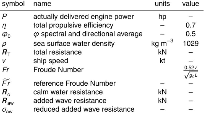
Parametersp_sandp_eemployed in Eqs. (4) and (5) are listed in Table 6.

If the open set Ω _{is also a connected domain, the existence of a solution to the}

problem Eqs. (1)–(5) entirely depends on Eqs. (4) and (5): The quality of the route, its topological and nautical characteristics, are determined by these two equations alone.

15

Speed v resulting from Eqs. (4) and (5) defines the Lagrangian kinematics of the route:

ds

dt =v(x,t) (6)

In order to account for uncertainty in the representation ofv, a random noise term could be added to the r.h.s. of Eq. (6).

20

The problem of finding the least-time route in any meteo-marine conditions is thus equivalent to the minimization ofJ functional with a specified refractive index n(x,t), for assigned boundary valuesAandB.

If the time-dependence in refractive indexnis neglected, the general solution of this problem is known from geometrical optics, with routes being refracted towards optically

(10)

GMDD

8, 7911–7981, 2015

G. Mannarini et al.

Title Page

Tables Figures

◭ ◮

Back Close

Full Screen / Esc

Discussion

P

a

per

|

Discussion

P

a

per

|

Discussion

P

a

per

|

Discussion

P

a

per

|

more transparent regions, according to Snell’s law. However, whenever the time scale for changes in the environmental fields is comparable or shorter than the typical route duration, such time-dependence can no longer be neglected and new kinematical fea-tures of the least-time route may appear. Indeed, it could be advantageous to wait for some time at the departure location before leaving or voluntarily decrease the speed

5

during navigation, as shown in Sect. 2.2.2 and 2.2.3.

2.2 Shortest path algorithm

The first component of VISIR-I presented here is the shortest path algorithm. The term “shortest path” is used both in the literature and hereafter with a more general sense than a direct reference to the geometrical distance. Indeed, “shortest” may refer to the

10

spatial or temporal distance, as well as the cost or other figure of merit of the optimal path.

2.2.1 Spatial discretization

Let us consider a directed graph_G=_[_N_,_E_{]. In VISIR-I the nodes}_N _{are part of a}

rect-angular mesh with constant spacing in natural coordinates (1/60◦of resolution in both

15

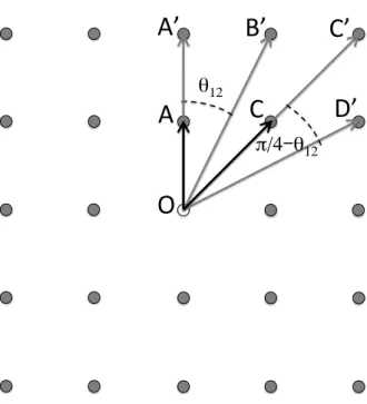
latitude and longitude). As shown in Fig. 1, each node is linked to all its first and second neighbours on the grid, forming the set of edges _E. Thus, neglecting border eﬀ_ects,

there are 24 connections per node. The specific edge arrangement leads to resolve angles of

θ12=arctan(1/2)≈26.6◦ (7)

20

Whether such such 24-connectivity should be increased further is questionable, given that the environmental analysis and forecast fields are provided on a coarser grid (by about a factor of 4) than the spatial resolution of the graph, see Sect. 2.4.

In VISIR-I, the resulting graph is first screened for nodes and edges on the landmass. An edge is considered to be on the landmass if at least one of its nodes is on the

25

(11)

GMDD

8, 7911–7981, 2015

G. Mannarini et al.

Title Page

Tables Figures

◭ ◮

Back Close

Full Screen / Esc

Discussion

P

a

per

|

Discussion

P

a

per

|

Discussion

P

a

per

|

Discussion

P

a

per

|

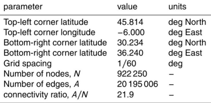
landmass or if both nodes are in the sea and the edge linking them intersects the coastline. In such a case, the edge is removed fromE, which locally reduces the original 24-connectivity of the graph. When applied to a 1/60◦ grid for the Mediterranean Sea region (mode 1 of Fig. 8), this procedure still leaves more than 20 million sea edges in E, see Table 2. However, for the actual route computations, just a subset of the whole

5

spatial domain is considered (mode 2 of Fig. 8). This subregion is chosen to be large enough so that a further increase in size does not reduce the total sailing timeJ. At present, the selection of the subregion shape and extent is left to the user of the model.

2.2.2 Time-dependent approach

Given that environmental conditions change over a time scale comparable with or

10

shorter than the vessel route duration, edge weights cannot be considered as con-stants. Thus, in order to solve Eqs. (1)–(3), VISIR-I employs a time-dependent algo-rithm.

With reference to the nomenclature in Table 1, a time-dependent graph _G(t) is fully defined by the sets of nodes, edges, and time-dependent edge weights: G(t)= 15

[_N,_E,_A(t)].

Edge weighta_{j k}(ℓ) between nodesj andk at time stepℓ is defined as

a_{j k}(ℓ)=|xk−xj|

vj k(ℓ)

(8)

wherevj k(ℓ) is the edge mean ship speed, depending on the averageΦj k of the values of the environmental fields at nodesj andk:

20

Φ_{j k}=1

2 Φj+ Φk

(9)

evaluated at timet_ℓ =_t₁+_δ_t_(ℓ₋_{1). Here}_t₁ _{is departure time and}_δ_t _{is the time}

reso-lution of the environmental fields. The functional dependence ofv_{j k}(ℓ) onΦ_{j k} _results

(12)

GMDD

8, 7911–7981, 2015

G. Mannarini et al.

Title Page

Tables Figures

◭ ◮

Back Close

Full Screen / Esc

Discussion

P

a

per

|

Discussion

P

a

per

|

Discussion

P

a

per

|

Discussion

P

a

per

|

Thus, in VISIR-I, edge weightsaj k(ℓ) are non-negative quantities with a dimension of time (“edge delays”) and are time-dependent. Note that Eq. (8) is the discrete coun-terpart of Eq. (6), as long as velocity is non null.

There are various methods for computing shortest paths on a graph. For an overview, see Bertsekas (1998) and Bast et al. (2014). A large literature deals with applications

5

for terrestrial networks, see e.g. Zhan and Noon (1998); Zeng and Church (2009); Goldberg and Harrelson (2005).

A key concept in graph methods is the node label, which can be either temporary or permanent. The permanent labelX_j of node j is the minimum value of the objective function (e.g. J of Eq. 1) attainable at that node. A temporary label Y_j is any value

10

before the node label is set to its permanent value. When all node labels are set to their permanent value, Bellman’s relation holds (Bertsekas, 1998).

Depending on the way node labels are updated, graph algorithms may be classified into label setting or label correcting algorithms. A label setting source single-destination algorithm with fixed departure time is used here.

15

The fact that in VISIR-I destination node is assigned (through x_B in Eq. 1) leads to a possible degeneracy of the problem, with multiple shortest paths between the specified source and destination node. In Yen (1971) an algorithm is presented for finding several simple shortest paths. In VISIR-I it is deemed that, in presence of time-dependent environmental fields, it is unlikely that an alternative route with exactly the

20

same navigation time exists. Thus, just the least-time route is sought after.

In general, the fact that a graph is time-dependent means that the shortest path can have special features. In fact, under specific circumstances, the strategy of traversing an edge as soon as possible does not always lead to the shortest path. Also, the short-est path may not be simple (there may be loops) or even not concatenated (Bellman’s

25

optimality not fulfilled). This has consequences on the class of algorithm to be applied. Orda and Rom (1990) show that in this respect the critical condition is how fast edge delays vary in time. Ifa_{j k}(t) is a diﬀ_{erentiable function of time}_{t, the authors show that,}

(13)

GMDD

8, 7911–7981, 2015

G. Mannarini et al.

Title Page

Tables Figures

◭ ◮

Back Close

Full Screen / Esc

Discussion

P

a

per

|

Discussion

P

a

per

|

Discussion

P

a

per

|

Discussion

P

a

per

|

provided d

dtaj k(t)≥ −1 , (10)

the best strategy for recovering a shortest path is traversing edge (jk) without waiting at nodej (First-In First-Out or: FIFO). Indeed, waiting for a time dt >0 would in best case be compensated but never overcome by a related decrease_|daj k| ≤dt in edge

5

delay. The authors also show that a FIFO time-dependent algorithm has the same computational complexity as a static algorithm.

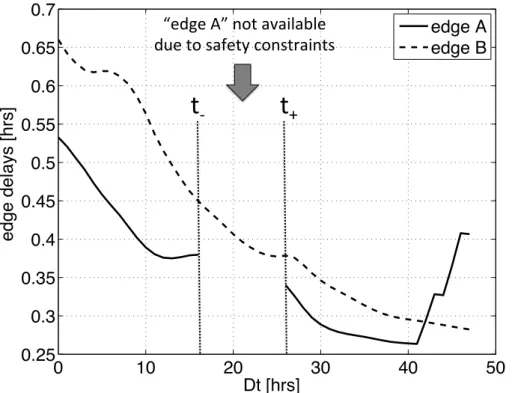
Typically, condition Eq. (10) may be violated during the decaying phase of a rapidly moving storm. Since VISIR-I employs sea state fields for the Mediterranean Sea, the variability of edge delays is usually low, so that condition Eq. (10) is generally fulfilled,

10

as seen from Fig. 2. The FIFO condition Eq. (10) is also checked at each run of the model and is generally found to be fulfilled. Thus, Dijkstra’s static algorithm (Dijkstra, 1959) is modified according to the guidelines of Orda and Rom’s FIFO time-dependent algorithm. Related pseudocode is provided in Appendix A.

Before the algorithm is run, edge delays aj k(ℓ) are checked for nautical safety

15

constraints, Eq. (5). If at time step ℓ an edge (j k) is unsafe for navigation, we set a_{j k}(ℓ)=_∞_{. As seen from Fig. 2, this approach generates gaps in}_a

j k(t) as a function of continuous time t. Such gaps are specific time windows during which the edge is not available for linking its nodes. Whenever edges are removed at specific time steps, a FIFO strategy is no longer guaranteed to be optimal, even though edge delays vary

20

slowly. A source-waiting strategy may be necessary in this case (Orda and Rom, 1990). As a consequence, a route retrieved through a FIFO algorithm may still be sub-optimal. This advanced issue is left open for future versions of the system.

2.2.3 Voluntary speed reduction

As seen above, VISIR-I’s strategy regarding navigational safety is to remove unsafe

25

(14)

GMDD

8, 7911–7981, 2015

G. Mannarini et al.

Title Page

Tables Figures

◭ ◮

Back Close

Full Screen / Esc

Discussion

P

a

per

|

Discussion

P

a

per

|

Discussion

P

a

per

|

Discussion

P

a

per

|

of the optimal route. In addition, as will be shown in Sect. 2.3.3, vessel speedv aﬀ_ects

the safety constraints. Thus, a modification ofv may help in keeping an otherwise un-safe edge in the graph. This, in turn, may contribute to optimization, since avoiding the removal of elements from set_A(t) can only lower the length of the shortest path. Such voluntary variations in speed should be contrasted with an involuntary speed

reduc-5

tion due to vessel energy loss, caused by interaction with the environmental fields, see Sect. 2.3.2.

VISIR-I defines, for a vessel with maximum engine power Pmax, a set of possible

valuesP(s)/P_maxof engine throttle:

P(s)₌_P

max·g(s) (11)

10

s_∈[1,Ns]

Then, at each edge, speedsv_{j k}(s)(ℓ) are computed using the ship model. The function g(s) is chosen in order to linearly space engine throttle values, Table 3 (due to the non-linearity of the vessel model, this choice does not imply linearly spaced values of sustained speed, see Fig. 5). Next, throttle-dependent edge weightsa(_{j k}s)(ℓ) are

com-15

puted via Eq. (8). Each of these edge weights is checked to see whether it complies with navigational safety constraints. If an edge is unsafe, its edge weight is set to∞. Finally, the throttle values∗leading to the minimum edge weight is chosen by the algo-rithm:

s∗=_argmin s

n

a(_{j k}s)(ℓ)o (12)

20

and the edge weight is set to such a minimum value:

a_{j k}(ℓ)=_a(s∗)

j k (ℓ) (13)

Given the ordering in Table 3, if s∗>1 then voluntary speed reduction is useful for recovering a faster route which is still safe with respect to ship stability constraints.

(15)

GMDD

8, 7911–7981, 2015

G. Mannarini et al.

Title Page

Tables Figures

◭ ◮

Back Close

Full Screen / Esc

Discussion

P

a

per

|

Discussion

P

a

per

|

Discussion

P

a

per

|

Discussion

P

a

per

|

2.3 Ship model

The second component of VISIR-I is a ship model describing vessel interaction with the environment (specified by the forecast fields of Sect. 2.4) and its stability requirements. The following presentation comprises a balance equation for the propulsion sys-tem Sect. 2.3.1, a parametrization of the hull resistance due to calm and rough sea

5

Sect. 2.3.2, and a set of dynamic conditions for the intact stability of the vessel Sect. 2.3.3.

2.3.1 Propulsion

Motorboats are the focus of VISIR-I route optimization.

For these vessels, propulsion is provided by a thermal engine burning fuel and

deliv-10

ering a torque to the shaft line and, when present, to a gearbox. This torque is eventu-ally transmitted to a propeller, converting it into thrust available to counteract resistance to advancement (Journée, 1976; Triantafyllou and Hover, 2003).

A full modelling of this energy conversion mechanism is a highly complex task involv-ing, just to mention a few, the eﬃ_{ciency of each of these conversion steps, the e}ﬀ_ect 15

of hull-generated wake on propeller eﬃ_{ciency and corresponding thrust deduction, and}

the load conditions of the engine (MANDieselTurbo, 2011). A quantitative description of these processes requires a detailed knowledge of engine and vessel behaviour. This could be obtained by standard measurement procedures such as those provided by the International Towing Tank Conference (ITTC, 2002, 2011b).

20

For the purposes of VISIR-I, it was deemed suﬃ_{cient to derive the vessel response}

function from a power balance. That is, given the brake powerP, the total propulsive eﬃ_ciency_η_{and the total resistance}_R_T _{applied to}_{the vessel, it is required that}

ηP =₋_v_·_R_T_(v₎ ₍₁₄₎

wherev is ship velocity in steady conditions. The l.h.s. of Eq. (14) represents the power

25

(16)

GMDD

8, 7911–7981, 2015

G. Mannarini et al.

Title Page

Tables Figures

◭ ◮

Back Close

Full Screen / Esc

Discussion

P

a

per

|

Discussion

P

a

per

|

Discussion

P

a

per

|

Discussion

P

a

per

|

ship parameters. One of its possible representations is derived in Sect. 2.3.2. The eﬃ_ciency_η_{results from the product of several components related, for example, to hull}

shape, propeller, and shaft characteristics (MANDieselTurbo, 2011). At the present stage of modelling, the value ofηis estimated to a constant (see Table 4) and will be refined when a more detailed vessel model is used.

5

2.3.2 Resistance

In this paper we restrict our attention to displacement vessels. Indeed high speed plan-ing hulls are characterized by a diﬀ_{erent dynamic behaviour and deserve a more}

so-phisticated treatment (Savitsky and Brown, 1976).

When underway, a displacement vessel is subject to various forces hindering its

10

motion. A possible decomposition of the resulting force is to distinguish calm water resistanceR_cfrom resistanceR_awdue to only sea waves,

R_T=_R_c+_R_aw ₍₁₅₎

Since calm water resistance is always opposite to the ship direction of advance, de-composition Eq. (15) enables Eq. (14) to be rewritten as

15

ηP =_v_(R_c+_R_aw_cos_α) ₍₁₆₎

whereα is the angle between wave direction and vessel direction of advance (as seen from Fig. 3,α=_{0 in case of head waves).}

The module of the calm water resistance is usually given in terms of a dimensionless drag coeﬃ_cient_C_T _{defined by the equation}

20

Rc(v)=CT

1 2ρSv

2

(17)

where also sea water densityρand ship wetted surfaceS appear.

(17)

GMDD

8, 7911–7981, 2015

G. Mannarini et al.

Title Page

Tables Figures

◭ ◮

Back Close

Full Screen / Esc

Discussion

P

a

per

|

Discussion

P

a

per

|

Discussion

P

a

per

|

Discussion

P

a

per

|

As outlined in ITTC (2011a),CT depends not just on viscous eﬀects but also on

en-ergy dissipated in gravity waves generated by the vessel (“residual resistance”). The latter introduces a dependence on Froude NumberFr which, under Froude’s hypoth-esis, is additive:CT(R,F r)≈CF(R)+CR(F r), whereR is Reynold’s number andCRis

the residual resistance drag coeﬃ_{cient (Newman, 1977).} 5

In VISIR-I, at this first stage in the development of the ship model, CT is taken as

a constant. This is done in order to easily identify the unknown coeﬃ_{cients in the r.h.s.}

of Eq. (17). Indeed, theCTS product is obtained by equating the maximum available

power at the propeller to the power dissipation occurring at top speedcin calm water:

ηPmax=c·Rc(v=c)=CT

1 2ρSc

3

(18)

10

The impact of assuming a constant CT is to overestimate it at low speeds, as this

coeﬃ_{cient is identified using the top speed regime, Eq. (18).}

In addition to calm water resistance, sea waves are an additional source of ship en-ergy losses (Lloyd, 1998). Various authors have found that wave-added resistanceRaw

depends on reduced wavenumberL/λ, whereLis ship length. Both radiation (energy

15

dissipated due to heave and pitch movements) and diﬀ_{raction (energy dissipated by}

the hull to deflect short incoming waves) contribute to this additional resistance. Both eﬀ_{ects were modeled by Gerritsma and Beukelman (1972) in head seas, which}

how-ever are the most show-evere conditions in terms of added resistance. They found that diﬀ_{raction increases resistance at}_{L/λ >}_{1. In the framework of a comprehensive study} 20

of experimental results and several diﬀ_{erent theoretical methods, Ström-Tejsen et al.}

(1973) endorsed the method by Gerritsma and Beukelman (1972).

In VISIR-I, a simplified approach for estimatingRaw is used. Following the cited

liter-ature, a reduced non-dimensional resistanceσaw is introduced:

Raw=σaw(L,B,T,F r)·

ρg0ζ 2

B2

L ·ϕ

λ L,α

(19)

(18)

GMDD

8, 7911–7981, 2015

G. Mannarini et al.

Title Page

Tables Figures

◭ ◮

Back Close

Full Screen / Esc

Discussion

P

a

per

|

Discussion

P

a

per

|

Discussion

P

a

per

|

Discussion

P

a

per

|

The relation between wave amplitude and significant wave height is 2ζ=_H_s_{. In Eq. (19)}

a factorϕis highlighted, containing the spectral and angular dependencies. This factor is eventually set to a constant value ϕ0. This approximation is also done in view of

the fact that the full wave spectrum is not used for weightingRaw, as instead done, for

example, in Ström-Tejsen et al. (1973). In line with dropping theα dependence in ϕ,

5

the vectorial nature ofR_aw, Eq. (16), is ignored by assuming that this force is always opposite to the ship’s forward speed in a longitudinal direction (α=_0).

A simplified method for deriving σaw when the hull geometry is not available in its

entirety was proposed by Alexandersson (2009). We slightly modified his results into:

σaw=gσawF r/F rf (20)

10

g

σaw=20. (B/L)−1.20(T/L)0.62 (21)

Further details of this derivation can be found in Appendix B.

Combining Eqs. (20)–(21) with Eq. (19) shows that an increase in either ship beam or draught leads to an increase in resistance, while an increase in length has the opposite eﬀ_{ect. This conclusion should be validated through towing tank measurements on the} 15

specific hull geometry.

Replacing Eqs. (15)–(21) into Eq. (14) whereα=_{0, the following expression is found}

to relate ship speed to brake power, geometrical vessel parameters, and environmental fields:

k3v3+k2v2−P =0 (22)

20

where the coeﬃ_{cients are given by}

k3=

Pmax

c3 (23)

k2=σgaw

1

ηF rfϕ0ρζ

2_B2q_g

0/L3 (24)

(19)

GMDD

8, 7911–7981, 2015

G. Mannarini et al.

Title Page

Tables Figures

◭ ◮

Back Close

Full Screen / Esc

Discussion

P

a

per

|

Discussion

P

a

per

|

Discussion

P

a

per

|

Discussion

P

a

per

|

Note that Eq. (22) is in the form of Eq. (4) with parametersp_sandp_eas in Table 6. Sustained speedv is the sole positive root of cubic equation Eq. (22) (in fact, both k3 and k2 coeﬃcients are positive quantities). This is computed through an

analyti-cal expression whose numerianalyti-cal implementation is provided by Flannery et al. (1992, Sect. 5.6). In Fig. 4 corresponding sustained Froude numbersFrare displayed.Fr

fol-5

lows a half-bell shaped curve, with a nearly hyperbolical (_∼1/Hs) dependence for large

significant wave height. However, in the results shown by Bowditch (2002, Fig. 3703) for a commercial 18-knot vessel, a change of convexity of theFrcurve is not visible, for theHs range shown. Our results also prove that, by varying engine throttle, sustained

speed does not vary by the same factor at all H_s. This result could not be obtained

10

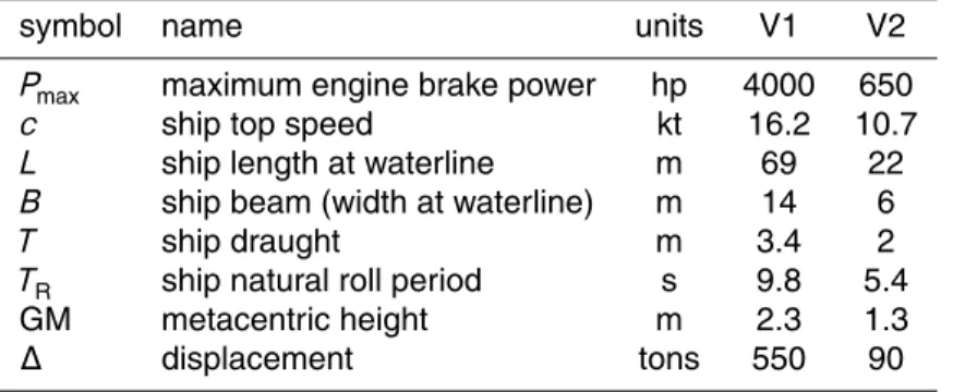
by factorizing the throttle dependence, as in the ship model by Perakis and Papadakis (1989). Furthermore, by comparing performances of vessel V1 (ferryboat) and V2 (fish-ing vessel) in Fig. 4, it can be seen that the former sustains a larger fraction of its top Froude number at any given significant wave height. This diﬀ_{erent dynamic behaviour}

is mainly related to the maximum engine brake power Pmax of the two vessels. This 15

is found by swapping just Pmax of the two vessels and keeping unchanged the other

parameters provided in Table 5 (not shown).

Figure 5 shows how the throttle needs to be adjusted to sustain a given speed in diﬀ_{erent sea states. An increase in speed requires an over-proportional increase in}

throttle. This leads, for each given sea state, to a so called “wave wall”

(MANDiesel-20

Turbo, 2011). Lloyd (1998) makes the assumption that the engine delivers constant power at a given throttle setting, regardless of the increased propeller load due to rough weather (note that propeller load is not considered in VISIR-I either). He then finds that the power required for sustaining a given speed steeply rises with wave height, similar to Fig. 5. The comparison between V1 and V2 also shows that the two vessels behave

25

very diﬀ_{erently in extreme seas, whereby vessel V1 (the ferryboat) is able to reach}

(20)

GMDD

8, 7911–7981, 2015

G. Mannarini et al.

Title Page

Tables Figures

◭ ◮

Back Close

Full Screen / Esc

Discussion

P

a

per

|

Discussion

P

a

per

|

Discussion

P

a

per

|

Discussion

P

a

per

|

Resistances are evaluated from the sustained speedv as:

Rc=ηk3v2 (25)

Raw=ηk2v (26)

and corresponding values are shown in Fig. 6.

While calm water resistance Rc does not explicitely depend on significant wave 5

heightHs,Rc depends on ship speed which, through Eqs. (22)–(24), depends on Hs.

Thus, assuming maximum throttle, a functional dependenceRc=Rc(Hs) can be

com-puted and is displayed in Fig. 6. Due to the fact thatk3is independent ofHs (Eq. 23),

calm water resistanceR_c is dominated by thev=_v(H_s_{) relationship seen in Fig. 4.}

Wave added resistanceRaw as a function ofHs initially grows quadratically and, for 10

higher waves, only linearly, Fig. 6. This is due to the combined eﬀ_{ect of the quadratic}

dependence on wave amplitude in k₂ (Eq. 24) and the nearly hyperbolic ship speed reduction for large Hs seen in Fig. 4. The same trend is observed in (Lloyd, 1998,

Fig. 3.13) and Nabergoj and Prpić_-Orš_ić_(2007).

In comparison to V2, vessel V1 exhibits larger resistances. However, for both vessel

15

classes, theRc andRaw curves form “scissors”, being wider for the larger vessel (V1),

Fig. 6.

2.3.3 Stability

The ship model described so far needs to be complemented by navigational constraints in order to reduce dangerous or unpleasant movements for the ship itself, the crew and

20

cargo.

Such situations cannot simply be ruled out by designing a vessel in accordance with the Intact Stability (IS) Code, IMO (2008). In fact, specific combinations of mete-orological and sea-state parameters may lead to dangerous situations even for ships complying with such mandatory regulations (Umeda, 1999; IMO, 2007). Furthermore,

25

(21)

GMDD

8, 7911–7981, 2015

G. Mannarini et al.

Title Page

Tables Figures

◭ ◮

Back Close

Full Screen / Esc

Discussion

P

a

per

|

Discussion

P

a

per

|

Discussion

P

a

per

|

Discussion

P

a

per

|

of the IS code obsolete. This led to the development of “second generation” stability criteria, being more physics and less statistics based than IS criteria.

VISIR-I checks for three modes of stability failure: parametric roll, pure loss of sta-bility, and surfriding/broaching-to. The theoretical hints below are mainly based on Be-lenky et al. (2011), while the implementation of the stability checks follows the

op-5

erational guidance by IMO more closely (IMO, 2007). In view of the limited angular resolution of the graph (Sect. 2.2.1), in VISIR-I stability in turning (Biran and Pulido, 2013) cannot be taken into consideration, and an unlimited vessel manoeuvrability (IMO, 2002) has to be assumed.

A realistic assessment of stability failure would require a detailed knowledge of ship

10

hull geometry. In the present version of VISIR-I, however, just principal particulars of the vessel (length, beam, draught) are employed. In addition, even vessel-internal mo-tions and mass displacements, such as the positioning of catch (Gudmundsson, 2009) and fuel sloshing (Richardson et al., 2005) may have an amplifying eﬀ_{ect on the loss}

of stability. Thus, the bare application of safety constraints described in the following

15

cannot guarantee navigation safety, and the ship-master should critically evaluate the resulting route computed by VISIR-I, also taking account the meteo-marine conditions actually met during the voyage and the specific vessel response.

In the following sections, we have used the deep water approximation in order to gain a rapid estimation of the threshold conditions. We can thus estimate the wavelength as:

20

λ[m]= g0

2πT

2

w≈1.56 (Tw[s])2 (27)

and the wave phase speed or celerity as:

cp[kt]= s

g0λ

2π ≈2.4

p

(22)

GMDD

8, 7911–7981, 2015

G. Mannarini et al.

Title Page

Tables Figures

◭ ◮

Back Close

Full Screen / Esc

Discussion

P

a

per

|

Discussion

P

a

per

|

Discussion

P

a

per

|

Discussion

P

a

per

|

Then, assuming a fully developed sea (Pierson–Moskowitz spectrum), the wave steep-ness can be estimated as:

Hs/λ=

2π g0

Hs

Tw2

= 8π

(24.17)2 ≈1/23 (29)

This result can be inferred from the plot of characteristic seas reported by Ström-Tejsen et al. (1973). For partially developed seas the wave steepness is larger and for dying

5

seas smaller than the value obtained in Eq. (29).

2.3.4 Parametric roll

When a ship is sailing in waves, the submerged part of the hull changes in time. For most hull shapes, this also involves a change in the waterplane area. This in turn influences the curve for the righting lever (GZ), which is fundamental to ship stability.

10

Indeed, if wavelengthλis comparable to ship lengthLand waves are met at a specific frequency, the change in GZ may trigger a resonance mechanism, leading to a dramatic amplification of roll motion (Belenky et al., 2011). A famous naval casualty ascribed to this mechanism of stability loss is reported in France et al. (2003).

The mathematical formulation of parametric roll is based on the solution of Mathieu’s

15

equations and the computation of Ince–Strutt’s diagram. It shows that parametric roll occurs when encounter wave periodTEsatisfies the condition

2TE=±nTR,n=1, 2, 3,. . . (30)

where TR is the ship’s natural roll period (Spyrou, 2005) and the ± sign in Eq. (30)

accounts for both following and head seas.

20

In VISIR-I the encounter periodTE is obtained by applying a Doppler’s shift to peak

wave periodTwand reads

TE=Tw·

1+ vcosα

3TwK(Tw,z) −1

(23)

GMDD

8, 7911–7981, 2015

G. Mannarini et al.

Title Page

Tables Figures

◭ ◮

Back Close

Full Screen / Esc

Discussion

P

a

per

|

Discussion

P

a

per

|

Discussion

P

a

per

|

Discussion

P

a

per

|

where Fenton’s factorK defined by Eq. (48) is used (vin kt). Instead, IMO’s formula for TE provided in (IMO, 2007, 1.6) corresponds to the deep water approximation, i.e. to

the caseK =_{1. Since in shallow waters and large wave periods}_{K <}_{1, IMO’s formula}

may lead to an overestimation ofTE.

Levadou and Gaillarde (2003) observe that a smaller GM also implies a larger natural

5

roll period TR and thus a parametric roll experienced in presence of longer waves.

Spyrou (2005) points out that, while any encounter angle α can in principle lead to parametric roll, vessels with low metacentric height GM (and, thus, largeTR) may be

more prone to experience parametric roll during following than head seas (due to larger |T_E_|).

10

Following (Levadou and Gaillarde, 2003) and the wave height criterion reported for L <100 m in Belenky et al. (2011), the parametric roll hazard condition is implemented in VISIR-I as:

0.8_≤λ/L_≤2 (32)

Hs/L≥1/20 (33)

15

together with Eq. (30) expressed in the form of the inequalities:

1.8_|TE| ≤TR≤2.1|TE| (34)

0.8|TE| ≤TR≤1.1|TE| (35)

where the coeﬃ_{cients in Eqs. (34)–(35) should be related to the roll damping}

charac-teristics of the vessel (Francescutto and Contento, 1999), but for the current version of

20

VISIR-I they are taken from Benedict et al. (2006).

Formula Eq. (31) shows thatTEperiod may be tuned by varying the speed and course

of the vessel. Thus, to prevent parametric rolling, a routing algorithm may suggest either a voluntary speed reduction or a route diversion. As shown in Sect. 2.2.3 and as will be seen in the case studies (Sect. 3), VISIR-I is able to exploit either option.

(24)

GMDD

8, 7911–7981, 2015

G. Mannarini et al.

Title Page

Tables Figures

◭ ◮

Back Close

Full Screen / Esc

Discussion

P

a

per

|

Discussion

P

a

per

|

Discussion

P

a

per

|

Discussion

P

a

per

|

2.3.5 Pure loss of stability

This mode of stability failure is triggered by a similar condition to the parametric roll. However, it does not involve any resonance mechanism and thus may be activated by a single wave. In fact, if the crest of a large wave is near the midship section of the ship, stability may be significantly decreased. If this condition lasts long enough (such

5

as during following waves and ship speed close to wave celerity), the ship may develop a large heel angle, or even capsize.

According to Belenky et al. (2011) a useful criterion for distinguishing ships prone to pure loss of stability involves a detailed knowledge of hull geometry. The IMO guid-ance (IMO, 2007) however proposes using just ship-wave kinematics. This is also the

10

criterion adopted in VISIR-I and can be stated as the following conditions to be simul-taneously verified:

λ/L_≥0.8 (36)

Hs/L≥1/25 (37)

|π−α| ≤π/4 (38)

15

1.3Tw≤v·cos(π−α)≤2.0Tw (39)

where ship speedv is given in kt.

Using also Eqs. (27)–(28) it can be seen that Eq. (39) implies (for exactly following seas) a sustained speedv between 43 and 67 % of wave celeritycp.

2.3.6 Surfriding/broaching-to

20

Surfriding is the condition where the wave profile does not vary relative to the ship. That is, the ship moves with a speed equal to wave celerity:v=_c_p_{. In this case, the}

ship is directionally unstable, with the possibility of an uncontrollable turn known as “broaching-to”.

(25)

GMDD

8, 7911–7981, 2015

G. Mannarini et al.

Title Page

Tables Figures

◭ ◮

Back Close

Full Screen / Esc

Discussion

P

a

per

|

Discussion

P

a

per

|

Discussion

P

a

per

|

Discussion

P

a

per

|

The simplest modelling of this mode of stability failure starts with the computation of the force of the wave-induced surge which is able to balance the diﬀ_{erence between}

total resistance and thrust provided by the ship. A critical point may then be reached, where surging is no longer possible and the ship is captured by the surfriding mode (Belenky et al., 2011). This phase transition is a heteroclinic bifurcation (Umeda, 1999).

5

In IMO (2007) a surfriding condition is proposed which just takes into account ship speed and length, independently of wave steepness. Based on numerical simulations, Belenky et al. (2011) overcomes this simplification, with the finding that the phase transition is less likely for less steep waves.

In VISIR-I, the following surfriding hazard criteria reported in Belenky et al. (2011)

10

are considered:

0.8_≤λ/L_≤2 (40)

Hs/λ≥1/40 (41)

|π−α| ≤π/4 (42)

F r·cos(π−α)≥F rcrit (43)

15

where the critical Froude number is given by

F r_crit=_0.2324(H_s_/λ)−1/3₋_0.0764(H_s_/λ)−1/2 ₍₄₄₎

Using Eq. (29) its typical value is found to be F rcrit=0.31. Condition Eq. (41) was

added to VISIR-I since F rcrit is reported in Belenky et al. (2011) just for the range

F r_∈[1/40, 1/8]. Condition Eq. (43) was complemented with anαdependence in

anal-20

ogy with Eq. (39) in order to account for following-quartering seas. This implies that surfriding is less likely to occur for quartering than following seas, sinceFris multiplied by a factor which may be as small as 1/√2.

Of note is that all VISIR-I safety constraints described above, Eqs. (32)–(43), are implemented in negative, i.e., as the set of conditions possibly leading to a stability

25

(26)

GMDD

8, 7911–7981, 2015

G. Mannarini et al.

Title Page

Tables Figures

◭ ◮

Back Close

Full Screen / Esc

Discussion

P

a

per

|

Discussion

P

a

per

|

Discussion

P

a

per

|

Discussion

P

a

per

|

2.4 Environmental fields

We distinguish the environmental fields between static (bathymetry and coastline) and dynamic fields (waves, winds, currents). In VISIR-I, bathymetry and coastline are em-ployed to ensure that navigation occurs in not too shallow waters and far from obstruc-tions. Of the dynamic fields, just wave forecast fields are used, as explained below.

5

2.4.1 Static fields

A 1/60◦(=_{1 Nautical Mile or 1 NM) bathymetry is used in VISIR-I. The dataset (NOAA}

Digital Bathymetric Data Base3) is used for a twofold purpose: (i) Along with the coast-line database, bathymetry is needed for computing a land–sea mask for safe naviga-tion. The first step is to select edges (jk) satisfying the condition that edge averaged

10

sea depthz=_(z_j+_z_k_{)/2 is larger than ship draught}_T_:

z > T (45)

In other words, for navigation just a strictly positive Under Keel Clearance UKC=_z₋_T

is admitted. (ii) Bathymetry is also needed for a more accurate estimation of wavelength λ, which is an important quantity for vessel stability checks of Sect. 2.3.3. Indeed deep

15

water approximation tends to overestimate λin shallow waters. Instead, VISIR-I em-ploys Fenton’s approximation (Fenton and McKee, 1990) which, upon the introduction of the deep water limitλ0for wavelength of the component of peak periodTw,

λ0=

g0

2πT

2

w (46)

3

http://www.ngdc.noaa.gov/mgg/bathymetry/iho.html

(27)

GMDD

8, 7911–7981, 2015

G. Mannarini et al.

Title Page

Tables Figures

◭ ◮

Back Close

Full Screen / Esc

Discussion

P

a

per

|

Discussion

P

a

per

|

Discussion

P

a

per

|

Discussion

P

a

per

|

can be rewritten as follows:

λ=_λ₀_·_K_(T_w_,z) ₍₄₇₎

K(Tw,z)= (

tanh

"

2πz λ0

3/4#)2/3

(48)

As seen from Eq. (48), in orderλto sense the eﬀ_{ect of shallow water,}_z_{should be small}

with respect to the scale set byλ0. 5

The coastline database is used in VISIR-I for a preliminary removal of the graph edge on the landmass (Sect. 2.2.1) and, jointly with the bathymetry, for the computation of a nautically safe land–sea mask (see below).

To this end, the NOAA Global Self-consistent, Hierarchical, High-resolution Geogra-phy Database (GSHHG4) is employed. Just two hierarchical levels are considered: the

10

coastline of the Mediterranean basin and its islands. The minimum distance between coastline data points is variable and is in some cases below 100 m.

A joint depth-coast land–sea mask is obtained by multiplying the mask defined by Eq. (45) with a mask of oﬀ_{shore grid points. Due to the quite di}ﬀ_{erent spatial resolution}

of the coastline and the environmental fields, a regridding procedure is employed for

15

reconstructing the coastal fields:

1. Fields are extrapolated inshore by replacing missing values of sea fields with the average of the first neighbouring grid points, Fig. 7. This “sea-over-land” proce-dure is distinguished by the extrapolation used in De Dominicis et al. (2013) by: the number of neighbours used (8 and not just 4) and the absence of the condition

20

that at least two neighbouring grid points have assigned field values. Sea-over-land can be iterated in order to define field values on further neighbouring Sea-over-land grid points.

4

(28)

GMDD

8, 7911–7981, 2015

G. Mannarini et al.

Title Page

Tables Figures

◭ ◮

Back Close

Full Screen / Esc

Discussion

P

a

per

|

Discussion

P

a

per

|

Discussion

P

a

per

|

Discussion

P

a

per

|

2. The fields are bi-linearly interpolated to the target grid. In VISIR-I this is the bathymetry grid. Thus, spatial resolution of wave fields is enhanced from the orig-inal 1/16 to 1/60◦.

2.4.2 Dynamic fields

The dynamic environmental fields are used in VISIR-I for the computation of sustained

5

ship speeds and safety constraints. In the present version, just the eﬀ_{ect of waves}

is considered, which is deemed to be the most relevant for medium and small-size vessels. The eﬀ_{ect of wind and sea currents is planned for future development:}

1. Wind drag may be significant for vessels with a large freeboard and/or superstruc-ture area (Hackett et al., 2006);

10

2. Sea current drift is relevant especially in proximity to strong ocean currents (Takashima et al., 2009) and for not too fast vessels with large draughts;

3. Wave eﬀ_{ects include both drift and involuntary speed reduction. The drift is due to}

nonlinear mass transport in waves (Stokes’drift, Newman, 1977). It is small when the reduced wavenumber L/λ is smaller than unity and increases significantly

15

when L/λ_≈1 (Hackett et al., 2006). Involuntary speed reduction in waves was instead detailed in Sect. 2.3.

Thus, the eﬀ_{ect of wind drag may be neglected for not too large vessels, and the e}ﬀ_ect

of current and wave drift for vessels able to sustain significantly larger speeds than the current magnitude. In addition, since coastal wave fields may be aﬀ_{ected by the} extrap-20

olation/interpolation procedure, and due to the current resolution of the bathymetry grid (1 NM) (Sect. 2.4.1), also very small vessels, sailing coastwise on short routes, should be removed from the scope of this system. Thus, we roughly estimate the range of admissible vessel lengthsLto be up to a few tens of meters.

The current version of VISIR-I employs wave forecast fields from an operational

im-25