www.atmos-chem-phys.net/8/3081/2008/ © Author(s) 2008. This work is distributed under the Creative Commons Attribution 3.0 License.
Chemistry
and Physics
Impact of nonlinearity on changing the a priori of trace gas profile
estimates from the Tropospheric Emission Spectrometer (TES)
S. S. Kulawik1, K. W. Bowman1, M. Luo1, C. D. Rodgers2, and L. Jourdain1
1Jet Propulsion Laboratory, California Institute of Technology, Pasadena, CA, USA 2University Oxford, Clarendon Lab, Oxford OX1 3PU, UK
Received: 18 October 2007 – Published in Atmos. Chem. Phys. Discuss.: 25 January 2008 Revised: 16 May 2008 – Accepted: 26 May 2008 – Published: 20 June 2008
Abstract. Non-linear maximum a posteriori (MAP) esti-mates of atmospheric profiles from the Tropospheric Emis-sion Spectrometer (TES) contains a priori information that may vary geographically, which is a confounding factor in the analysis and physical interpretation of an ensemble of profiles. One mitigation strategy is to transform profile es-timates to a common prior using a linear operation thereby facilitating the interpretation of profile variability. However, this operation is dependent on the assumption of not worse than moderate linearity near the solution of the non-linear estimate. The robustness of this assumption is tested by comparing atmospheric retrievals from the Tropospheric Emission Spectrometer processed with a uniform prior with those processed with a variable prior and converted to a uni-form prior following the non-linear retrieval. Linearly con-verting the prior following a non-linear retrieval is shown to have a minor effect on the results as compared to a non-linear retrieval using a uniform prior when compared to the expected total error, with less than 10% of the change in the prior ending up as unbiased fluctuations in the profile esti-mate results.
1 Introduction
Optimal estimation is a powerful technique for performing atmospheric retrievals because of its capability to character-ize errors and sensitivity (Rodgers, 2000; Bowman et al., 2006). This characterization allows data to be assimilated into chemistry and transport models (Jones et al., 2003) com-pared to other datasets (Rodgers and Connor, 2003; Worden
Correspondence to:S. Kulawik ([email protected])
et al., 2007), and prior vectors to be changed (Rodgers and Connor, 2003). However, these approaches are based on the assumption that the retrieved atmospheric state is spectrally linear with respect to the “actual” atmospheric state, i.e. that a linear expansion of the forward model is accurate between the retrieved and true atmospheric states to significantly bet-ter than predicted errors. We test the impact of this linearity assumption on post facto linear operations on TES retrievals such as “swapping” the a priori profile.
Using the most accurate prior will lead to the most ac-curate results; however conversion to a uniform prior can be useful for scientific analysis, such as highlighting sea-sonal cycles, comparing observations from two different re-gions that may have different priors, or comparing results from different satellites. Recent papers which have used TES data linearly converted to a uniform prior include Zhang et al. (2006) who examined the global distribution of TES ozone and carbon monoxide correlations in the middle tro-posphere, Logan et al. (2008) who studied the effects of the 2006 El Nino on carbon monoxide, ozone, and water, and Luo et al. (2007) who compared TES and the Measurements of Pollution in the Troposphere (MOPITT) instrument car-bon monoxide results and explores the influence of the a pri-ori. MOPITT processing currently uses a uniform prior to reduce artefacts arising from the prior and maximize the im-pact of the satellite data (Deeter et al., 2003).
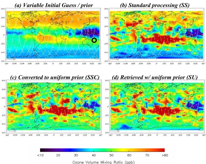
(a) Variable Initial Guess / prior
(b) Standard processing (SS)
(c) Converted to uniform prior (SSC)
(d) Retrieved w/ uniform prior (SU)
Fig. 1. TES retrieved ozone at 681 hPa. Panel(a)shows the standard globally variable TES a priori and initial states, with observation location shown with white +’s. Panel(b)shows the TES standard retrieval (SS). Panel(c)shows the TES standard retrieval converted to a uniform prior (SSC). Panel(d)shows TES retrieved with a uniform prior (SU). Panels (c) and (d) should agree in the linear regime. The circle in panel (a) shows the value of the uniform prior at this pressure which is 48 ppb. The color scale, which is the same for all plots, is shown below all 4 plots.
ozone (H. Worden et al., 2007; Nassar et al., 2008; Osterman et al., 2008; Richards et al., 2008), carbon monoxide (Rins-land, 2006; Luo et al., 2007a, b), and methane, as well as surface temperature, emissivity, and cloud information (El-dering et al. 2008). For details on the TES instrument, see Beer et al., 2006, and for information on the retrieval pro-cess see Bowman et al. (2006) and Kulawik et al. (2006a). TES products and documentation are publicly available from the Langley Atmospheric Science Data Center (ASDC), http: //eosweb.larc.nasa.gov/PRODOCS/tes/table tes.html
The TES retrieval strategy is briefly listed to give the reader the context of the TES retrievals of ozone, carbon monoxide, and methane for v003 data. (1) The first retrieval step is a cloud detection step which compares the observed and calculated brightness temperatures in the 11 um region and sets the initial cloud optical depth, and an initial cloud retrieval step is done if the estimated cloud optical depth is large. (2) Atmospheric temperature, water, ozone, surface
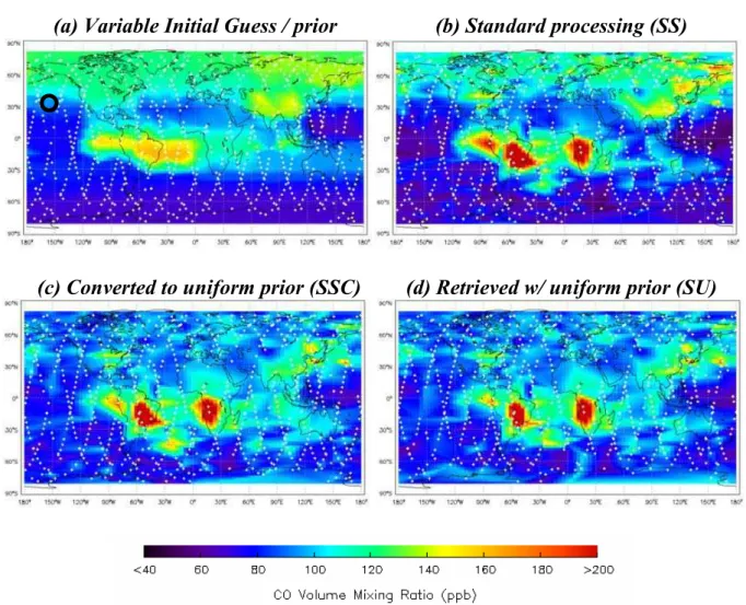
(a) Variable Initial Guess / prior
(b) Standard processing (SS)
(c) Converted to uniform prior (SSC)
(d) Retrieved w/ uniform prior (SU)
Fig. 2. TES retrieved carbon monoxide at 681 hPa. Panel(a)shows the variable TES a priori. Panel(b)shows the TES standard retrieval (SS). Panel(c)shows the TES standard retrieval converted to a uniform prior (SSC). Panel(d)shows TES retrieved with a uniform prior (SU). Panels (c) and (d) should agree in the linear regime. The circle in panel (a) shows the approximate value of the uniform prior at this pressure (97 ppb).
-120
-60
0
60
120
-120
-60
0
60
120
-60
-30
0
30
60
-60
-30
0
30
60
O3 VMR Fraction at 681 hPa
-0.250
-0.125
0.000
0.125
0.250
-120
-60
0
60
120
-120
-60
0
60
120
-60
-30
0
30
60
-60
-30
0
30
60
CO VMR Fraction at 681 hPa
Difference at 681.3 hPa
-0.4
-0.2
0.0
0.2
0.4
VMR fractional difference
0
10
20
30
40
50
# cases (%)
Bias: 0.01
3
σ
: 0.15
78% w/in 5% err
n = 648
Difference at 177.8 hPa
-0.4
-0.2
0.0
0.2
0.4
VMR fractional difference
0
10
20
30
40
50
# cases (%)
Bias: -0.00
3
σ
: 0.26
69% w/in 5% err
n = 651
Difference at 38.3 hPa
-0.4
-0.2
0.0
0.2
0.4
VMR fractional difference
0
10
20
30
40
50
# cases (%)
Bias: 0.01
3
σ
: 0.12
78% w/in 5% err
n = 651
RMS profile Difference
0.0
0.1
0.2
0.3
0.4
0.5
VMR fractional diff
0
10
20
30
40
50
# cases (%)
3
σ
: 0.18
64% w/in 5% err
n = 651
(c)
(d)
(a)
(b)
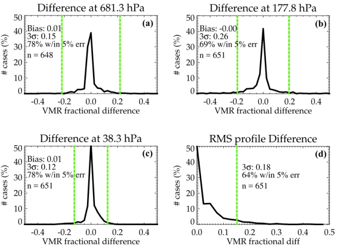
Fig. 4. Statistical comparison between non-linear retrievals using a uniform prior (SU) vs. conversion to a uniform prior using Eq. (??) (SSC). The black line shows the histogram of the Fractional difference of (SSC – SU) for 3 different pressure levels. The green dashed line is the mean TES reported total error. The lower right plot is the standard deviation of the VMR fractional difference averaged over the entire profile.
A retrieved profile can be expressed as a first order expan-sion in(x−xa)(Rodgers, 2000; Bowman et al., 2002):
ˆ
x=xa+A(x−xa)+ε (1)
wherexa, xˆ, and x are the prior, retrieved, and true
pro-file state in log(volume mixing ratio (VMR)),Ais the av-eraging kernel matrix (Backus and Gilbert, 1970; Rodgers, 2000) which describes the sensitivity of the retrieval to the true state, and ε represents the error resulting from spec-tral noise, spectroscopic errors, cross-state error, and inac-curacies of non-retrieved species, as discussed in Worden et al. (2004).
Adjustment to a new prior can be done using the following equation (Rodgers and Connor, 2003):
ˆ
x′=xˆ+(A−I)(xa−xa′) (2)
wherexaandxa′ are the original and new priors, respectively, ˆ
xis the original retrieved value, andxˆ′is the retrieved value with the new prior. Equation (2) shows that when averaging kernel matrix,A, is unity then changes to the prior have no effect on the retrieved value. Conversely when the averaging
kernel matrix is zero, Eq. (1) shows that the retrieved state is equal to the prior. The averaging kernel is almost always somewhere in between these two extremes for atmospheric retrievals. In the case of TES, the retrieval vectorxˆ includes
not only the trace gas of interest, but also surface and cloud properties, and for the ozone retrieval, also water and temper-ature. Whenx′
ais modified for only the trace gas of interest,
Eq. (2) shows that the propagation toxˆ′ for the trace gas of
interest is the same whether the full retrieval vector is con-sidered or whether the matrices and vectors in Eq. (2) refers to just the trace gas of interest.
Equation (1) assumes not worse than moderate non-linearity between the retrieved state and the true state while Eq. (2) assumes not worse than moderate non-linearity be-tween the two retrieved states (Rodgers 2000). As a conse-quence, the averaging kernel derived from a non-linear op-timal retrieval with a priori,xa, should be sufficiently close
to an averaging kernel derived from a non-linear optimal re-trieval with a priori,x′
a. This linearity assumption is tested
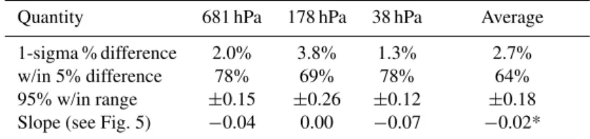
af-Table 1.Summary of the differences between the linear vs. non-linear application of a uniform prior for ozone.
(a) all good quality cases
Quantity 681 hPa 178 hPa 38 hPa Average
1-sigma % difference 2.0% 3.8% 1.3% 2.7%
w/in 5% difference 78% 69% 78% 64%
95% w/in range ±0.15 ±0.26 ±0.12 ±0.18
Slope (see Fig. 5) −0.04 0.00 −0.07 −0.02*
(b) screened by convergence which is indicated by the initial guess results
Quantity 681 hPa 178 hPa 38 hPa Average
1-sigma % difference 1.1% 1.6% 1.0% 0.7%
w/in 5% difference 95% 88% 94% 90%
95% w/in range ±0.06 ±0.12 ±0.05 ±0.06
slope 0.01 0.01 −0.02 −0.01*
∗The slope is calculated for the mean difference of the profiles. The other average quantities are calculated for the rms difference.
Table 2. Summary of the differences between the linear vs. non-linear application of a uniform prior for carbon monoxide.
Quantity 681 hPa 383 hPa Average
1-sigma 0.8% 2.0% 1.1%
w/in 5% difference 89% 87% 88%
95% w/in range ±0.09 ±0.10 ±0.22
Slope 0.02 0.07 0.02*
∗The slope is calculated for the mean difference of the profiles. The
other average quantities are calculated for the rms difference.
fect the solution as long as that solution represents the global minimum. On the other hand, if a local minimum is reached, then neither Eq. (1) nor Eq. (2) may be valid and the esti-mated profile will depend on the choice of the initial guess. The dependency of the retrieval on the initial guess is tested as well by also comparing standard retrievals to those that are retrieved using a globally constant initial guess.
Additionally, the reader should be aware that the choice of prior will affect the predicted error in the retrieval through the smoothing error component, which depends on the a priori covariance matrix. The a priori covariance matrix is the ex-pected covariance between the prior and the true state; if the global mean is chosen as the prior, the variance between the prior and the true state will increase as compared to choosing a more accurate prior that depends on latitude and longitude. It is apparent in Figs. 1 and 2 that the errors in the estimated state are much larger for the globally uniform prior than for the original prior, especially in the polar region where sen-sitivity is less and the prior has changed a great deal. The increased errors will be the same whether the profile was re-trieved non-linearly or estimated using Eq. (2).
Table 3. Summary of the differences between the linear vs. non-linear application of a uniform prior for methane.
Quantity 287 hPa Average
1-sigma 0.3% 0.3%
w/in 5% difference 100% 100% 95% w/in range ±0.01 ±0.02
slope −0.01 −0.01*
∗The slope is calculated for the mean difference of the profiles. The
other average quantities are calculated for the rms difference.
2 Method
One day’s worth of data from the TES instrument, consisting of 1152 globally distributed profiles taken 20–21 September 2004, was processed in three different ways with the dataset designation shown in parentheses:
1. standard processing with variable initial guess and prior (SS)
2. processing with variable initial guess and uniform prior (SU)
3. processing with uniform initial guess and variable prior (US)
4. standard processing converted linearly to a uniform prior using Eq. (2) (SSC)
Difference vs. prior, stddev
0
20
40
60
80
100 120
O3 (%) prior: SS - US
0
20
40
60
80
O3 (%) result: SS - US
slope: 0.08
Difference vs. prior, mean
-50
0
50
O3 (%) prior: SS - US
-20
-10
0
10
20
O3 (%) result: SS - US
slope: -0.02
(a)
(b)
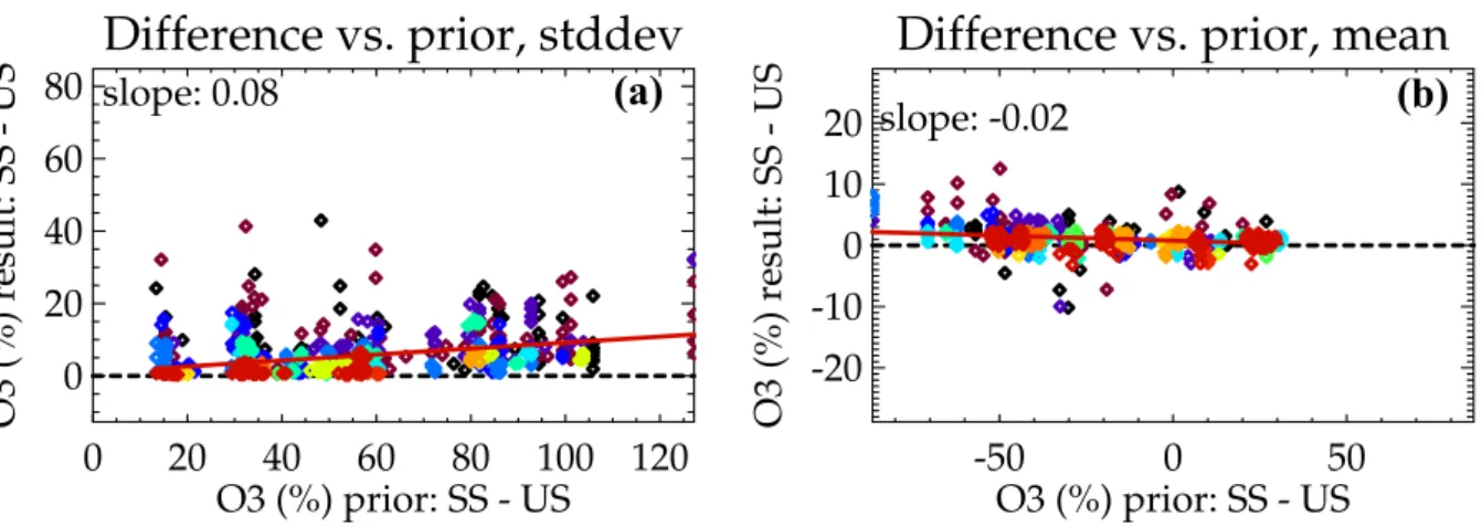
Fig. 5.Change in (SSC-SU) as a function of the change in the prior. The colors represent density of points using the same color progression as used in Figs. 1 and 2, where red indicates the highest density of points. The calculated slope is shown as a red line. These results indicate that less than 10% of the prior’s change will end up as unbiased fluctuations in the answer.
Difference at 681.3 hPa
-0.4
-0.2
0.0
0.2
0.4
VMR fractional difference
0
10
20
30
40
50
# cases (%)
Bias: 0.05
3
σ
: 0.81
67% w/in 5% err
n = 648
Difference at 177.8 hPa
-0.4
-0.2
0.0
0.2
0.4
VMR fractional difference
0
10
20
30
40
50
# cases (%)
Bias: -0.12
3
σ
: 0.87
62% w/in 5% err
n = 651
(a)
(b)
Fig. 6.Statistical comparison between non-linear retrievals using a globally constant initial guess vs. variable initial guess. The black line shows the histogram of the VMR fractional difference for SS-US for 2 different pressure levels (681 and 178 hPa).
and the prior are the same and vary by latitude and longitude as described below. For dataset SSC, the standard process-ing (SS) result is converted to a global uniform prior usprocess-ing Eq. (2). Datasets SSC and SU should be equivalent; assum-ing Eq. (2) is valid. Similarly, datasets SS and US should be equivalent since, as seen in Eq. (1), the initial guess should not impact the final answer, assuming convergence to the global minimum is achieved. For the global uniform prior or initial guess, the global average was created by taking a linear average over all priors or initial guesses for the run. The initial guess and prior for atmospheric temperature, sur-face temperature, and water are taken from the Global Model Assimilation Office (GMAO) (Rienecker et al., 2006). For ozone, carbon monoxide, and methane, the prior/initial guess are taken from a climatological MOZART-3 run (Brasseur et al., 1998; Park et al., 2004) which has averages binned by latitude and longitude bands (typically 10–30 degree latitude bands and 60 degree longitude bands).
To compare datasets quantitatively, histograms were made of the fractional differences defined as:
fractional difference=xˆ1−xˆ2 (3) Sincexˆrepresents Log(VMR), a value of 0.10 for the
frac-tional difference indicates a 10% difference.
We also plot differences between (SSC-SU) versus the amount of change in the prior, which shows whether there is a breakdown in the accuracy of the results if changes to the prior are too large, and shows whether changes in the prior introduce biases in the result. Linear regression is used to calculate the slope of differences between (SSC-SU) versus the change in the prior.
Difference at 681.3 hPa
-0.4
-0.2
0.0
0.2
0.4
VMR fractional difference
0
10
20
30
40
50
# cases (%)
Bias: 0.01
3
σ
: 0.06
95% w/in 5% err
n = 371
Difference vs. prior, stddev
0
20
40
60
80
100 120
O3 (%) prior: SS - US
0
20
40
60
80
O3 (%) result: SS - US
slope: 0.04
(a) (b)
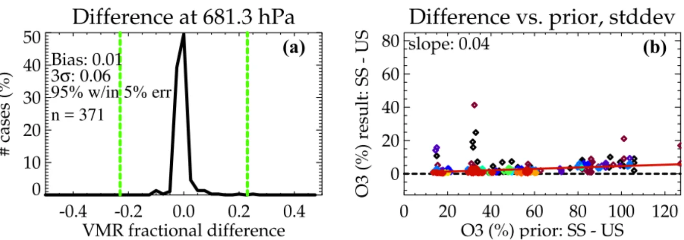
Fig. 7.The effects of removing outliers on the prior comparison. Cases which are outliers from swapping the initial guess are removed from the prior comparison. The remaining cases show better characteristics compared to Figs. 4 and 5.
3 Results
A TES global survey consisting of 1152 globally distributed nadir observations from 20–21 September 2004 was run for three different configurations for the prior and initial guess, as described in the methods section. Following the non-linear retrievals, the standard retrieval dataset (SS) was converted to the fixed prior dataset (SSC) using Eq. (2).
Figures 1 and 2 show the initial and retrieved values at 681 hPa for ozone and carbon monoxide, respectively, for datasets SS, SU, and SSC. The TES nadir observation lo-cations are shown with white +’s and interpolation is done between the TES observation locations. The TES standard prior for both figures (panel a) is taken from a climatological run of the MOZART-3 model binned by 60 degrees longi-tude, and 10 degrees latitude. For the ozone prior, shown in Fig. 1, panel (a), enhancements are seen in the Northern lat-itudes (>60 N) and an enhanced band from South America through southern Africa to Australia (the biomass burning region (discussed in Bowman et al., 2008)), and a minimum is seen north of Australia. The standard retrieval shown in Fig. 1b represents these same patterns with a marked en-hancement in the biomass burning region. The constant prior cases (panels c and d) agree remarkably well with each other indicating that the linearly converting the prior is valid throughout most of the data. The features in panels c and d can be confidently attributed to the TES data without precon-ceptions introduced by the prior; however large differences between panels (b) and (c) or (d) indicate a dependence on the prior rather than the data. The absence or presence of par-ticular points passing quality flags can cause minor changes in the three different results. Most of ozone enhancements between 60 S–60 N remain between the standard processing and the converted prior (Fig. 1b and c) indicating that TES re-trievals are sensitive at this pressure level over those regions. Poleward of 60 N, patterns seen in the original prior and the standard retrieval are absent, indicating that TES retrievals are insensitive in those regions.
Figure 2 show the same plots as in Fig. 1, for carbon monoxide. The carbon monoxide prior (Fig. 2a) indicates enhancement over South America and southern Africa (in the biomass burning region), north of 40 N, and over India and southeast Asia. The standard retrieval Fig. 2b displays marked enhancement over the prior in eastern South Amer-ica and western sub-Sahara AfrAmer-ica, and in eastern Asia. The uniform prior results, panels (c) and (d), show good agree-ment with each other. The East Asia enhanceagree-ment is present but muted and the pattern and values in the biomass burn-ing region are very similar between panels (b), (c), and (d), however the CO enhancement poleward of 40 N is markedly reduced in (c) and (d) indicating that TES retrievals have less sensitivity in those regions.
Figure 3 shows global maps of the VMR fractional differ-ence (using Eq. 3) for O3 and CO at 681 hPa for the SSC and SU datasets. The plots show that outliers occur predom-inately in the tropics, and to a lesser extent, Antarctica. The pattern may suggest two cloud layers, which occur frequently in the tropics (Zipser, 1969), could contribute to the retrieval variation since TES assumes one cloud layer (Kulawik et al., 2006b), however determining correlations between outliers and atmospheric conditions was not explored further in this paper.
3.1 Statistical analysis
To quantify differences, statistical analysis was done on the 681 observations which have good quality flags for all three runs (SS (and by extension SSC), SU, and US). The master quality flag is set to screen out about 80% of the bad cases, but will also screen out perhaps 20% of good cases as well (Osterman et al., 2006).
within 5% of each other, (2) the fractional difference that encompasses 95% of the observations, and (3) the standard deviation of the fractional difference.
3.1.1 Results for ozone
In Fig. 4, a histogram of the VMR fractional difference, us-ing Eq. (3), is shown comparus-ing dataset SSC (the standard retrieval converted to a uniform prior using Eq. (2) to SU (the non-linear retrieval using a uniform prior) at 681, 178, 38 hPa, and over the entire profile. Figure 4 shows that for ozone, 70–80% of the SSC and SU results are within 5% dif-ference. It is not surprising that histogram for the 177.8 hPa pressure level has the widest spread among the 3 pressure levels chosen because ozone at that pressure level has an order of magnitude variability due to the variations in the tropopause height; a globally constant value for ozone be-tween 100–300 hPa is very challenging to the retrieval. Note that the errors introduced by changing the prior are small when compared to the TES reported total error (green dashed line in Fig. 4). In comparison, the VMR fractional difference of the prior had a 1-sigma value of 0.41, 1.08 (i.e. 108%), and 0.16 at 681, 178, and 38 hPa, respectively, indicating signifi-cantly more spread in the prior than in the resulting retrieval. The 1-sigma values for the results are shown in Table 1.
The histograms in Fig. 4 all show sharp peaks centered near zero but also show more outliers than would be expected from a Gaussian distribution. To determine if the outlying points are a result of a breakdown in the linear transform in Eq. (2) that occurs when the a priori change is too large, the difference (SSC-SU) is plotted versus the change in the prior, averaged over the profile, in Fig. 5. Figure 5 shows no obvious difference between small and large prior changes. In Fig. 5, panel (a) shows the rms of (SSC-SU), and panel (b) shows the mean difference, both averaged over the entire profile. For the rms difference, the slope tells whether, on av-erage, larger differences in the prior lead to larger differences in the results. This slope was 0.10. For the mean difference, the slope indicates if changes in the prior are correlated with the error in Eq. (2) predictions. If a positive slope is found, it would indicate that sensitivity is significantly increased at the new convergence location compared to the old location when the change in the prior is positive. The slope of the mean difference was found to be−0.02. Together these
re-sults mean that the error in the answer will be less than 10% of the prior’s change, and will be unbiased with respect to the prior’s direction of change. The lack of bias suggests that the differences are not a function of the choice of the uniform prior; further testing with a globally uniform initial guess in the next section strengthens this conclusion.
To check whether the outliers in Fig. 4 are a result of con-verging to a different local minimum, a run was done with a globally uniform initial guess (dataset US). The initial guess is the starting location for the retrieval, which iterates un-til convergence is reached. Since the initial guess is not
in-cluded in the cost function, which determines the final solu-tion, it should not affect the retrieval assuming the retrieval gets to the global minimum. However, an initial guess far from true can lead the retrieval to a non-global minimum, and systematic errors in the forward model or observed radiance can roughen the error landscape and introduce local minima. A more complete description of TES retrievals is discussed in Bowman et al. (2006). Theoretically, the initial guess does not influence the results (as seen also in Eq. 1) and dataset US should converge to the same answer as the standard retrieval (dataset SS). Differences in these datasets indicate conver-gence to different local minima, but we do not know whether either has reached a global minimum. The histograms from this run for ozone are shown in Fig. 6. In general, histograms of SS vs. US show a sharper peak and more outliers than the histograms from Fig. 4. For O3at 681 hPa, for example, 17% of observations change greater than the TES reported error compared to 2% for results shown in Fig. 4.
Figure 7 has all “initial guess outliers” removed, and com-pares remaining observations for datasets SSC and SU. “Ini-tial guess outliers” are set to be those where the average rms difference over the profile between SS and US were more than 5%, and represent observations that show a tendency to converge to different minima. Results are shown in Fig. 7 for 681 hPa, and correlations shown for the profile standard deviation. In this case, there are significantly fewer outliers (compared to Figs. 4 and 5). The right plot in Fig. 7 shows that the spread in the prior is still about the same, but that the spread in the result is markedly less. This means that the out-liers in Figs. 4 and 5 likely result from retrievals converging to different local minima. Table 1 summarizes the results for Figs. 4, 5, and 7 for ozone.
As discussed following Eq. (2), when a retrieval is not sen-sitive, it will converge to the prior and exchanging the prior will move the retrieval to the new prior, as seen for retrievals poleward of 60 N in Fig. 1. The effects of changing the prior on the most sensitive points is of interest, so statistics were calculated for only those points with a corresponding aver-aging kernel diagonal value of 0.04 or greater (retaining only the most sensitive half of the data). For 681 hPa, the num-ber of samples dropped from 648 to 290; the bias increased from 0.01 to 0.02, the 1-sigma value increased from 2.0% to 2.7%, the 3-sigma value increased from 15% to 17%, and the fraction within 5% error dropped from 78% to 65%. For 177.8 hPa and 38.3 hPa, the changes are smaller, for exam-ple for 38.3 hPa the fraction within 5% error dropped from 78% to 72%. However the result that the error is unbiased and smaller than the reported total error still holds true for the most sensitive points.
3.1.2 Results for carbon monoxide
Difference at 681.3 hPa
-0.2
-0.1
0.0
0.1
0.2
VMR fractional difference
0
10
20
30
40
50
# cases (%)
Bias: 0.01
3
σ
: 0.09
89% w/in 5% err
n = 587
Difference at 383.1 hPa
-0.2
-0.1
0.0
0.1
0.2
VMR fractional difference
0
10
20
30
40
50
# cases (%)
Bias: 0.01
3
σ
: 0.10
87% w/in 5% err
n = 590
RMS profile Difference
0.00
0.05
0.10
0.15
0.20
VMR fractional diff
0
10
20
30
40
50
# cases (%)
3
σ
: 0.22
88% w/in 5% err
n = 590
Difference vs. prior, mean
-40
-20
0
20
40
CO (%) prior: SS - US
-40
-20
0
20
40
CO (%) result: SS - US
slope: 0.02
(c)
(d)
(a)
(b)
Fig. 8. Statistical comparison for carbon monoxide between non-linear retrievals using a uniform prior vs. conversion to a uniform prior using Eq. (2). The black line shows the histogram of the VMR fractional difference of SSC and SU using Eq. (3) for 2 different pressure levels for carbon monoxide. The lower right panel shows the mean change in the result vs. the mean change in the prior.
or cloud parameters resulting from the uniform ozone prior will propagate into differences in the carbon monoxide step. Swapping only the carbon monoxide, rather than all the species together, may improve on the results shown in this study. Figure 8 shows the histogram of the fractional VMR change for CO at 383 and 681 hPa (note Figs. 8 and 9 do not have initial guess outliers removed). Additionally results are shown for averages over the entire profile. Carbon monox-ide shows fewer outliers beyond 10% than found with ozone. Results for CO are summarized in Table 2. In comparison, the VMR fractional difference of the prior had a 1-sigma value of 0.30 and 0.17 at 681 and 381 hPa, respectively, in-dicating significantly more spread in the prior change than in the resulting retrieval.
3.1.3 Results for methane
Methane is also retrieved following the tempera-ture/water/ozone steps, and changes to the temperature, surface temperature, or cloud parameters resulting from the uniform ozone prior will propagate into differences in the methane step. The results seen in this study are likely to be
worse than the results from swapping only the methane. Fig-ure 9 shows results at 287 hPa and for the whole profile, and shows that changing to a uniform prior results in less than a 1% difference in methane for 95% of the cases. Results for methane are summarized in Table 3. In comparison, the VMR fractional difference of the prior had a 1-sigma value of 0.06 at 287 hPa indicating significantly more spread in the prior change than in the resulting retrieval.
Difference at 287.3 hPa
-0.10
-0.05
0.00
0.05
0.10
VMR fractional difference
0
10
20
30
40
50
# cases (%)
Bias: -0.00
3σ
: 0.01
100% w/in 5% err
n = 615
RMS profile Difference
0.00
0.02
0.04
0.06
0.08
0.10
VMR fractional diff
0
10
20
30
40
50
# cases (%)
3
σ
: 0.02
100% w/in 5% err
n = 615
Difference vs. prior at 287 hPa
-50
0
50
CH4 (ppb) prior: SS - SU
-50
0
50
CH4 (ppb) result: SS - SU
slope: -0.01
Difference vs. prior, stddev
0
10
20
30
40
50
60
CH4 (%) prior: SS - US
0
10
20
30
40
CH4 (%) result: SS - US
slope: 0.03
(c)
(d)
(a)
(b)
Fig. 9.Statistical comparison for methane between non-linear retrievals using a uniform prior vs. conversion to a uniform prior using Eq. (2). The black line shows the histogram of the Fractional difference using Eq. (3) of SSC-SU for 287 hPa. The red line shows the histogram of the differences in the priors, which show significantly more spread. The upper right panel shows the histogram of the average error for all pressures. The lower right panel shows the difference in the retrieval result vs. the difference in the prior for 287 hPa, and the lower right is the same for the mean difference over the whole profile.
For ozone, the mean degrees of freedom for signal (DOF) is 3.80. The mean DOF changes 0.01 between the two runs. The rms difference of the DOF is 0.04, which is about 1%. The mean value of the averaging kernel diagonal between the surface and 10 hPa is 0.069. The mean difference between the two runs is 8×10⁻⁵, and the rms fractional difference of
the averaging kernel diagonals are 15%.
For retrievals in Log(VMR), sensitivity is positively cor-related to the VMR (Deeter et al., 2007). Retrievals with a 10% increase in the retrieved ozone column density also have about a 0.15 increase in the degrees of freedom, a 4% increase. Since the uniform prior is set to the global mean, this does not cause a biased change between the two runs for this test.
For carbon monoxide, the mean DOF is 1.09, with a mean difference of 0.004 between the two runs. The rms difference is 0.02, or 2%. The mean value of the averaging kernel di-agonal between the surface and 10 hPa is 0.039. The mean difference between the two runs is 0.0006, and the rms frac-tional difference of the averaging kernel diagonals are 22%.
For methane, the mean DOF is 1.27, with a mean differ-ence of 8×10⁻⁶ between the two runs. The rms difference
is 0.04, or 3%. The mean value of the averaging kernel di-agonal between the surface and 10 hPa is 0.024. The mean difference between the two runs is 0.00003, and the rms frac-tional difference of the averaging kernel diagonals are 12%.
For all three species, the total DOF varies by less than 3% when the prior is changed, and the individual averaging kernel diagonal values vary by about 20%. This indicates that the error bars and sensitivities may have about a 20% unbiased change for any particular level when the prior is changed, however the total DOF remains fairly impervious to changes in the prior.
4 Conclusions
prior, when compared to the expected total error. Histograms of differences between these two methods show a sharp peak centered near zero with some outliers, especially for ozone. Further analysis of the characteristics of the outliers, and comparisons to retrievals with a uniform initial guess indi-cates that the many of the outliers result from convergence to a local minimum rather than breakdown of the linear con-version in Eq. (2). For ozone, the 1-sigma difference is less than 4% for each of three pressure levels studied, and the mean change for all levels is 2.7%. For methane, the 1-sigma change is 0.3% at 287 hPa and 0.3% for the profile aver-age, and for carbon monoxide the 1-sigma change is about 2%. The degrees of freedom comparison between shows a 1-sigma difference of less than 3% for all the species, and shows changes of the averaging kernel diagonal are on the order of 20% for individual levels.
Acknowledgements. Thanks to members of the TES science team
and the TES software team. This work was performed at the Jet Propulsion Laboratory, California Institute of Technology, under a contract with the National Aeronautics and Space Administration.
Edited by: U. P¨oschl
References
Backus, G. and Gilbert, F.: Uniqueness in Inversion of Inaccurate Gross Earth Data, Philos. Tr. R. Soc. S-A, 266(1173), 123–192, 1970.
Beer, R.: TES on the Aura mission: Scientific objectives, measure-ments, and analysis overview, IEEE T Geosci. Remote, 44(5), 1102–1105, 2006.
Bowman, K. W., Worden, J., Steck, T., Worden, H. M., Clough, S. and Rodgers, C.: Capturing time and vertical variability of tropo-spheric ozone: A study using TES nadir retrievals, J. Geophys. Res.-Atmos., 107(D23), 4723, doi:10.1029/2002JD002150, 2002.
Bowman, K. W., Rodgers, C. D., Kulawik, S. S., Worden, J., Sarkissian, E., Osterman, G., Steck, T., Lou, M., Eldering, A., Shephard, M., Worden, H., Lampel, M., Clough, S., Brown, P., Rinsland, C., Gunson, M., and Beer, R.: Tropospheric emis-sion spectrometer: Retrieval method and error analysis, IEEE T Geosci. Remote, 44(5), 1297–1307, 2006.
Bowman, K. W., Jones, D. B. A., Logan, J. A., Worden, H., Boersma, F., Chang, R., Kulawik, S. S., Osterman, G., and Wor-den, J.: Impact of surface emissions to the zonal variability of tropical tropospheric ozone and carbon monoxide for November 2004, Atmos. Chem. Phys. Discuss., 8, 1505–1548, 2008, http://www.atmos-chem-phys-discuss.net/8/1505/2008/. Brasseur, G. P., Hauglustaine, D. A., Walters, S., Rasch, P. J.,
Muller, J. F., Granier, C. and Tie, X. X.: MOZART, a global chemical transport model for ozone and related chemical trac-ers 1. Model description, J. Geophys. Res.-Atmos., 103(D21), 28 265–28 289, 1998.
Deeter, M. N., Emmons, L. K., Francis, G. L., Edwards, D. P., Gille, J. C., Warner, J. X., Khattatov, B., Ziskin, D., Lamar-que, J. F., Ho, S. P., Yudin, V., Attie, J. L., Packman, D., Chen, J., Mao, D., and Drummond, J. R.: Operational carbon
monoxide retrieval algorithm and selected results for the MO-PITT instrument, J. Geophys. Res.-Atmos., 108(D14), 4399, doi:10.1029/2002JD003186, 2003.
Deeter, M. N., Edwards, D. P., and Gille, J. C.: Retrievals of carbon monoxide profiles from MOPITT observations using lognormal a priori statistics, J. Geophys. Res.-Atmos., 112(D11), D11311, doi:10.1029/2006JD007999, 2007.
Eldering, A., Kulawik, S. S., Worden, J. R., Bowman, K. W., and Osterman, G. B.: Implementation of Cloud Retrievals for TES Atmospheric Retrievals: 2. Characterization of cloud top pres-sure and effective optical depth retrievals, J. Geophys. Res., 113, D16S37, doi:10.1029/2007JD008858, 2008.
Jones, D. B. A., Bowman, K. W., Palmer, P. I., Worden, J. R., Jacob, D. J., Hoffman, R. N., Bey, I., and Yantosca, R. M.: Potential of observations from the Tropospheric Emis-sion Spectrometer to constrain continental sources of car-bon monoxide, J. Geophys. Res.-Atmos., 108(D24), 4789, doi:10.1029/2003JD003702, 2003.
Kulawik, S. S., Worden, H., Osterman, G., Luo, M., Beer, R., Kin-nison, D. E., Bowman, K. W., Worden, J., Eldering, A., Lampel, M., Steck, T., and Rodgers, C. D.: TES atmospheric profile re-trieval characterization: An orbit of simulated observations, Phi-los. Tr. R. Soc. S-A, 44(5), 1324–1333, 2006a.
Kulawik, S. S., Worden, J., Eldering, A., Bowman, K., Gun-son, M., Osterman, G. B., Zhang, L., Clough, S. A., Shep-hard, M. W., and Beer, R.: Implementation of cloud re-trievals for Tropospheric Emission Spectrometer (TES) atmo-spheric retrievals: part 1. Description and characterization of er-rors on trace gas retrievals, J. Geophys. Res.-Atmos., 111(D24), D24204, doi:10.1029/2005JD006733, 2006b.
Logan, J. A., Megretskaia, I., Nassar, R., Murray, L. T., Zhang, L., Bowman, K. W., Worden, H. M., and Luo, M.: Effects of the 2006 El Nino on tropospheric composition as revealed by data from the Tropospheric Emission Spectrometer (TES), Geophys. Res. Lett., 35(3), L03816, doi:10.1029/2007GL031698, 2008. Luo, M., Rinsland, C. P., Rodgers, C. D., Logan, J. A.,
Wor-den, H., Kulawik, S., Eldering, A., Goldman, A., Shephard, M. W., Gunson, M., and Lampel, M.: Comparison of carbon monoxide measurements by TES and MOPITT: Influence of a priori data and instrument characteristics on nadir atmospheric species retrievals, J. Geophys. Res.-Atmos., 112(D9), D09303, doi:101029/2006JD007663, 2007.
Luo, M., Rinsland, C., Fisher, B., Sachse, G., Diskin, G., Lo-gan, J., Worden, H., Kulawik, S., Osterman, G., Eldering, A., Herman, R., and Shephard, M.: TES carbon monox-ide validation with DACOM aircraft measurements during INTEX-B 2006, J. Geophys. Res.-Atmos., 112(D24), D24S48, doi:10.1029/2007JD008803, 2007.
Nassar, R., Logan, J. A., Worden, H. M., Megretskaia, I. A., Bowman, K. W., Osterman, G. B., Thompson, A. M., Tara-sick, D. W., Austin, S., Claude, H., Dubey, M. K., Hocking, W. K., Johnson, B. J., Joseph, E., Merrill, J., Morris, G. A., Newchurch, M., Oltmans, S. J., Posny, F., Schmidlin, F. J., V¨omel, H., Whiteman, D. N., and Witte, J. C.: Validation of Tropospheric Emission Spectrometer (TES) nadir ozone profiles using ozonesonde measurements, J. Geophys. Res.-Atmos., 113, D15S17, doi:10.1029/2007JD008819, 2008.
R., Paradise, S., Poosti, S., Richards, N., Rider, D., Shepard, D., Vilnrotter, F., Worden, H., Worden, J., and Yun, H.: Tropo-spheric Emission Spectrometer TES L2 Data User’s Guide (Up to & including Version F04 04 data), Jet Propulsion Laboratory, California Institute of Technology, Pasadena, CA, 2006. Osterman, G. B., Kulawik, S. S., Worden, H. M., Richards, N. A.
D., Fisher, B. M., Eldering, A., Shephard, M. W., Froidevaux, L., Labow, G., Luo, M., Herman, R. L., Bowman, K. W., and Thompson, A. M.: Validation of Tropospheric Emission Spec-trometer (TES) measurements of the total, stratospheric, and tro-pospheric column abundance of ozone, J. Geophys. Res., 113, D15S16, doi:10.1029/2007JD008801, 2008.
Park, M., Randel, W. J., Kinnison, D. E., Garcia, R. R., and Choi, W.: Seasonal variation of methane, water vapor, and ni-trogen oxides near the tropopause: Satellite observations and model simulations, J. Geophys. Res.-Atmos., 109(D3), D03302, doi:10.1029/2003JD003706, 2004.
Richards, N. A. D., Osterman, G. B., Browell, E. V., Hair, J. W., Av-ery, M., and Li, Q.: Validation of Tropospheric Emission Spec-trometer ozone profiles with aircraft observations during the In-tercontinental Chemical Transport Experiment, B, J. Geophys. Res., 113, D16S29, doi:10.1029/2007JD008815, 2008. Rienecker, M. M., Suarez, M. J., Todling, R., Bacmeister, J.,
Takacs, L., Liu, H.-C., Gu, W., Sienkiewicz, M., Koster, R. D., Gelaro, R., and Stajner, I.: The GEOS-5 Data Assimilation Sys-tem: A Documentation of GEOS-5.0/NASA TM 104606, Tech-nical Report Series on Global Modeling and Data Assimilation, *v27*, 2006.
Rinsland, C. P., Luo, M., Logan, J. A., Beer, R., Worden, H., Ku-lawik, S. S., Rider, D., Osterman, G., Gunson, M., Eldering, A., Goldman, A., Shephard, M., Clough, S. A., Rodgers, C., Lam-pel, M., and Chiou, L.: Nadir measurements of carbon monox-ide distributions by the Tropospheric Emission Spectrometer in-strument onboard the Aura Spacecraft: Overview of analysis approach and examples of initial results, Geophys. Res. Lett., 33(22), L22806, doi:10.1029/2006GL027000, 2006.
Rodgers, C.: Inverse Methods for Atmospheric Sounding: Theory and Practice, World Scientific Publishing Co., Singapore, 2000. Rodgers, C. D. and Connor, B. J.: Intercomparison of remote
sounding instruments, J. Geophys. Res.-Atmos., 108(D3), 4116, doi:10.1029/2002JD002299, 2003.
Shephard, M. W., Herman, R. L., Fisher, B. M., Cady-Pereira, K. E., Clough, S. A., Payne, V. H., Whiteman, D. N., Comer, J. P., V¨omel, H., Milosevich, L. M., Forno, R., Adam, M., Osterman, G. B., Eldering, A., Worden, J. R., Brown, L. R., Worden, H. M., Kulawik, S. S., Rider, D. M., Goldman, A., Beer, R., Bowman, K. W., Rodgers, C. D., Luo, M., Rinsland, C. P., Lampel, M., and Gunson, M. R.: Comparison of Tropospheric Emission Spec-trometer nadir water vapor retrievals with in situ measurements, J. Geophys. Res., 113, D15S24, doi:10.1029/2007JD008822, in press, 2008.
Worden, H. M., Logan, J. A., Worden, J. R., Beer, R., Bowman, K., Clough, S. A., Eldering, A., Fisher, B. M., Gunson, M. R., Herman, R. L., Kulawik, S. S., Lampel, M. C., Luo, M., Megret-skaia, I. A., Osterman, G. B., and Shephard, M. W.: Comparisons of Tropospheric Emission Spectrometer (TES) ozone profiles to ozonesondes: Methods and initial results, J. Geophys. Res.-Atmos., 112(D3), D03309, doi:10.1029/2006JD007258, 2007. Worden, J., Noone, D., and Bowman, K.: Importance of rain
evap-oration and continental convection in the tropical water cycle, Nature, 445(7127), 528–532, 2007.
Zhang, L., Jacob, D. J., Bowman, K. W., Logan, J. A., Turquety, S., Hudman, R. C., Li, Q. B., Beer, R., Worden, H. M., Worden, J. R., Rinsland, C. P., Kulawik, S. S., Lampel, M. C., Shephard, M. W., Fisher, B. M., Eldering, A., and Avery, M. A.: Ozone-CO correlations determined by the TES satellite instrument in con-tinental outflow regions, Geophys. Res. Lett., 33(18), L18804, doi:10.1029/2006GL026399, 2006.