www.atmos-meas-tech.net/8/1575/2015/ doi:10.5194/amt-8-1575-2015
© Author(s) 2015. CC Attribution 3.0 License.
Towards validation of ammonia (NH
3
) measurements
from the IASI satellite
M. Van Damme1,2, L. Clarisse1, E. Dammers2, X. Liu3, J. B. Nowak4,5,*, C. Clerbaux1,6, C. R. Flechard7, C. Galy-Lacaux8, W. Xu3, J. A. Neuman4,5, Y. S. Tang9, M. A. Sutton9, J. W. Erisman2,10, and P. F. Coheur1 1Spectroscopie de l’atmosphère, Chimie Quantique et Photophysique, Université Libre de Bruxelles, Brussels, Belgium 2Cluster Earth and Climate, Department of Earth Sciences, Vrije Universiteit Amsterdam, Amsterdam, the Netherlands 3College of Resources and Environmental Sciences, China Agricultural University, Beijing 100193, China
4Cooperative Institute for Research in Environmental Sciences, University of Colorado Boulder, Boulder, Colorado, USA 5Chemical Sciences Division, Earth System Research Laboratory, NOAA, Boulder, Colorado, USA
6UPMC; Université Versailles St. Quentin; CNRS/INSU, LATMOS-IPSL, Paris, France 7INRA, Agrocampus Ouest, UMR 1069 SAS, Rennes, France
8Laboratoire d’Aérologie, UMR 5560, Université Paul-Sabatier (UPS) and CNRS, Toulouse, France
9Centre for Ecology and Hydrology, Edinburgh Research Station, Bush Estate, Penicuik, Midlothian EH26 0QB, UK 10Louis Bolk Institute, Driebergen, the Netherlands
*now at: Aerodyne Research, Inc., Billerica, MA, USA
Correspondence to:M. Van Damme ([email protected])
Received: 22 September 2014 – Published in Atmos. Meas. Tech. Discuss.: 4 December 2014 Revised: 16 February 2015 – Accepted: 1 March 2015 – Published: 26 March 2015
Abstract. Limited availability of ammonia (NH3)
observa-tions is currently a barrier for effective monitoring of the nitrogen cycle. It prevents a full understanding of the at-mospheric processes in which this trace gas is involved and therefore impedes determining its related budgets. Since the end of 2007, the Infrared Atmospheric Sounding Interfer-ometer (IASI) satellite has been observing NH3from space
at a high spatio-temporal resolution. This valuable data set, already used by models, still needs validation. We present here a first attempt to validate IASI-NH3measurements
us-ing existus-ing independent ground-based and airborne data sets. The yearly distributions reveal similar patterns between ground-based and space-borne observations and highlight the scarcity of local NH3 measurements as well as their spatial
heterogeneity and lack of representativity. By comparison with monthly resolved data sets in Europe, China and Africa, we show that IASI-NH3observations are in fair agreement,
but they are characterized by a smaller variation in concen-trations. The use of hourly and airborne data sets to com-pare with IASI individual observations allows investigations of the impact of averaging as well as the representativity
of independent observations for the satellite footprint. The importance of considering the latter and the added value of densely located airborne measurements at various altitudes to validate IASI-NH3columns are discussed. Perspectives and
guidelines for future validation work on NH3satellite
obser-vations are presented.
1 Introduction
Ammonia (NH3) is a key component of our ecosystems and
the primary form of reactive nitrogen (Nr) in the environment (Erisman et al., 2007; Sutton et al., 2013a). It represents more than half of Nr atmospheric emissions (Galloway, 2003a). Mainly released by food production, the drastic increase of NH3emission in the atmosphere in the last century was due
atmosphere, NH3 reacts rapidly with acid gases and drives
the acidity of precipitations and particulate matter (Behera et al., 2013). Its role in aerosol formation (Hertel et al., 2012) makes it an important component in air quality and climate issues (Pope et al., 2009; Erisman et al., 2011). In addition to being directly toxic to plants at high concentrations (Krupa, 2003), NH3and its derivatives are also quickly deposited in
the ecosystems, increasing their eutrophication and reducing biodiversity (Erisman et al., 2007; EEA-European Environ-ment Agency, 2014). All these impacts are magnified as the nitrogen atom included in NH3enters the “nitrogen cascade”
(Galloway et al., 2003b).
Human activities have caused a large increase of NH3:
ma-nure management and agricultural soils are responsible for more than 82 % of the 49.3 Tg of NH3 emitted globally in
2008 (EDGAR-Emission Database for Global Atmospheric Research, 2011). The second largest contribution is from biomass burning, mainly linked to large scale fires (6 Tg in 2008, following EDGAR v4.2 inventory) but also to a lesser extent to agricultural waste burning (0.76 Tg in 2008). It is worth noting that global emission inventories have an uncer-tainty of at least 30 % (Sutton et al., 2013a). The amount of NH3emitted in the atmosphere is also strongly dependent on
agricultural practices and climatic conditions (Sutton et al., 2013a, b) and this causes large variability in emissions on national/regional scales (Reis et al., 2009). At a local scale, other sources such as traffic and/or industry can be impor-tant (Gong et al., 2011). A further increase of NH3emissions
is expected during this century due to agricultural intensi-fication and the projected increases in surface temperature, which favors NH3 volatilization (Fiore et al., 2012; Sutton
et al., 2013a).
Despite the importance of NH3for the environment, the
atmospheric processes in which it is involved and the re-lated budgets are still poorly understood (Fowler et al., 2013). Progress in instrumentation, flux measurements and under-standing of processes during the last decades have allowed advances in local/regional modeling (Flechard et al., 2013). For example, the development of a bi-directional parameteri-zation of surface/atmosphere exchange of NH3has improved
regional modeling, for which the information needed as in-put (e.g., emission inventories, meteorological data) are well known (Wichink Kruit et al., 2012; Bash et al., 2013). More limitations exist on NH3 modeling at global scale. As an
example, in the multi-model comparison of Dentener et al. (2006), only 7 of 23 models included NHx (Fowler et al.,
2013). Even as the NH3cycle is more and more integrated in
the simulations (e.g., see Hauglustaine et al., 2014), one of the key limitations for global modeling is still the availabil-ity of measurements across the globe.
Measuring NH3 is indeed challenging because of
(i) strong temporal and spatial variability of ambient lev-els, (ii) quick conversion of NH3from one phase to another
(gas/particulate/liquid) and (iii) its stickiness to the observa-tional instruments (Sutton et al., 2008; von Bobrutzki et al.,
2010). There are currently very few monitoring stations that provide daily or hourly resolved NH3 measurements, with
most long-term monitoring of NH3being made using a
pas-sive sampler or dedicated denuder with a time resolution of several weeks. Some countries have their own network providing long-term ground-based observations (e.g., United States, Netherlands, United Kingdom) but these are the ex-ception and most of the data sets are restricted to a certain period (e.g., NitroEurope data set (Flechard et al., 2011)). Therefore, the spatial coverage of these networks and cam-paigns is strongly heterogeneous, with the large majority of available measurements in the Northern Hemisphere and an underrepresentation of other regions such as tropical agroe-cosystems (Bouwman et al., 2002). Airborne data sets are be-ginning to become available (e.g., Nowak et al., 2010; Leen et al., 2013) and provide information about the vertical distri-bution of NH3. It is worth noting that a few ship campaigns
(e.g., Norman and Leck, 2005; Sharma et al., 2012) have also supplied NH3 observations in oceanic atmosphere and that
on-road measurements have recently been performed at land-scape scale (Sun et al., 2014). The measurement gap iden-tified above is of special importance considering the large variability of NH3in time and space.
Over the last few years satellite instruments able to de-tect NH3have begun to fill this observational gap, allowing
new insights on global emissions, distributions and transport (Clarisse et al., 2009; Shephard et al., 2011; Van Damme et al., 2014a). Moreover, the spatial footprint of the satel-lite sounders currently available offers area-averaged mea-surements that are in much better correspondence with the grid cell size of current atmospheric chemistry and trans-port models in comparison to the point monitoring of atmo-spheric concentrations made at the ground (Flechard et al., 2013). First comparisons of model results with satellite mea-surements at global (Clarisse et al., 2009; Shephard et al., 2011) and continental (Heald et al., 2012; Van Damme et al., 2014b) scales have been achieved and suggest an underes-timation of the modeled concentrations. Satellite sounders with a high spatio-temporal resolution, such as the Infrared Atmospheric Sounding Interferometer (IASI) or the Cross-track Infrared Sounder (CrIS; Shephard and Cady-Pereira, 2014), also offer the opportunity to identify area-specific and time-dependent emission profiles (Van Damme et al., 2014b). This would improve models that currently use a gen-eralized and simplistic representation of the timing of emis-sions (van Pul et al., 2009). Satellite data are also being used in inversion methods (e.g., Zhu et al., 2013) to evaluate emis-sion inventories at various scales (Streets et al., 2013).
While NH3 satellite measurements have started to be
used by models, their validation has yet to be performed even if sparse comparisons have already shown their consis-tency (e.g., Pinder et al., 2011; Shephard and Cady-Pereira, 2014). We present here the first attempt to validate IASI-NH3
crit-ically (Sect. 3) considering the important mistime and mis-distance errors (Wendt et al., 2013), which are introduced by comparing measurements of a very reactive species that are not perfectly collocated in time and space. In the next section we detail the IASI retrieval scheme implemented to derive NH3concentrations as well as the ground-based and
airborne measurements used in this study.
2 Measurement data sets
2.1 Satellite observations
NH3 was first detected in IASI spectra inside fire plumes
above Greece in 2007 (Coheur et al., 2009). Subsequently, the development of a simplified retrieval method allowed the first global map of NH3 from IASI observations to be
pro-duced (Clarisse et al., 2009). In Clarisse et al. (2010), a sen-sitivity study was performed, showing the abilities of infrared sensors to probe the lower troposphere, depending on atmo-spheric parameters such as the thermal contrast (see below). Recently, an improved IASI-NH3 data set has been
gener-ated, combining better sensitivity and error characterization. The algorithm used to retrieve NH3columns from the
radi-ance spectra is described in detail and compared to previ-ous algorithms by Van Damme et al. (2014a). In short, the improved retrieval scheme exploits the hyperspectral charac-teristic of IASI and a broad spectral range between 800 and 1200 cm−1. The algorithm consists of two steps. The first is the calculation of the hyperspectral range index (HRI), a di-mensionless spectral index, from IASI Level 1C radiance. This HRI is converted in a second step to a total column of NH3using look-up tables (LUTs) built from forward
radia-tive transfer model simulations under various atmospheric conditions. As the thermal contrast (temperature difference between the Earth’s surface and the atmosphere at 1.5 km) is the critical parameter for infrared remote sensing in the lower troposphere, it is explicitly accounted for in the LUTs. Its value is derived from the temperature profile and surface temperature from the IASI Level 2 information provided by the operational IASI processor (August et al., 2012). The re-trieval processing also includes an error estimate on the IASI-NH3total columns, taking into account the sensitivity of the
satellite measurements to NH3. This error estimate is
espe-cially important for comparisons with independent data sets (Van Damme et al., 2014b).
A known limitation of the retrieval method is that it uses only two fixed NH3 profiles for the forward simulations
(Fig. 3 in Van Damme et al., 2014a). The GEOS-Chem model was used to derive a source profile above land and a trans-ported profile over oceans. The bias introduced by the use of these fixed profile shapes to build the LUTs for the to-tal column retrieval is expected to be no higher than a factor of 2 on the total column values in the large majority of cases (Van Damme et al., 2014a). As independent total column data
sets are not available and as the IASI-NH3 measurements
do not provide vertical information, these two modeled pro-files are used in this paper to convert the retrieved column to a concentration at the surface and/or at an altitude of interest for the comparison with correlative data.
The IASI instrument is on board the polar sun-synchronous MetOp platform, which crosses the equator at a mean local solar time of 9.30 a.m.and p.m. It therefore
al-lows global retrievals of NH3 twice a day (Clerbaux et al.,
2009). In this study, we only consider the measurements from the morning overpass as they are generally more sen-sitive to NH3 because of higher thermal contrast at this
time of day (Van Damme et al., 2014a). Given the high spatial variability of NH3 concentrations, the footprint of
the satellite measurement is an important parameter to take into account in comparing the retrieved columns with local ground-based measurements. IASI has an elliptical footprint of 12 km by 12 km (at nadir) and up to 20 km by 39 km (off nadir), depending on the satellite viewing angle. The availability of measurements is mainly driven by the cloud coverage as only the observations with a cloud coverage lower than 25 % are processed. Van Damme et al. (2014b) have shown, given the strong dependence on thermal con-trast, that spring–summer months are better suited to accu-rately measure NH3from IASI (error below 50 %). The
de-tection limit of NH3 depends on both thermal contrast and
the vertical distribution of NH3; an illustration of this can
be found in Fig. 5 of Van Damme et al. (2014a). As an ex-ample of detection limits on individual observation, a NH3
-retrieved column is considered detectable when the column is above 9.68×10¹⁵molec cm−2(1.74 µg m−3) given a
ther-mal contrast of 20 K, while the column should be larger than 1.69×10¹⁶molec cm−2 (3.05 µg m−3) for 10 K. Note that,
due to the combination of high temporal and spatial variabil-ity of this trace gas, IASI-NH3observations are characterized
by a high coefficient of variation: 187.8 % (for measurements with a relative error below 100 %) and 85.6 % (error below 50 %) for the morning measurements above land in 2011.
2.2 Ground-based observations
Monitoring NH3 from the ground is not straightforward
due to technical limitations and to high variability of con-centrations in time and space (von Bobrutzki et al., 2010; Hertel et al., 2012). While the availability of NH3
Table 1.Data sets used to compare with IASI satellite observations.
Network No. of sites Technique Resolution Location Period used
AMoN 28 Passive diffusion-type sampler 2 weeks USA 2011
EMEP 27 Various Monthly Europe 2011
IDAF 10 IDAF passive sampler Monthly Africa 2008 to 2011
NEU 53 DELTA systems Monthly Europe 2008 to 2010
NNDMN 43 DELTA systems and ALPHA passive sampler Monthly China 2009 to 2013*
LML 8 Annular denuder systems Hourly Netherlands 2008 to 2012
* All 2008 as well as January and February 2014 has been added for the Shangzhuang time series of Fig. 4.
and a series of observations from the Chinese Nationwide Nitrogen Deposition Monitoring Network (NNDMN, made available on request by X. Liu, China Agricultural Univer-sity). The AMoN and EMEP data sets are used for the global comparison, the NEU and LML data sets are used for the regional assessment, while NNDMN and IDAF observations are used for both. These networks and their respective char-acteristics are summarized in Table 1. Additional details are provided below.
The EMEP network has been running since the 1980s, with data provided by the countries as part of the Convention on Long-Range Transboundary Air Pollution. These data are made available after national and EMEP quality assessments have been conducted (EMEP, 2014). For this analysis data from 27 sites were used, which have been generated from various national networks contributing to EMEP, so that in-strumentation differs from one site to another (EBAS, 2014). The AMoN network was established in 2010 in the USA to monitor NH3with Radiello passive diffusion-type samplers
(with a time resolution of 2 weeks) (NADP-National Atmo-spheric Deposition Program, 2012). From this network, we use the 28 sites which have started to provide measurements no later than 1 March 2011.
The NEU data set was generated using DELTA (DEnuder for Long-Term Atmospheric sampling) systems, detailed in Sutton et al. (2001). The network, which focused on Eu-rope in the framework of the NEU Integrated project, is ex-tensively described in Sutton et al. (2007) and Tang et al. (2009). Much effort was dedicated to providing a consis-tent data set with a high level of comparability (as the mea-surements were performed by different groups), including an inter-comparison study (Tang et al., 2009). It is worth not-ing that the precision for monthly means of a clean site usnot-ing DELTA systems has been reported as below 10 % (Sutton et al., 2001). We use in our analyses the observations of 53 sites from 2008, 2009 and 2010 (Flechard et al., 2011). The Piana del Sele site was excluded as it is known to be un-representative for the area due to agricultural activities close by. The IDAF network is one of the few networks provid-ing measurements not only for tropical agroecosystems but also for the whole Southern Hemisphere. It uses passive sam-plers (Ferm, 1991) which have been validated in situ and are
associated with a reproducibility of 14.6 % (IDAF, 2014). Measurements at the 10 IDAF sites have been considered. The data used here for 2008–2011 show a similar annual cy-cle with comparable amplitudes to the data from the same network covering 1998 to 2007 presented by Adon et al. (2010). The NNDMN data set for China was generated us-ing both DELTA systems (31 sites) and ALPHA (Adapted Low-cost, Passive High Absorption) samplers (12 sites) ac-cording to the methodology of Sutton et al. (2001) and Tang et al. (2001), as detailed for this network in Liu et al. (2011). The network mainly covered farmland sites but also included several grassland (two) and forest (four) sites across China.
Lastly, the LML network was operated using continu-ous annular denuder systems for the period considered here (1 January 2008–31 December 2012), based on the method-ology of Wyers et al. (1993), although a switch to mini-Differential Optical Absorption Spectroscopy (miniDOAS) systems is planned for the near future in order to reduce running costs (Volten et al., 2012). The instrumentation used for this subset is characterized by a precision of 11 % (Wyers et al., 1993). It provides hourly NH3 measurements
at eight sites representative for the Netherlands since 1992 (Nguyen and R. Hoogerbrugge, 2009).
2.3 Airborne observations
Airborne measurements offer the advantage of providing concentrations at various altitudes and typically covering a surface area that is more representative of the satellite foot-print than single ground-based observations. As NH3
emis-sions result primarily from ground-based sources, measure-ments at higher altitudes are also characterized by less spa-tial variability, allowing improved comparison with satellite columns. Aircraft observations are able to capture, to some extent, the intra-footprint variability spread in situ which is integrated in each satellite observation. By comparison, air-craft observations of NH3typically focus on short-term
cam-paign measurements.
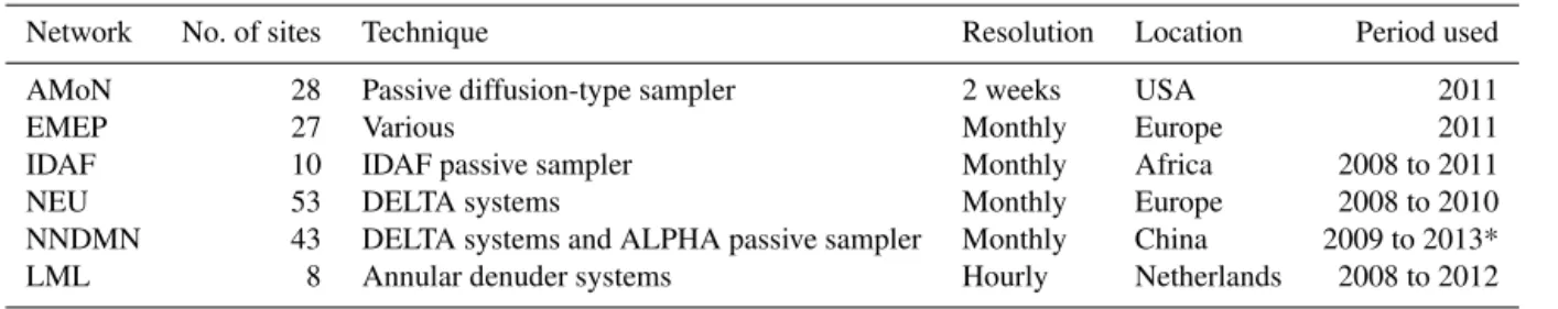
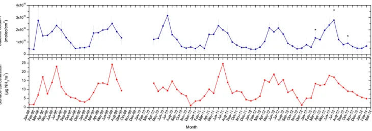
chemi-Figure 1.Vertical distribution of NH3airborne measurements from
the NOAA WP-3D flights during the CalNex campaign in Califor-nia (2010). Each color corresponds to 1 day of measurement.
cal ionization mass spectrometry (CIMS, uncertainty of ±
(30 %+0.2 ppbv)) during 16 flights of the National Oceanic
and Atmospheric Administration (NOAA) WP-3D aircraft (Nowak et al., 2007, 2010, 2012). The observations were made at 1 Hz which is equivalent to 100 m spatial resolution, with the majority of measurements at altitudes from 10 m to 2 km above ground. Nowak et al. (2012) used this data set to show the underestimation of NH3 emissions from dairy
farms and automobiles in regional emissions inventories and to assess the impact of these sources on the formation of am-monium nitrate. Figure 1 presents the high-resolution NH3
profiles from the campaign, with x axis being linear from
0 to 100 pbbv and logarithmic from 100 to 1000 ppbv. The large majority of measurements range from 0 to 100 ppbv, with few measurements reaching as high as several hundred ppbv.
3 Results and discussions
This section starts with a comparison between IASI-NH3
observations and ground-based measurements. A first qual-itative NH3 global comparison is performed for the year
2011, followed by quantitative regional analyses with data sets over Europe, China and Africa. Then the ground-based
hourly measurements provided by the Dutch national net-work (LML) are used to evaluate the IASI measurements col-located in time and to discuss the challenges of validating the satellite measurements of reactive species, showing high spa-tial and temporal variability. The added value of the airplane measurements for validation of IASI-NH3 measurements is
presented in Sect. 3.2.
3.1 Comparison with ground-based observations
3.1.1 Global evaluation
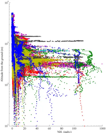
Figure 2 shows the NH3distribution measured by IASI for
2011 and gridded at 0.25◦lat×0.5◦long resolution for the areas covered by the available measurement data sets. In this graphic a weighting procedure has been applied on the IASI daily columns to take into account the error variabil-ity of the data set within the average (Van Damme et al., 2014a). The main agricultural source areas are observed in the Indo-Gangetic plain, the North China Plain (NCP) as well as intensive agricultural valleys such as the Ferghana Val-ley in central Asia and the San Joaquin ValVal-ley in California (Clarisse et al., 2009, 2010). High NH3values are also seen
over burned areas mainly in Eastern Europe (April) (IFFN-GFMC-16, 2011), over the Magadan region in eastern Rus-sia (May and especially second part of July) (NASA, 2011) and in Indonesia (March). Ground-based data sets of NH3
concentrations for 2011 have been superimposed in Fig. 2. What is striking from the collected data sets for that year is the scarcity of the NH3 measurements in some parts of
the world. Except for the IDAF stations in Africa, no mea-surements were available for 2011 in the rest of the trop-ical region and in the Southern Hemisphere. Nevertheless, we find a broadly similar pattern in the surface measurement as in the satellite-derived distribution, with the largest con-centrations for the Chinese stations, followed by the IDAF sites in Africa. Europe and the USA present lower concen-trations with the exception of the Eibergen station (EMEP) in the Netherlands (see also below).
Although the comparison with the IASI measurements is qualitatively reasonable, we find that in North America the satellite-retrieved columns are relatively higher than the ones reported by the AMoN network. It is worth noting that the sites with yearly concentrations available for 2011 are mainly located outside the intensive source areas for the USA. In China, the highest values are observed (from the ground and IASI) in the NCP and in the Chengdu Plain (Sichuan basin). The satellite columns are lower in southeast-ern China, which is consistent with the high-resolution NH3
emissions inventory from Huang et al. (2012). In Europe, the EMEP stations are mainly located in its central part, where IASI-NH3 columns have low values, in agreement with the
Figure 2.Yearly averaged surface concentrations (µg m−3, left vertical color bar) from IDAF, AMoN, EMEP and NNDMN data sets plotted on top of the NH3IASI satellite column (×1016molec cm−2, right vertical color bar) distribution for 2011 gridded at 0.25◦lat×0.5◦long. Columns and relative error (%, bottom left inset) have been calculated as a weighted mean of all IASI measurements within a cell, following equations described in Van Damme et al. (2014a) (columns with an associated relative above 100 % have been filtered).
hotspot in Europe is the Po Valley of northern Italy. Although this was not represented by the EMEP measurements, this is subject of a specific analysis under the ECLAIRE project (eclaire-fp7.eu).
3.1.2 Regional focus
Monthly resolved data sets
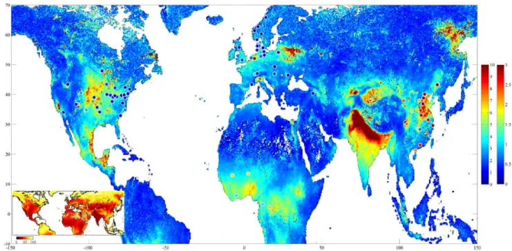
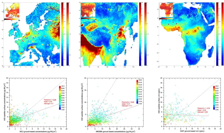
Figure 3 presents a similar comparison with focus over Europe (left), China (middle) and Africa (right). The top panels show the IASI-retrieved column distributions (×1016molec cm−2, right vertical color bar) on which
the ground-based concentrations from the NEU and the NNDMN network (µg m−3, left vertical color bar) and the volume mixing ratio (VMR) from the IDAF network (ppbv, left vertical color bar) have been superimposed. The bottom panels provide the corresponding correlation plots with their linear regression fits (reduced major axis), and Pearson’s cor-relation coefficient (r, underlined when significant). For this
comparison the IASI columns have been converted to sur-face concentrations by using the model profiles considered in the retrieval procedure (Van Damme et al., 2014a). Al-though such a conversion introduces additional errors, it al-lows direct comparison with similar quantities. We note that while the conversion to surface observation does not change the correlation much, it determines the intercept. The use of an inadequate profile shape leads unavoidably to biased sur-face concentrations from IASI. As an example, the Pearson’s
r calculated when comparing IASI total columns and NEU
ground-based concentrations is equal to 0.284, while it is equal to 0.275 when comparing satellite and ground-based surface concentrations.
For Europe, the averaged satellite distribution for 2008, 2009 and 2010 is presented with superimposed the 3-year mean NEU ground-based observations (Fig. 3, top left). High values can in particular be seen in the western part of sia, which is an area that was strongly impacted by the Rus-sian fires of 2010 (R’Honi et al., 2013). The effect of these fires appears to be overrepresented in the satellite distribu-tion due to the weighted averaging procedure associated with the higher IASI sensitivity in fire plumes (Van Damme et al., 2014a, b). However, overall IASI observes a similar pattern as that reported by the NEU sites. The highest surface con-centrations are measured in northwestern Europe, going up to 7 µg m−3at Cabauw, Netherlands, where satellite columns
are above 2×10¹⁶molec cm−2. The lowest surface
indi-Figure 3.Top: ground-based quantities (left vertical color bar) from NEU (µg m−3, left panel), NNDMN (µg m−3, middle panel) and IDAF (ppbv, right panel) data sets plotted on top of the NH3satellite columns (×1016molec cm−2, right vertical color bar) distribution gridded at 0.25◦lat×0.5◦long, both averaged for the period covered by the data sets. Stations with less than two-thirds of measurement availability for the period considered have been excluded. The relative error distribution from IASI retrieval is shown as inset (top left, %, horizontal color bar). Columns/errors have been calculated as a mean of all the measurements within a cell, weighted by the relative error following equations described in Van Damme et al. (2014a). Bottom: monthly NEU (left panel), NNDMN (middle panel) ground-based concentrations (µg m−3) and IDAF (right panel) ground-based VMR (ppbv) vs. IASI-retrieved NH3surface concentrations (µg m−3) or VMR (ppbv). The color scale
corresponds to the IASI retrieval errors (%). Dashed red lines represent the linear regression and gray dashed lines represent the one-to-one line. The Pearson’sr(underlined when significant (pvalue below 0.05)), slope and intercept are also indicated in red.
cated in red and is characterized by a Pearson’srof 0.28 (n=
1337 number of coincidences), a slope of 0.42 and an inter-cept at 2.1 µg m−3. Note that if the satellite data are restricted to the monthly mean concentrations with associated error be-low 75 %, the Pearson’s r increases to 0.35 (n=961).
Al-most all the sites in Europe are characterized by a positive correlation coefficient when it is significant (pvalue below
0.05). The highest correlation (r=0.81) is obtained for the
Fyodorovskoye site (RU-Fyo), and this is explained by the very large columns observed during the Russian fire event of 2010. The second site characterized by a high correlation co-efficient is the Monte Bondone site (IT-MBo) withr=0.71,
which is characterized by high NH3concentrations in
sum-mer and low in winter, consistent with local livestock grazing patterns. By contrast, the most northern sites (located in Fin-land) indicate a negative correlation (Hyytiälä, r= −0.44;
Lompolojänkkä,r= −0.43; Sodankylä,r= −0.45) with an
associated p value slightly above 0.05. These are the sites
with very low ground level concentrations (3-year average
close to 0.1 µg m−3), suggesting that the monthly
variabil-ity for such small concentrations in a region associated with low thermal contrast cannot be reliably detected by IASI. The other NEU stations with a significantr above 0.5
in-clude Brasschaat (BE-Bra, 0.54), Fougères (FR-Fou, 0.58) and Vall d’Alinyà (ES-VDA, 0.58). The list of stations and their respective correlation coefficient, as well as their asso-ciatedpandnvalues, is provided in Table A1.
For China (2009 to 2013), the spatial patterns in NH3
abundance are in good agreement (Fig. 3, top middle panel). We find the highest concentrations in the NCP area and the lowest in remote areas such as the Linzhi site (LZ, on the Tibetan Plateau) and several sites in northeast China. To better illustrate the potential for a high degree of cor-respondence between the satellite columns and the surface measurements, we provide in Fig. 4 the monthly averaged time series at Shangzhuang (SZ) from the ground and from space (r=0.72). This suburban station northwest of
Figure 4.Time series of monthly averaged NH3satellite columns (top, blue, molec cm−2) and ground-based concentrations (bottom, red, µg m−3) at Shangzhuang site (40.14◦N, 116.18◦E) in the North China Plain (NCP) from January 2008 to February 2014. The associated weighted mean error for each month is calculated following equations described in Van Damme et al. (2014a) and presented here as error bars. Asterisks highlight the fertilization peaks of March, July and October 2013 (Shen et al., 2011).
from a main road (Shen et al., 2011), has one of the longest records of NH3concentrations in China, from January 2008
to February 2014. The IASI-derived total columns (top, blue, molec cm−2) reproduce nicely the ground-based concentra-tions (bottom, red, µg m−3) time evolution with concentra-tion peaks in summer (June–July), close to 25 µg m−3at the surface and around 3×10¹⁶molec cm−2observed from IASI.
Looking at interannual variability, for example in 2013, the fertilization peaks of March, July and October are clearly observed (Shen et al., 2011). It is interesting to note that the highest January surface concentration (5.1 µg m−3) and
satellite total column (7.8×10¹⁵molec cm−2) are measured
during the severe winter pollution episode of 2013 (see Boy-nard et al., 2014; Wang et al., 2014). The correlation anal-ysis for the monthly values of the 43 NNDMN sites gives a Pearson’srequal to 0.39 (considering the IASI data with
a monthly relative retrieval error below 100 %) and a slope of the regression equal to 0.21 (n=1149). The Pearson’s
r is globally higher than for Europe probably due to the
higher concentrations in China. This is also observed in the monthly retrieval error which are overall lower. In addition to Shangzhuang, the sites with a significant Pearson’sr above
0.5 are China Agricultural University (CAU, 0.51), Ling-shandao (LSD, 0.55), Changdao (CD, 0.58), Gongzhuling (GZL, 0.52), Bayinbuluke (BYBLK, 0.59), Fengyang (FY, 0.64), Ziyang (ZY, 0.58), Yanting (YT, 0.70) and Dianchi (DC, 0.64), where the p values for these sites are all less
than 0.01. Only one site in the NNDMN network gives a sig-nificant negative correlation: the cleanest site in the network in Tibetan Plateau (LZ, r= −0.75). With a mean
ground-based concentration of 1.03 µg m−3, this again illustrates, as
suggested with the Finnish sites, the limitation of IASI to provide reliable monthly NH3values at very low
concentra-tions. The results for all the sites are presented in Table A2.
For Africa, both IASI and surface network report the high-est values in whigh-estern and central Africa and the lowhigh-est in South Africa for the 4-year average (2008 to 2011, Fig. 3 top right panel). However, over Western Africa the highest VMR are reported by the network for the dry savanna sites (located above 10◦N), while IASI observes higher columns closer to the coast. This could possibly be due to the lack of IASI sampling above these Sahelian sites during the rainy season in June–July, which is characterized by large concen-trations measured at the surface. The high density of live-stock concentrated on the fresh pasture at that time implies high surface emissions. However, this time period is typically also associated with a high deposition and/or cloud coverage, preventing IASI from capturing these events while they are monitored from the ground (Adon et al., 2010). Adon et al. (2010) have shown that the dry savanna sites are character-ized by higher concentrations during the wet season (June– July); conversely, the wet savanna sites (closer to the West African coast) present the larger amount during the dry sea-son (January–February). The latter may therefore be better monitored by IASI. The right bottom plot (Fig. 3) compares the surface VMR for Africa in ppbv. There is no correlation when the data of all the sites are grouped. This could be ex-plained by the sparsity of the IDAF data set combined with the difficulties of the satellite to catch specific high emission events. The only station showing a positive significant Pear-son’sr is Lamto (Ivory Coast, 0.39), which is not
surpris-ingly a wet savanna site. The comparison for each station individually is provided in Table A3.
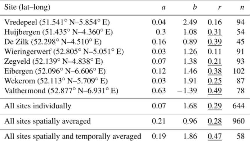
Table 2.Statistical analysis of the comparison of LML and IASI satellite surface concentrations in the Netherlands from 1 January 2008 to 31 December 2012. The spatial averaging (two bottom rows in the table) consists of considering the mean of all the ground-based observations and the mean of the satellite observations in the area covered by the LML network (considered here as the box 51.185–53.022◦N and 4.01– 7.106◦E). The temporal averaging (bottom row) consists in taking the mean of the observations (at the overpass time of the satellite) on a monthly basis. The slope and the intercept of the linear regression are indicated byaandbwhile the significant Pearson’s correlation coefficients (r) are underlined (pvalue below 0.05);ncorresponds to the number of points. Only IASI-derived values with a relative retrieval error below 100 % have been taken into account.
Site (lat–long) a b r n
Vredepeel (51.541◦N–5.854◦E) 0.04 2.49 0.16 94
Huijbergen (51.435◦N–4.360◦E) 0.3 1.08 0.31 54
De Zilk (52.298◦N–4.510◦E) 0.16 0.89 0.39 45
Wieringerwerf (52.805◦N–5.051◦E) 0.03 1.26 0.11 91
Zegveld (52.139◦N–4.838◦E) 0.07 1.38 0.21 93
Eibergen (52.096◦N–6.606◦E) 0.12 1.46 0.38 102
Wekerom (52.113◦N–5.709◦E) 0.03 1.91 0.25 87
Valthermond (52.877◦N–6.931◦E) 0.63 −1.39 0.49 78
All sites individually 0.07 1.68 0.29 644
All sites spatially averaged 0.21 0.96 0.28 960
All sites spatially and temporally averaged 0.19 1.86 0.47 58
in the retrieval procedure for IASI spectra. Indeed, in the case of a low boundary layer height, concentrations are larger in that narrow layer, which is not considered by the straight-forward procedure applied to retrieve IASI surface concen-trations from the columns. Moreover, the vertical profiles above land from the GEOS-Chem model have already been identified as being too low above California, especially for strongly polluted areas (Schiferl et al., 2014). Another rea-son could lie in the influence of very local sources on the ground-based data (see further). Contrary to what we find for high concentrations, there is a positive bias of IASI for low concentrations. There are at least three possible reasons for this. The first stems from the way the relative retrieval er-rors are taken into account. Applying weighted averaging of IASI columns using the relative retrieval error tends to fa-vor the largest concentrations, as the lower values are associ-ated with higher error estimates for the same value of thermal contrast (Van Damme et al., 2014a). A second reason, in the case of very low NH3amounts, is that the random error of the
HRI always translates into a positive contribution of the col-umn (and hence does not average to zero for zero NH3). The
third reason is again linked with a misrepresentation of NH3
vertical distribution. In low NH3abundance cases and/or in
areas where NH3is being deposited, there is no strong
ver-tical gradient near the surface. The use of a polluted profile shape (peaking at the surface) in the retrieval procedure of IASI surface concentrations tends to overestimate the surface contribution of the total columns.
We recall that all regressions shown and discussed in this section are based on weighted monthly IASI-derived NH3
means, with the weight being determined by the relative error of the individual retrieved columns. We also made the
com-parisons with unweighted monthly means and found some-what different parameters for the regression line but an over-all weak impact on the regression coefficients. In over-all cases, the slope remains well below 0.5 and the intercept smaller but still positive.
Hourly resolved data set
The LML data set offers long-term hourly resolved NH3
measurements allowing the investigation of individual IASI observations and testing the effect of averaging different time scales. However, it is worth noting that this network provides measurements in an area (the Netherlands) that is not partic-ularly favorable for infrared remote sensing of surface pol-lution (low thermal contrast and relatively high cloud cover-age). Table 2 summarizes the results from the comparison of the IASI concentrations (columns converted to surface con-centrations as above) to those measured from the ground. The upper part presents the comparison from the linear re-gression for each individual site (slope (a) and intercept (b)
of the linear regression, Pearson’sr (underlined when
sig-nificant) and the number of observations (n)). We took into
account only the IASI measurements covering the stations, which means that the true elliptical footprint is considered and only the observations including the LML site are kept. Six of the sites show significant correlation and for all, ex-cept for one (Valthermond, which has a negative interex-cept and fairly high slope), we find a very low slope (0.03–0.3) but a high intercept between 0.89 µg m−3(De Zilk) and 1.91
Valther-mond (0.49), De Zilk (0.39) and Eibergen (0.38) sites. When all the sites are taken together we obtain a Pearson’s r of
0.29, a slope of 0.07 and an intercept of 1.68 µg m−3. These results, obtained by comparing individual IASI value with ground-based measurement at the overpass time of the satel-lite, could be due, as discussed previously, to the misrepre-sentation of the vertical distribution in the processing of the spectra and the need to consider the boundary layer height.
A factor preventing one from drawing strong conclusions from this comparison is the spatial representativity of the ground-based measurement within the large footprint of the satellite (going from 113 km2 at nadir to around 613 km2 for the highest satellite viewing angles). It means that local sources inside the satellite footprint could have a strong in-fluence on the IASI column values but not be represented in the ground-based data sets due to the high horizontal gradi-ent of NH3concentrations around the source (Fowler et al.,
1998; Sutton et al., 1998; Hertel et al., 2012). Conversely, background concentrations within the IASI pixel will tend to mask single local sources. The representation issue of ground-based measurement stations has already been high-lighted during model performance evaluation (Wichink Kruit et al., 2012). To avoid this uncertainty, which is difficult to as-sess in the validation, we could consider the general rule that the LML network is representative for the entire Netherlands (Nguyen and R. Hoogerbrugge, 2009). For instance, using the eight stations together we can calculate a daily mean concentration of NH3 at the overpass time of the satellite
that we compare with the IASI-weighted mean of the mea-surements inside the area covered by the network (consid-ered here as the following box: 51.185–53.022◦N and 4.01– 7.106◦E). Doing so, we find that the Pearson’srincreases to 0.28, while the slope and the intercept of the linear regression are 0.21 and 0.96 µg m−3, respectively.
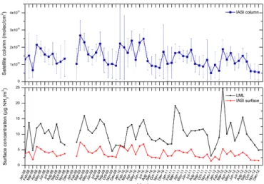
Finally, to investigate the impact of temporal variability and to compare with the previous results of monthly resolved data, we calculated monthly average of IASI measurements above the Netherlands and the LML ground-based concen-trations at the IASI overpass time. The time series of Fig. 5 show the temporal variability in 2008, 2009, 2010, 2011 and 2012 of IASI-NH3 columns (top panel, blue, molec cm−2)
and of the surface concentrations derived from IASI columns (bottom panel, red, µg m−3) and monitored by the LML sites (bottom panel, black, µg m−3). Only values with a relative re-trieval error below 100 % have been taken into account. The spring peak linked with fertilization practices in the Nether-lands is clearly identifiable in the LML and IASI time series in March/April. Looking at the surface concentrations, a fair agreement is found between the ground-based and the satel-lite observations. The monthly variability is consistent be-tween both instruments even if the IASI-derived values are not reproducing with the same amplitude the peaks observed from the ground. This could be due, as explained previously, to a misrepresentation of the NH3 vertical distribution. As
shown in the lowest row of Table 2, the comparison based
Figure 5.Monthly time series of NH3satellite columns (top, blue,
molec cm−2) and surface concentrations at the overpass time of the satellite (bottom) from all the sites of the Dutch LML network av-eraged (black, µg m−3) and from IASI satellite observations (red, µg m−3) (in the box 51.185–53.022◦N and 4.01–7.106◦E, cor-responding to the area covered by the Dutch network), covering 2008, 2009, 2010, 2011 and 2012. The associated error bars are based on the retrieval error for each monthly column, calculated following equations described in Van Damme et al. (2014a). Only monthly means associated with weighted relative retrieval errors be-low 100 % are shown.
on monthly data is characterized by a Pearson’sr of 0.47,
substantially higher than the ones obtained with the previous data sets. The linear regression has a slope of 0.19 and an intercept of 1.86 µg m−3.
3.2 Comparison with airborne observations
California is an important NH3source area in the USA.
Ma-jor sources include livestock operations, agricultural fertil-izers, waste management facilities and motor vehicles (Par-rish, 2014). Figure 6 presents the NH3distributions for the
area and period covered by the CalNex campaign (from 30 April to 24 June 2010). The airborne distribution (top panel, ppbv) is consistent with the satellite one (bottom panel,×1016molec cm−2). The retrieval error distribution is
also presented as inset (bottom left of right panel, %). The pattern observed is characterized by the highest concentra-tions in the San Joaquin and Sacramento valleys, as well as in the South Coast Air Basin (SCAB). High concentrations are also measured in the Imperial Valley and to a lesser ex-tent in the neighborhood of Phoenix. Note that the high val-ues reported by the airborne measurements on 22 June above upper western part of Colorado are also measured by IASI.
Figure 6. NH3 distribution measured from CIMS instrument on-board NOAA WP-3D aircraft (left, ppbv) and IASI satellite (right,
molec cm−2) averaged for the flight period of the CalNex campaign (from 30 April 2010 to 24 June 2010). Averaged relative retrieval
error (%) of the IASI-NH3columns are presented as inset in the lower left corner of right panel. Only column means associated with weighted relative retrieval errors below 100 % are shown.
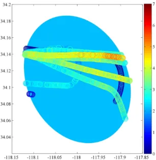
Figure 7.Spatial distribution of 1515 airborne observations made on-board the NOAA WP-3D aircraft at various altitudes superim-posed on the corresponding IASI footprint. The color scale cor-responds to the individual concentrations (ppbv) measured by the CIMS instrument, while the value for IASI is the average of the VMR calculated from the same total column at the different alti-tudes of the aircraft.
then averaged in a second step. This results in 222 corre-sponding pairs of observations to which we can apply thresh-olds on the mistime (being the time difference between the IASI overpass and the airborne measurement), the retrieval error or the number of airborne observations by IASI foot-print.
As an illustration, Fig. 7 shows observations in the SCAB (satellite footprint centered at 34.12◦N and 118◦W) charac-terized by a satellite mean concentration of 2.17 ppbv (asso-ciated with a relative retrieval error of 25 %) and an airborne
Table 3.Statistical analysis of the CalNex and IASI satellite vmr comparison. The slope (a) and the intercept (b) of the linear regres-sions are indicated for various criteria on the data selection, as well as their respective Pearson’s correlation coefficients (r, in italic font when significant);ncorrespond to the number of pairs of observa-tions.
Retrieval error Mistime a b r n
No filter No filter 0.07 2.31 0.36 222
No filter <3 h 0.18 0.64 0.72 75
<100 % <3 h 0.18 0.49 0.82 70
<100 % <1 h 0.17 0.13 0.99 15
concentration of 2.65 ppbv. This subset of observations has been selected as the one with the highest density of airborne measurements for a given IASI footprint (with a relative re-trieval error below 100 %) considering a mistime below 3 h. The IASI footprint in that case includes 1515 individual air-borne observations spanning altitudes from 272 m to 2.6 km. The results obtained from the comparison are presented in Table 3. The first row gives the statistical parameters for all the coupled observations. This comparison is character-ized by a Pearson’sr of 0.36 (n=222), a slope of 0.07 and
an intercept at 2.33 ppbv. Only considering pairs of obser-vations with a mistime of less than 3 h, the Pearson’sr
in-creases significantly to 0.72 (n=75). If a threshold on the
relative retrieval errors is also taken into account (in this case being<100 %), therincreases further to 0.82. Finally, if we
constrain the mistime to be lower than 1 h, the Pearson’sr
reaches 0.99 (n=15). With increased filtering, a decrease of
the intercept is also observed. However, it is notable that the slope of the regression does not change substantially, remain-ing at around 0.17 to 0.18, indicatremain-ing underestimates of NH3
4 Conclusions and perspectives for the validation
Overall, IASI satellite measurements of NH3are consistent
with the available data sets used in this study. This paper presents only the first steps to validate IASI-NH3 columns.
As shown, it is not straightforward and depends strongly on data availability as well as on their representativity for satellite observations. The yearly distributions reveal consis-tent patterns and highlight the scarcity and the spatial het-erogeneity of NH3observations from the ground, with very
few measurements in the Southern Hemisphere and tropical agroecosystems. Comparisons with monthly resolved data sets in Europe, China and Africa have shown that IASI NH3
-derived concentrations are in fair agreement considering that the ground-based observations used here for comparison are mainly monthly integrated measurements, while the satellite monthly weighted means are only taking observations at the morning overpass time into account.
The comparison between IASI-derived concentrations and the surface concentrations measured locally was assessed us-ing linear regressions. Statistically significant correlations were found at several sites, but low slopes and high intercepts were calculated in all cases. Overall, this points to a too-small range in the IASI surface concentrations, which could partly be due to the lack of representativity of the point sur-face measurements in the large IASI pixel. Another possible reason for the difference lies in the use of a simple profile shape in the retrieval procedure, which does not take into account variations in the boundary layer height and hence in the mixing of pollution close to the surface. As shown in previous studies, accounting for realistic boundary layer heights in the retrieval of tropospheric column from satel-lite measurements improves on the comparison with surface measurements (e.g., see Boersma et al., 2009). A third possi-ble contributing reason for the large intercept and low slope is a bias in the IASI values derived from weighted averag-ing, where more weight is given to data with the least uncer-tainty. Under clean conditions, when there is a weak signal, this tends to give more weight to high values, which partly explain the high intercept values.
In addition to the comparison with ground-based mea-surements, this paper has also provided a comparison of the IASI-derived VMR to vertically resolved CIMS measure-ments from the NOAA WP-3D airplane during the CalNex campaign in 2010. The main advantage of such a compar-ison lies in the fact that numerous airborne measurements are available within the satellite footprint, strongly reducing spatial representativity issues. Moreover, airborne measure-ments are performed at altitudes that are more in line with the sensitivity of infrared nadir sounders. Consequently, a much higher correlation between IASI and the airplanes is found, e.g., characterized by a correlation coefficient of 0.82 for sub-set of observations associated with a retrieval error below 100 % for IASI and a mistime below 3 h. Low slopes and large intercept values from the linear regressions are never-theless obtained, as they were with the ground-based mea-surements, further suggesting a poor representativity of the profile shape used for IASI retrievals for these high pollution regions.
More generally, this first attempt to validate the NH3
mea-surements from IASI has highlighted known limitations in both the retrieval procedure (fixed vertical profile and bound-ary layer height) and in the correlative measurements, which are in many cases not representative of what the satellite measures horizontally and vertically. All statistical results were shown for concentrations (or VMR) and do not al-low the validity of the IASI-derived columns to be assessed, which is – considering the limited vertical sensitivity achiev-able – the most relevant quantity availachiev-able from these satel-lite measurements. Therefore, here we highlight the need to acquire more comprehensive data sets of NH3 columns,
e.g., by using boundary layer heights and NH3profile
mea-surements (and/or estimates) to infer the columns abundance from the surface observations. For this purpose, dedicated measurement campaigns focusing on the NH3 vertical
pro-file or additional total column measurements from ground-based Fourier transform infrared, which are becoming avail-able (Vigouroux et al., 2013), will no doubt allow improve-ments in the validation of NH3satellite-retrieved columns in
Appendix A
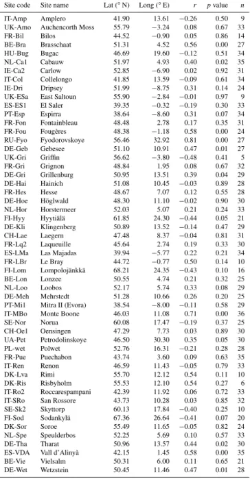
Table A1.Statistical analysis of the NEU data set and monthly IASI satellite surface concentrations comparison for each stations during 2008, 2009 and 2010. Each site is characterized by its site code and name, coordinates, its Pearson’s correlation coefficient (r) and the associatedpvalue as well as its number of points (n). Only monthly values with a relative IASI retrieval errors below 100 % have been taken into account.
Site code Site name Lat (◦N) Long (◦E)
r pvalue n
IT-Amp Amplero 41.90 13.61 −0.26 0.50 9 UK-Amo Auchencorth Moss 55.79 −3.24 0.08 0.67 33
FR-Bil Bilos 44.52 −0.90 0.05 0.86 14 BE-Bra Brasschaat 51.31 4.52 0.56 0.00 27 HU-Bug Bugac 46.69 19.60 −0.12 0.51 34
NL-Ca1 Cabauw 51.97 4.93 0.40 0.02 35 IE-Ca2 Carlow 52.85 −6.90 0.02 0.92 31 IT-Col Collelongo 41.85 13.59 −0.09 0.61 34
IE-Dri Dripsey 51.99 −8.75 0.31 0.14 24 UK-ESa East Saltoun 55.90 −2.84 −0.01 0.97 9 ES-ES1 El Saler 39.35 −0.32 −0.19 0.30 33
PT-Esp Espirra 38.64 −8.60 0.31 0.07 34 FR-Fon Fontainbleau 48.48 2.78 0.17 0.35 31 FR-Fou Fougères 48.38 −1.18 0.58 0.00 24
RU-Fyo Fyodorovskoye 56.46 32.92 0.81 0.00 27 DE-Geb Gebesee 51.10 10.91 0.47 0.01 27 UK-Gri Griffin 56.62 −3.80 −0.48 0.41 5
FR-Gri Grignon 48.84 1.95 0.08 0.67 32 DE-Gri Grillenburg 50.95 13.51 0.39 0.04 29 DE-Hai Hainich 51.08 10.45 −0.03 0.89 28
FR-Hes Hesse 48.67 7.07 0.12 0.55 28 DE-Hoe Höglwald 48.30 11.10 −0.02 0.90 30 NL-Hor Horstermeer 52.03 5.07 0.21 0.24 33 FI-Hyy Hyytiälä 61.85 24.30 −0.44 0.05 21 DE-Kli Klingenberg 50.89 13.52 −0.14 0.47 29 CH-Lae Laegern 47.48 8.37 −0.04 0.81 31 FR-Lq2 Laqueuille 45.64 2.74 0.19 0.33 30 ES-LMa Las Majadas 39.94 −5.77 0.22 0.21 34 FR-LBr Le Bray 44.72 −0.77 0.50 0.14 10 FI-Lom Lompolojänkkä 68.21 24.35 −0.43 0.10 16 BE-Lon Lonzee 50.55 4.74 0.21 0.32 25 NL-Loo Loobos 52.17 5.74 0.33 0.08 29 DE-Meh Mehrstedt 51.28 10.66 0.26 0.20 25 PT-Mi1 Mitra II (Evora) 38.54 −8.00 −0.11 0.58 29 IT-MBo Monte Boone 46.03 11.08 0.71 0.00 36 SE-Nor Norua 60.08 17.47 −0.19 0.37 25 CH-Oe1 Oensingen 47.29 7.73 0.03 0.89 30 UA-Pet Petrodolinskoye 46.50 30.30 0.35 0.05 30 PL-wet Polwet 52.76 16.31 −0.21 0.28 28 FR-Pue Puechabon 43.74 3.60 0.09 0.63 35 IT-Ren Renon 46.59 11.43 −0.05 0.79 33 DK-Lva Rimi 55.70 12.12 0.54 0.11 10 DK-Ris Risbyholm 55.53 12.10 0.54 0.27 6 IT-Ro2 Roccarespampani 42.39 11.92 0.06 0.72 33 IT-SRo San Rossore 43.73 10.28 0.03 0.85 32 SE-Sk2 Skyttorp 60.13 17.84 −0.40 0.25 10 FI-Sod Sodankylä 67.36 26.64 −0.41 0.07 20 DK-Sor Soroe 55.49 11.65 −0.05 0.82 24
NL-Spe Speulderbos 52.25 5.69 0.10 0.57 33 DE-Tha Tharat 50.96 13.57 0.44 0.02 30 ES-VDA Vall d’Alinyà 42.15 1.45 0.58 0.00 35 BE-Vie Vielsalm 50.31 6.00 0.11 0.65 21 DE-Wet Wetzstein 50.45 11.46 0.47 0.01 28
Table A2.Statistical analysis of the NNDMN data set and monthly IASI satellite surface concentrations comparison for each stations during 2009, 2010, 2011, 2012 and 2013. Each site is characterized by its name and coordinates, its Pearson’s correlation coefficient (r) and the associatedpvalue as well as its number of points (n). Only monthly values with a relative IASI retrieval errors below 100 % have been taken into account.
Site Long (◦E) Lat (◦N) r pvalue n
CAU (China Agricultural University) 116.28 40.02 0.51 0.00 45 BNU (Beijing Normal University) 116.37 39.96 0.64 0.17 6
DBW (Dongbeiwang) 116.28 40.05 – – 0
SZ (Shangzhuang) 116.18 40.14 0.72 0.00 45
BD (Baoding) 115.48 38.85 0.27 0.39 12
QZ (Quzhou) 115.02 36.87 0.32 0.03 44
YQ (Yangqu) 112.67 38.06 0.39 0.01 45
LSD (Lingshan Dao) 120.17 35.78 0.55 0.00 32
CD (Changdao) 120.74 37.91 0.58 0.00 37
YC (Yucheng) 116.63 36.92 0.42 0.12 15
ZMD (ZMD) 114.02 33.01 −0.16 0.30 45
ZZ (Zhengzhou) 113.63 34.75 0.38 0.01 43
DL (Dalian) 121.61 38.91 0.43 0.01 40
GZL (Gongzhuling) 124.82 43.50 0.52 0.00 38
LS (Lishu) 124.34 43.31 0.34 0.03 40
WY (Wuyin) 129.25 48.11 0.24 0.54 9
GH (Genhe) 121.52 50.78 −0.36 0.34 9
TFS (Tufeisuo) 87.28 43.56 0.23 0.50 11
SDS (Shengdisuo) 87.34 43.51 0.21 0.53 11
DL (Duolun) 116.49 42.20 0.52 0.29 6
BYBLK (Bayinbuluke) 84.15 43.03 0.59 0.03 14
WW (Wuwei) 102.61 37.96 −0.19 0.25 39
YL (Yangling) 108.08 34.27 0.02 0.89 45
FH (Fenghua) 121.53 29.61 0.30 0.06 38
FZ (Fuzhou) 119.57 26.06 0.02 0.92 38
WX (Wuxue) 115.94 30.07 0.47 0.01 28
BY (Baiyun) 113.27 23.16 −0.23 0.16 41
ZZ (Zhanjiang) 110.33 21.26 0.05 0.74 39
TJ (Taojiang) 112.16 28.52 0.35 0.05 33
FY (Feiyue) 113.20 28.33 0.16 0.36 35
HN (Huinong) 113.24 28.31 0.34 0.05 35
XS (Xishan) 113.18 28.36 0.47 0.00 36
NJ (Nanjing) 118.50 31.52 0.35 0.16 18
FY (Fengyang) 117.53 32.87 0.64 0.03 11
WJ (Wenjiang) 103.86 30.68 0.02 0.92 38
ZY (Ziyang) 104.63 30.13 0.58 0.00 38
YT (Yanting) 105.46 31.27 0.70 0.00 29
JJ (Jiangjin) 106.26 29.29 0.14 0.67 12
YNAU (Yunnannongda) 102.75 25.13 0.42 0.17 12
DC (Dianchi) 102.64 25.00 0.64 0.03 12
KY (Kunyang) 102.73 25.04 0.39 0.21 12
LZ (Linzhi) 94.36 29.65 −0.75 0.00 12
XN (Xining) 101.79 36.62 1.00 1.00 1
Table A3.Statistical analysis of the IDAF data set and monthly IASI satellite surface concentrations comparison for each stations during 2008, 2009, 2010 and 2011. Each site is characterized by its name and coordinates, its Pearson’s correlation coefficient (r) and the associatedp value as well as its number of points (n). Only monthly values with a relative IASI retrieval errors below 100 % have been taken into account.
Site Lat (◦N) Long (◦E)
r pvalue n
Banizoumbou 13.52 2.63 −0.01 0.95 47 Katibougou 12.93 −7.53 0.01 0.95 47
Agoufou 15.33 −1.48 0.06 0.73 35
Lamto 6.22 −5.03 0.39 0.01 40
Djougou 9.65 1.73 −0.04 0.81 42 Zotélé 3.25 11.88 0.22 0.18 36 Bomassa 2.20 16.33 −0.36 0.03 38 Amersfoort −27.07 29.87 0.04 0.84 34 Louis Trischardt −22.99 30.02 −0.15 0.43 31
Acknowledgements. IASI has been developed and built under the responsibility of the “Centre national d’études spatiales” (CNES, France). It is flown on-board the Metop satellites as part of the EUMETSAT Polar System. The IASI L1 data are received through the EUMETCast near real-time data distribution service. The research in Belgium was funded by the F.R.S.-FNRS, the Belgian State Federal Office for Scientific, Technical and Cultural Affairs (Prodex arrangement 4000111403 IASI.FLOW). M. Van Damme is grateful to the “Fonds pour la formation à la recherche dans l’industrie et dans l’agriculture” of Belgium for a PhD grant (Bour-sier FRIA). L. Clarisse and P.-F. Coheur are, respectively, research associate (chercheur qualifié) and senior research associate (maître de recherches) with F.R.S.-FNRS. C. Clerbaux is grateful to CNES for scientific collaboration and financial support. We gratefully acknowledge support from the project “Effects of Climate Change on Air Pollution Impacts and Response Strategies for European Ecosystems” (ÉCLAIRE), funded under the EC 7th Framework Programme (grant agreement no. 282910). Part of this research was supported by the EC under the 7th Framework Programme, for the project “Partnership with China on Space Data (PANDA)”. We also would like to thanks S. Bauduin, J. Hadji-Lazaro and J.-L. Lacour as well as R. van Oss, H. Volten and D. Swart for their helpful advice.
Edited by: M. Van Roozendael
References
Adon, M., Galy-Lacaux, C., Yoboué, V., Delon, C., Lacaux, J. P., Castera, P., Gardrat, E., Pienaar, J., Al Ourabi, H., Laouali, D., Diop, B., Sigha-Nkamdjou, L., Akpo, A., Tathy, J. P., Lavenu, F., and Mougin, E.: Long term measurements of sulfur diox-ide, nitrogen dioxdiox-ide, ammonia, nitric acid and ozone in Africa using passive samplers, Atmos. Chem. Phys., 10, 7467–7487, doi:10.5194/acp-10-7467-2010, 2010.
August, T., Klaes, D., Schlüssel, P., Hultberg, T., Crapeau, M., Arriaga, A., O’Carroll, A., Coppens, D., Munro, R., and Cal-bet, X.: IASI on Metop-A: Operational Level 2 retrievals after five years in orbit, J. Quant. Spectrosc. Ra., 113, 1340–1371, doi:10.1016/j.jqsrt.2012.02.028, 2012.
Bash, J. O., Cooter, E. J., Dennis, R. L., Walker, J. T., and Pleim, J. E.: Evaluation of a regional air-quality model with bidi-rectional NH3 exchange coupled to an agroecosystem model, Biogeosciences, 10, 1635–1645, doi:10.5194/bg-10-1635-2013, 2013.
Behera, S., Sharma, M., Aneja, V., and R., B.: Ammonia in the at-mosphere: a review on emission sources, atmospheric chemistry and deposition on terrestrial bodies., Environ. Sci. Pollut. Res. Int., 20, 8092–131, doi:10.1007/s11356-013-2051-9, 2013. Boersma, K. F., Jacob, D. J., Trainic, M., Rudich, Y., DeSmedt, I.,
Dirksen, R., and Eskes, H. J.: Validation of urban NO2 concen-trations and their diurnal and seasonal variations observed from the SCIAMACHY and OMI sensors using in situ surface mea-surements in Israeli cities, Atmos. Chem. Phys., 9, 3867–3879, doi:10.5194/acp-9-3867-2009, 2009.
Bouwman, A. F., Boumans, L. J. M., and Batjes, N. H.: Estimation of global NH3 volatilization loss from synthetic fertilizers and
animal manure applied to arable lands and grasslands, Global Biogeochem. Cy., 16, 1024, doi:10.1029/2000GB001389, 2002. Boynard, A., Clerbaux, C., Clarisse, L., Safieddine, S., Pommier, M., Van Damme, M., Bauduin, S., Oudot, C., Hadji-Lazaro, J., Hurtmans, D., and Coheur, P.-F.: First simultaneous space mea-surements of atmospheric pollutants in the boundary layer from IASI: A case study in the North China Plain, Geophys. Res. Lett., 41, 645–651, doi:10.1002/2013GL058333, 2014.
Clarisse, L., Clerbaux, C., Dentener, F., Hurtmans, D., and Coheur, P.-F.: Global ammonia distribution derived from infrared satellite observations, Nat. Geosci., 2, 479–483, doi:10.1038/ngeo551, 2009.
Clarisse, L., Shephard, M., Dentener, F., Hurtmans, D., Cady-Pereira, K., Karagulian, F., Van Damme, M., Clerbaux, C., and Coheur, P.-F.: Satellite monitoring of ammonia: A case study of the San Joaquin Valley, J. Geophys. Res., 115, D13302, doi:10.1029/2009JD013291, 2010.
Clerbaux, C., Boynard, A., Clarisse, L., George, M., Hadji-Lazaro, J., Herbin, H., Hurtmans, D., Pommier, M., Razavi, A., Turquety, S., Wespes, C., and Coheur, P.-F.: Monitoring of atmospheric composition using the thermal infrared IASI/MetOp sounder, At-mos. Chem. Phys., 9, 6041–6054, doi:10.5194/acp-9-6041-2009, 2009.
Coheur, P.-F., Clarisse, L., Turquety, S., Hurtmans, D., and Cler-baux, C.: IASI measurements of reactive trace species in biomass burning plumes, Atmos. Chem. Phys., 9, 5655–5667, doi:10.5194/acp-9-5655-2009, 2009.
Dentener, F., Drevet, J., Lamarque, J. F., Bey, I., Eickhout, B., Fiore, A. M., Hauglustaine, D., Horowitz, L. W., Krol, M., Kul-shrestha, U. C., Lawrence, M., Galy-Lacaux, C., Rast, S., Shin-dell, D., Stevenson, D., Van Noije, T., Atherton, C., Bell, N., Bergman, D., Butler, T., Cofala, J., Collins, B., Doherty, R., Ellingsen, K., Galloway, J., Gauss, M., Montanaro, V., Müller, J. F., Pitari, G., Rodriguez, J., Sanderson, M., Solmon, F., Stra-han, S., Schultz, M., Sudo, K., Szopa, S., and Wild, O.: Ni-trogen and sulfur deposition on regional and global scales: A multimodel evaluation, Global Biogeochem. Cy., 20, GB4003, doi:10.1029/2005GB002672, 2006.
EBAS: available at: ebas.nilu.no, lat access: 19 June 2014. EDGAR-Emission Database for Global Atmospheric Research:
Source: EC-JRC/PBL, EDGAR version 4.2., available at: http: //edgar.jrc.ec.europa.eu (last access: 15th October 2012), 2011. EEA-European Environment Agency: Effects of air
pol-lution on European ecosystems: Past and future ex-posure of European freshwater and terrestrial habitats to acidifying and eutrophying air pollutants, available at: http://www.eea.europa.eu/data-and-maps/indicators/ eea-32-ammonia-nh3-emissions-1/assessment-2 (last access: 20 August 2013), 2014.
EMEP: available at: http://www.nilu.no/projects/ccc/onlinedata/ intro.html, last access: 19 June 2014.
Erisman, J. W., Bleeker, A., Galloway, J., and Sutton, M.: Reduced nitrogen in ecology and the environment, Environ. Pollut., 150, 140–149, doi:10.1016/j.envpol.2007.06.033, 2007.
Erisman, J. W., Sutton, M. A., Galloway, J., Klimont, Z., and Wini-warter, W.: How a century of ammonia synthesis changed the world, Nat. Geosci., 1, 636–639, doi:10.1038/ngeo325, 2008. Erisman, J. W., Galloway, J., Seitzinger, S., Bleeker, A., and
its effect on climate change, Curr. Opin. Environ. Sustain., 3, 281–290, doi:10.1016/j.cosust.2011.08.012, 2011.
Erisman, J. W., Galloway, J. N., Seitzinger, S., Bleeker, A., Dise, N. B., Petrescu, A. M. R., Leach, A. M., and de Vries, W.: Consequences of human modification of the global nitro-gen cycle, Philos. Trans. R. Soc. London, Ser. B, 368, 1621, doi:10.1098/rstb.2013.0116, 2013.
Ferm, M.: A Sensitive Diffusional Sampler, IVL rapport, Swedish Environmental Research Institute, 1991.
Fiore, A. M., Naik, V., Spracklen, D. V., Steiner, A., Unger, N., Prather, M., Bergmann, D., Cameron-Smith, P. J., Cionni, I., Collins, W. J., Dalsoren, S., Eyring, V., Folberth, G. A., Ginoux, P., Horowitz, L. W., Josse, B., Lamarque, J.-F., MacKenzie, I. A., Nagashima, T., O’Connor, F. M., Righi, M., Rumbold, S. T., Shindell, D. T., Skeie, R. B., Sudo, K., Szopa, S., Takemura, T., and Zeng, G.: Global air quality and climate, Chem. Soc. Rev., 41, 6663–6683, doi:10.1039/C2CS35095E, 2012.
Flechard, C. R., Nemitz, E., Smith, R. I., Fowler, D., Vermeulen, A. T., Bleeker, A., Erisman, J. W., Simpson, D., Zhang, L., Tang, Y. S., and Sutton, M. A.: Dry deposition of reactive nitrogen to European ecosystems: a comparison of inferential models across the NitroEurope network, Atmos. Chem. Phys., 11, 2703–2728, doi:10.5194/acp-11-2703-2011, 2011.
Flechard, C. R., Massad, R.-S., Loubet, B., Personne, E., Simpson, D., Bash, J. O., Cooter, E. J., Nemitz, E., and Sutton, M. A.: Advances in understanding, models and parameterizations of biosphere-atmosphere ammonia exchange, Biogeosciences, 10, 5183–5225, doi:10.5194/bg-10-5183-2013, 2013.
Fowler, D., Pitcairn, C., Sutton, M., Flechard, C., Loubet, B., Coyle, M., and Munro, R.: The mass budget of atmospheric ammonia in woodland within 1 km of livestock buildings, Environ. Pollut., 102, 343–348, doi:10.1016/S0269-7491(98)80053-5, 1998. Fowler, D., Coyle, M., Skiba, U., Sutton, M. A., Cape, J. N., Reis,
S., Sheppard, L. J., Jenkins, A., Grizzetti, B., Galloway, J. N., Vitousek, P., Leach, A., Bouwman, A. F., Butterbach-Bahl, K., Dentener, F., Stevenson, D., Amann, M., and Voss, M.: The global nitrogen cycle in the twenty-first century, Philos. Trans. R. Soc. London, Ser. B, 368, 1621, doi:10.1098/rstb.2013.0164, 2013.
Galloway, J.: The Global Nitrogen Cycle, in: Treatise on Geo-chemistry, edited by: Holland, H. D. and Turekian, K. K., 557– 583, Pergamon, Oxford, doi:10.1016/B0-08-043751-6/08160-3, 2003a.
Galloway, J., Aber, J., Erisman, J., Seitzinger, S., Howarth, R., Cowling, E., and Cosby, B.: The Nitrogen Cascade, BioScience, 53, 341–356, 2003b.
Galloway, J. N., Townsend, A. R., Erisman, J. W., Bekunda, M., Cai, Z., Freney, J. R., Martinelli, L. A., Seitzinger, S. P., and Sutton, M. A.: Transformation of the Nitrogen Cycle: Recent Trends, Questions, and Potential Solutions, Science, 320, 889– 892, doi:10.1126/science.1136674, 2008.
Gong, L., Lewicki, R., Griffin, R. J., Flynn, J. H., Lefer, B. L., and Tittel, F. K.: Atmospheric ammonia measurements in Houston, TX using an external-cavity quantum cascade laser-based sensor, Atmos. Chem. Phys., 11, 9721–9733, doi:10.5194/acp-11-9721-2011, 2011.
Hauglustaine, D. A., Balkanski, Y., and Schulz, M.: A global model simulation of present and future nitrate aerosols and their direct
radiative forcing of climate, Atmos. Chem. Phys. Discuss., 14, 6863–6949, doi:10.5194/acpd-14-6863-2014, 2014.
Heald, C. L., Collett Jr., J. L., Lee, T., Benedict, K. B., Schwandner, F. M., Li, Y., Clarisse, L., Hurtmans, D. R., Van Damme, M., Clerbaux, C., Coheur, P.-F., Philip, S., Martin, R. V., and Pye, H. O. T.: Atmospheric ammonia and particulate inorganic nitrogen over the United States, Atmos. Chem. Phys., 12, 10295–10312, doi:10.5194/acp-12-10295-2012, 2012.
Hertel, O., Skjøth, C. A., Reis, S., Bleeker, A., Harrison, R. M., Cape, J. N., Fowler, D., Skiba, U., Simpson, D., Jickells, T., Kul-mala, M., Gyldenkærne, S., Sørensen, L. L., Erisman, J. W., and Sutton, M. A.: Governing processes for reactive nitrogen com-pounds in the European atmosphere, Biogeosciences, 9, 4921– 4954, doi:10.5194/bg-9-4921-2012, 2012.
Huang, X., Song, Y., Li, M., Li, J., Huo, Q., Cai, X., Zhu, T., Hu, M., and Zhang, H.: A high-resolution ammonia emis-sion inventory in China, Global Biogeochem. Cy., 26, GB1030, doi:10.1029/2011GB004161, 2012.
IDAF: IGAC/DEBITS/AFRICA, available at: http://idaf.sedoo.fr/ spip.php?rubrique38, last access: 19 June 2014.
IFFN-GFMC-16: Global Fire Monitoring Center, Global Wildland Fire Network Bulletin No. 16, available at: http://www.fire. uni-freiburg.de/GFMCnew/2011/GFMC-Bulletin-02-2011.pdf (last access: 11 April 2014), 2011.
Krupa, S.: Effects of atmospheric ammonia (NH3) on terres-trial vegetation: a review, Environ. Pollut., 124, 179–221, doi:10.1016/S0269-7491(02)00434-7, 2003.
Leen, J. B., Yu, X.-Y., Gupta, M., Baer, D. S., Hubbe, J. M., Kluzek, C. D., Tomlinson, J. M., and Hubbell, M. R.: Fast In Situ Air-borne Measurement of Ammonia Using a Mid-Infrared Off-Axis ICOS Spectrometer, Environ. Sci. Technol., 47, 10446–10453, doi:10.1021/es401134u, 2013.
Liu, X., Duan, L., Mo, J., Du, E., Shen, J., Lu, X., Zhang, Y., Zhou, X., He, C., and Zhang, F.: Nitrogen deposition and its ecological impact in China: An overview, Environ. Pollut., 159, 2251–2264, doi:10.1016/j.envpol.2010.08.002, 2011.
NADP-National Atmospheric Deposition Program: National Atmo-spheric Deposition Program 2011 Annual Summary, NADP Data Report 2012-01, 2012.
NASA: Fires in Eastern Russia, available at: http://earthobservatory. nasa.gov/NaturalHazards/view.php?id=51539 (last access: 1 De-cember 2014), 2011.
Nguyen, P. and R. Hoogerbrugge, F. v. A.: Evaluation of the repre-sentativeness of the Dutch national Air Quality Network, Tech. Rep. Report 680704010/2009, RIVM, 2009.
Norman, M. and Leck, C.: Distribution of marine boundary layer ammonia over the Atlantic and Indian Oceans during the Aerosols99 cruise, J. Geophys. Res.-Atmos., 110, D16302, doi:10.1029/2005JD005866, 2005.
Nowak, J. B., Neuman, J. A., Kozai, K., Huey, L. G., Tanner, D. J., Holloway, J. S., Ryerson, T. B., Frost, G. J., McKeen, S. A., and Fehsenfeld, F. C.: A chemical ionization mass spectrometry tech-nique for airborne measurements of ammonia, J. Geophys. Res.-Atmos., 112, D10S02, doi:10.1029/2006JD007589, 2007. Nowak, J. B., Neuman, J. A., Bahreini, R., Brock, C. A.,