www.atmos-chem-phys.net/16/15247/2016/ doi:10.5194/acp-16-15247-2016
© Author(s) 2016. CC Attribution 3.0 License.
Effects of daily meteorology on the interpretation of space-based
remote sensing of NO
2
Joshua L. Laughner1, Azimeh Zare1, and Ronald C. Cohen1,2
1Department of Chemistry, University of California, Berkeley, Berkeley, CA, USA
2Department of Earth and Planetary Science, University of California, Berkeley, Berkeley, CA, USA
Correspondence to:Ronald C. Cohen ([email protected])
Received: 27 June 2016 – Published in Atmos. Chem. Phys. Discuss.: 12 July 2016 Revised: 21 October 2016 – Accepted: 4 November 2016 – Published: 9 December 2016
Abstract. Retrievals of tropospheric NO2 columns from
UV–visible observations of reflected sunlight require a pri-ori vertical profiles to account for the variation in sensitiv-ity of the observations to NO2 at different altitudes. These
profiles vary in space and time but are usually approximated using models that do not resolve the full details of this varia-tion. Currently, no operational retrieval simulates these a pri-ori profiles at both high spatial and high temporal resolution. Here we examine the additional benefits of daily variations in a priori profiles for retrievals already simulating a priori NO2profiles at sufficiently high spatial resolution to identify
variations of NO2within urban plumes. We show the effects
of introducing daily variation into a priori profiles can be as large as 40 % and 3×10¹⁵molec. cm−2for an individual day and lead to corrections as large as−13 % for a monthly av-erage in a case study of Atlanta, GA, USA. Additionally, we show that NOxemissions estimated from space-based remote sensing using daily, high-spatial-resolution a priori profiles are∼100 % greater than those of a retrieval using spatially coarse a priori profiles, and 26–40 % less than those of a re-trieval using monthly averaged high-spatial-resolution pro-files.
1 Introduction
NOx (=NO+NO2) is an atmospheric trace gas family that
plays an important role in regulating the production of O3
and particulate matter. NOx is emitted into the atmosphere by natural processes (e.g., lightning, biomass burning) and anthropogenic sources, notably combustion. Understanding the contribution of each source is vital to determining the
ef-fectiveness of current and future efforts to improve air qual-ity and to understanding the chemistry of the atmosphere. Studies have utilized satellite observations to constrain NOx emissions from sources such as lightning (e.g., Miyazaki et al., 2014; Beirle et al., 2010; Martin et al., 2007; Schu-mann and Huntrieser, 2007), biomass burning (e.g., Castel-lanos et al., 2014; Mebust and Cohen, 2014, 2013; Miyazaki et al., 2012; Mebust et al., 2011), anthropogenic NOx emis-sions and trends (e.g., Ding et al., 2015; Lamsal et al., 2015; Tong et al., 2015; Huang et al., 2014; Vinken et al., 2014b; Gu et al., 2013; Miyazaki et al., 2012; Russell et al., 2012; Lin et al., 2010; Kim et al., 2009), soil NOxemissions (e.g., Zörner et al., 2016; Vinken et al., 2014a; Hudman et al., 2012), and NOx lifetime (Liu et al., 2016; Lu et al., 2015; de Foy et al., 2014; Valin et al., 2013; Beirle et al., 2011).
The process of retrieving a tropospheric NO2column with
UV–visible spectroscopy from satellites requires three main steps. First, the raw radiances are fit using differential op-tical absorption spectroscopy (DOAS) to yield slant column densities (Richter and Wagner, 2011). Then, the stratospheric NO2signal must be removed (Boersma et al., 2011; Bucsela
et al., 2013). Finally, the tropospheric slant column density (SCD) must be converted to a vertical column density (VCD) by use of an air mass factor (AMF) and Eq. (1). Depend-ing on the specific algorithm, NO2obscured by clouds may
be ignored (producing a visible-only tropospheric NO2
col-umn; e.g., Boersma et al., 2002), corrected by use of an as-sumed ghost column (e.g., Burrows et al., 1999; Koelemeijer and Stammes, 1999), or corrected via the AMF (e.g., Martin et al., 2002). In all cases, the AMF must account for the vary-ing sensitivity of the satellite to NO2 at different altitudes,
vertical profile of NO2is required. Over low-reflectivity
sur-faces, light scattered in the atmosphere is the primary source of radiance at the detector. The probability of back-scattered light penetrating to a given altitude is greater for higher al-titudes; thus there is greater interaction with, and therefore greater sensitivity to, NO2 at higher altitudes (Richter and
Wagner, 2011; Hudson et al., 1995). Because of this, the cor-rect AMF is smaller in locations influenced by surface NOx sources. The relative contribution of errors in the calculated sensitivity and in the a priori profiles of NO2to error in the
fi-nal VCD varies between polluted and clean pixels (Boersma et al., 2004). Previous work (e.g., Russell et al., 2011) has sought to reduce errors in both and highlighted the impor-tance of accurate a priori profiles in urban areas.
VCD= SCD
AMF (1)
A priori NO2profiles are generated using chemical
trans-port models. Previous studies (e.g., Cohan et al., 2006; Wild and Prather, 2006; Valin et al., 2011; Vinken et al., 2014b; Schaap et al., 2015) have demonstrated that these modeled NO2 profiles are strongly dependent on the spatial
resolu-tion of the chemical transport model used. The impact of model spatial resolution on satellite retrievals has been eval-uated through case studies (Valin et al., 2011; Heckel et al., 2011; Yamaji et al., 2014) and through what could be termed “regional” retrievals (Russell et al., 2011; McLinden et al., 2014; Kuhlmann et al., 2015; Lin et al., 2015) that trade com-plete global coverage for improved spatial resolution of the input assumptions. These studies recommend model resolu-tion of<20 km to accurately capture NOx chemistry for a priori profiles. Russell et al. (2011) showed that increasing the spatial resolution of the input NO2profiles produces a
retrieval that more accurately represents contrast in the spa-tial features of NO2plumes, reducing systematic bias by as
much as 30 %. Reducing these biases improves the clarity of the observed urban–rural gradients by providing unique ur-ban and rural profiles, rather than one that averages over both types of locations. McLinden et al. (2014) showed that us-ing 15 km resolution profiles increased the NO2signal of the
Canadian oil sands by∼100 % compared to the Dutch OMI NO2 (DOMINO) and NASA Standard Product (SP)
prod-ucts. They state that this increase corrects a low bias in the retrieved column amounts.
Currently, only the Hong Kong Ozone Monitoring Instru-ment (OMI) retrieval has made use of daily a priori NO2
pro-files at<20 km spatial resolution (Kuhlmann et al., 2015). Their retrieval covered the Pearl River Delta for the pe-riod October 2006 to January 2007. No operational retrieval covering the majority of the OMI data record does so. The current-generation BErkeley High Resolution (BEHR) (Rus-sell et al., 2011, 2012) and OMI-EC (McLinden et al., 2014) retrievals simulate monthly average NO2 profiles at 12 and
15 km, respectively. Conversely, the DOMINOv2 (Boersma et al., 2011), Peking University OMI NO2 (POMINO; Lin
et al., 2015), and DOMINO2_GC (Vinken et al., 2014b) re-trievals simulate daily profiles at 3◦lon×2◦lat (DOMINO)
and 0.667◦ lon×0.5◦ lat (POMINO and DOMINO2_GC),
which is insufficient to capture the full spatial variability of NO2 plumes but does capture large-scale variations in
meteorology. Lamsal et al. (2014) quantitatively compared NO2average profile shapes measured from the P3-B aircraft
for each of six sites in the Deriving Information on Surface conditions from COlumn and VERtically resolved observa-tions relevant to Air Quality (DISCOVER-AQ) Baltimore– Washington D.C. campaign with the modeled profile shape from the Global Modeling Initiative (GMI) chemical trans-port model used to compute the NO2a priori profiles in the
NASA Standard Product v2 retrieval, which uses monthly average NO2 profiles at 2◦×2.5◦ spatial resolution. They
found up to 30 % differences between the measured and mod-eled profile shape factors (i.e., S(p) in Eq. 3) at any sin-gle pressure throughout the troposphere. Several sites (Edge-wood, Essex, and Beltsville) had less NO2 than the model
throughout the free troposphere, and Edgewood also exhib-ited an elevated NO2 layer at 970 hPa not captured in the
model.
Lamsal et al. (2014) also noted that there was signifi-cant day-to-day variability in the measured profiles that can-not be captured by a monthly average model; however, they do not quantify those differences. These day-to-day differ-ences can be significant in a priori NO2profiles. Valin et al.
(2013) showed that the concentration of NO2downwind of a
city increases significantly with wind speed, observing that NO2 100–200 km downwind from Riyadh, Saudi Arabia,
was approximately 130–250 % greater for wind speeds be-tween 6.4–8.3 m s−1 than wind speeds <1.9 m s−1. When
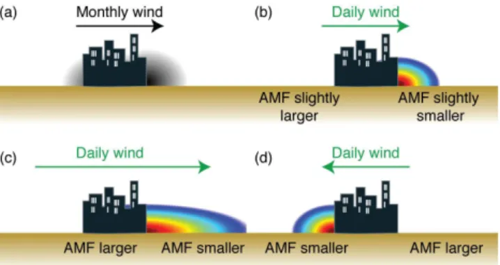
monthly average a priori profiles are used, this is not ac-counted for in the retrieval. The effect on the AMF is illus-trated in Fig. 1c. Compared to the monthly average a priori profiles, daily profiles from a day with fast winds would con-tain greater near-surface NO2further from the city. As
dis-cussed before Eq. (1), UV–visible satellite observations of NO2 are less sensitive to NO2 at low altitudes, so this
re-quires smaller AMFs at a greater distance from the city on days with fast winds to compensate through Eq. (1).
Figure 1.An illustration of the central issues that will be discussed in this paper.(a)The monthly average a priori profiles, shown as the grayscale plumes.(b) A case when the daily wind is similar to the monthly average wind.(c)A case where the daily wind is significantly faster than average but blows in the same direction. (d)A case where the daily wind direction is different than average. The text below each panel describes how the AMF derived from the daily profile would compare with those derived from the monthly a priori.
profile shape resulting from day-to-day variability in wind speed from random to systematic. For example, Beirle et al. (2011), Valin et al. (2013), and Lu et al. (2015) derive an ef-fective NOxlifetime using data with fast wind speed, and Liu et al. (2016) does so by fitting a function with a component derived at slow wind speeds to data derived from days with fast wind speeds. On a day when the wind speed is faster than average, a priori NO2profiles taken from a monthly
av-erage model would have less near-surface NO2further from
the city than is actually present for that day (i.e., Fig. 1c vs. a). The resulting incorrect AMFs would lead to an underes-timation of the spatial extent of the plume and could lead to an underestimate of the NOxlifetime as a consequence.
In this paper, we explore how day-to-day changes in the a priori NO2profiles affect satellite retrievals of urban NO2.
Several scenarios are illustrated in Fig. 1. In each case the change in the AMF results because, over low-albedo sur-faces, a UV–visible satellite spectrometer is less sensitive to near-surface trace gases, necessitating a smaller AMF to ac-count for the reduced sensitivity. In Fig. 1a, the monthly av-erage NO2plume is shown as the grayscale gradient, to
em-phasize that it is static from day to day. Most of the plume follows the prevailing wind direction (here, to the right), but, because days with different wind directions are averaged to-gether, there is some influence of the plume upwind of the city. Figure 1b shows a case where the daily winds are sim-ilar to the monthly average. This leads to a simsim-ilar NO2
plume to the monthly average, but, because we are not aver-aging different wind directions, the upwind plume influence is removed (increasing the AMF, reflecting the reduction in near-surface NO2), and conversely the downwind AMFs are
slightly smaller, due to a slight increase in near-surface NO2
from not averaging in days when the wind direction is
differ-ent. Figure 1c shows a case where the daily winds are faster than the average. Here the AMFs within the city need to be larger, as near-surface NO2is being removed more efficiently
and transported downwind, where the AMFs must therefore be smaller. Finally, Fig. 1d has the wind change direction from the monthly average. Left of the city must have smaller AMFs to account for the presence of the plume not seen in the monthly average, and the opposite change occurs to the right.
We combine the high-spatial-resolution a priori previously developed as part of the BEHR algorithm (Russell et al., 2011) with high temporal resolution to demonstrate the im-pact of day-to-day variations in the modeled NO2profiles on
the calculated AMFs surrounding a major urban area such as Atlanta, GA, USA. Atlanta provides an example of a strong NOxarea source relatively isolated from other sources, with straightforward response of the day-to-day a priori profiles to meteorological variables. Our point is not to derive exact answers for the size and frequency of the effects of daily pro-files, but rather to illustrate that these effects are large enough that their role should be assessed in any future analysis that does attempt to interpret space-based remote sensing of NOx. We show that the variability in the a priori profiles is largely due to changes in wind speed and direction. We first con-sider the effects of day-to-day variations in a priori profiles on AMFs for the region surrounding Atlanta for a fixed grid of OMI pixels, simplifying day-to-day comparisons. We then fully implement 91 days of retrieval to examine the effect on both day-to-day and monthly average NO2columns. Finally,
we apply the exponentially modified Gaussian (EMG) fitting method of Lu et al. (2015) to the new retrieval and show that the spatial and temporal resolution of the a priori profiles can significantly alter the derived emission rate and lifetime.
2 Methods
2.1 The Ozone Monitoring Instrument
pub-licly available global NO2 products, the KNMI DOMINO
product (Boersma et al., 2011) and the NASA Standard Prod-uct (Bucsela et al., 2013).
2.2 BErkeley High Resolution retrieval
The BEHR retrieval is described in detail in Rus-sell et al. (2011), and updates are described on the BEHR website (http://behr.cchem.berkeley.edu/Portals/2/ Changelog.txt). The product is openly available for down-load at http://behr.cchem.berkeley.edu/. Briefly, the BEHR retrieval is based on the NASA SP v2 retrieval (Bucsela et al., 2013; Krotkov and Veefkind, 2006). The total slant column densities (SCDs) are from the OMI NO2 product
(OMNO2A) v1.2.3 (Boersma et al., 2002; Bucsela et al., 2006, 2013) and have been recently evaluated by van Geffen et al. (2015) and Marchenko et al. (2015). The stratospheric subtraction and destriping used is that of the NASA SP v2 retrieval. The tropospheric AMF is then recalculated simi-larly to the AMF formalism described in Palmer et al. (2001). Clear and cloudy AMFs are calculated as shown in Eq. (2). p represents the vertical coordinate as pressure.w(p) rep-resents scattering weights derived from the NASA SP v2 look-up table.g(p) represents the mixing ratio NO2a
pri-ori profile taken from the Weather Research and Forecasting model coupled with Chemistry (WRF-Chem), simulated at 12 km resolution in the published BEHR product.p0
repre-sents the surface pressure (clear-sky AMF) or cloud pressure (cloudy AMF) of the satellite pixel, and ptpthe tropopause
pressure. The cloud pressure is that provided in the NASA SP v2 product and is retrieved using the OMI O2–O2cloud
algorithm (Acarreta et al., 2004; Sneep et al., 2008; Bucsela et al., 2013). A static tropopause pressure of 200 hPa is used. psurfin Eq. (3) is the terrain surface pressure. The integration
is carried out using the scheme described in Ziemke et al. (2001), which allows integration of mixing ratio over pres-sure.
AMF=
ptp Z
p0
w(p)S(p)dp, (2)
where
S(p)=Rptp 1
psurfg(p)dp
g(p). (3)
The scattering weights,w(p), depend on the viewing geom-etry, surface albedo, and terrain pressure altitude. The BEHR algorithm uses the 0.05◦×0.05◦Moderate Resolution Imag-ing Spectroradiometer (MODIS) combined black-sky albedo product (MCD43C3; Schaaf and Wang, 2015) and a surface pressure derived from the Global Land One-km Base Eleva-tion project database (http://www.ngdc.noaa.gov/mgg/topo/ globe.html; Hastings and Dunbar, 1999) with a 7.4 km scale height as inputs to the clear-sky scattering weights. Cloudy
scattering weights treat the cloud pressure as the surface pressure and use an assumed cloud albedo of 0.8 (Stammes et al., 2008; Bucsela et al., 2013). The final AMF is computed as the cloud radiance fraction (frad) weighted average of the
clear and cloudy AMFs (Eq. 4). The cloud radiance fraction is taken from the NASA SP v2 data product (Bucsela et al., 2013).
AMFtotal=fradAMFcloudy+(1−frad)AMFclear (4)
Calculating clear and cloudy AMFs and using the weighted average to compute the final AMF is consis-tent with the OMI algorithm theoretical basis document (Boersma et al., 2002) and yields only the visible NO2
col-umn as the final product; the visible colcol-umn is the value pro-vided in the BEHRColumnAmountNO2Trop field. A scaling factor is provided in the BEHR product for users who wish to include the ghost column. This factor,G, is computed as
G= Vsurf
(1−fgeo)Vsurf+fgeoVcld
(5)
=
Rptp
psurfg(p)dp
(1−fgeo)
Rptp
psurfg(p) dp+fgeo Rptp
pcldg(p)dp
,
whereVsurfandVcld are the modeled vertical column
den-sities above the ground surface and cloud, respectively, and are obtained by integrating the a priori profile above the sur-face or cloud pressure.fgeo is the geometric cloud fraction
included in the NASA SP, which is the OMI O2–O2 cloud
product (Acarreta et al., 2004). This factor is stored in the BEHRGhostFraction field of the BEHR product. Multiply-ing the VCDs stored in BEHRColumnAmountNO2Trop by these values will provide the estimated total (visible+ghost) column.
The results obtained in this work use the visible columns only. The ghost column is not added in for any of the follow-ing results.
2.3 WRF-Chem
Modeled NO2a priori profiles are simulated using the
WRF-Chem model v3.5.1 (Grell et al., 2005). The domain is 81 (east–west) by 73 (north–south) grid cells centered on 84.35◦W, 34.15◦N on a Lambert conformal map projection (approximate edges of the domain are 89.5 to 79.2◦W and
30.3 to 38◦N). Meteorological initial and boundary
ob-tained from the Model for Ozone and Related chemical Trac-ers (MOZART; Emmons et al., 2010). The Regional Atmo-spheric Chemistry Mechanism, version 2 (RACM2; Goliff et al., 2013) and Modal Aerosol Dynamics Model for Eu-rope/Secondary Organic Aerosol Model (MADE/SORGAM) schemes are used to simulate gas-phase and aerosol chem-istry, respectively; the RACM2 scheme is customized to re-flect recent advancements in understanding of alkyl nitrate chemistry using Browne et al. (2014) and Schwantes et al. (2015) as a basis. Lightning NOxemissions were inactive.
The model is run from 27 May to 30 August 2013. Sim-ilar to Browne et al. (2014), the 5-day period 27–31 May is treated as a spin-up period; thus we use 1 June to 30 August as our study time period. Model output is sampled every half hour; the two output files from the same hour (e.g., 19:00 and 19:30 UTC) are averaged to give a single hourly set of profiles. These hourly NO2profiles are used as the a priori
NO2profiles in the BEHR retrieval (Sect. 2.2). To produce
monthly average profiles, each hourly profile is weighted ac-cording to Eq. (6), wherelis the longitude of the profile and h is the hour (in UTC) that WRF calculated the profile for. The weights are clamped to the range [0,1]. These values are used as the weights in a temporal average over the month in question. This weighting scheme gives higher weights to profiles closest to the OMI overpass time around 13:30 local standard time.
wl=1− |13.5−(l/15)−h| (6) wl∈ [0,1]
The weighting scheme in Eq. (6) was chosen over simply using the model output for 13:30 local standard time for each longitude to create smooth transitions between adjoin-ing time zones. This scheme attempts to account for the day-to-day variability in OMI overpass tracks as well as the fact that pixels on the edge of a swath can be observed in two consecutive overpasses at different local times. More detail is given in the Supplement.
A spatial resolution of 12 km is used as the high-spatial-resolution a priori. To determine the effect of coarser spa-tial resolution, the model is also run at 108 km resolution. At 12 km resolution, profiles are spatially matched to OMI pix-els by averaging all profiles that fall within the pixel bounds. At 108 km resolution, the profile closest to the pixel is used. When using daily profiles, they are temporally matched by identifying those closest to the scan time defined in the time field of the NASA SP v2 data product.
2.4 Implementation of daily profiles
Two retrievals are used to study the effects of incorporating daily a priori profiles in the BEHR algorithm. The first is what we term a “pseudo-retrieval”. To create this retrieval, an 11×19 (across×along track) subset of pixels from OMI orbit 47 335 centered on the pixel at 84.2513◦W, 33.7720◦N is used to provide the pixel corners, solar and viewing zenith
and azimuth angles, terrain pressure, and terrain reflectivity. This swath places Atlanta near the nadir view of the OMI instrument (therefore providing pixels with good spatial res-olution) while also remaining outside the row anomaly. This same subset of pixels is used for all days in the pseudo-retrieval. Cloud fractions are set to 0 for all pixels to consider clear-sky AMFs and simplify the pseudo-retrieval. AMFs are calculated for this subset of pixels with WRF-Chem NO2
profiles from 1 June to 30 August 2013 in Eq. (2). This pseudo-retrieval will allow a simplified discussion of the ef-fects of daily a priori profiles by
1. using a fixed set of OMI pixels. Because OMI pixels do not align day to day, using each day’s true pixels makes a day-to-day comparison more difficult to see. In this pseudo-retrieval, that is alleviated.
2. Using a fixed set of OMI pixels also keeps the scatter-ing weights (w(p)in Eq. 2) constant as the parameters that the scattering weights depend on (solar and viewing zenith angles, relative azimuth angles, terrain albedo, and terrain height) are fixed.
3. Setting cloud fractions to 0 ensures that the AMF for ev-ery pixel is calculated with the full a priori profile, rather than just the above-cloud part. Day-to-day variations in cloud fraction also lead to large changes in AMF be-cause the presence of clouds changes both the scattering weights (due to high assumed reflectivity of clouds and smaller effective surface pressure compared to ground) while also obscuring the NO2profile below the cloud.
Essentially, the pseudo-retrieval is an idealized experiment in which we hold all other variables except the a priori profile constant to compute the theoretical magnitude of the effect of using daily a priori profiles on the AMF. It will be used in Sect. 3.1 to demonstrate the effect of incorporating daily a priori profiles. The daily a priori profiles are also imple-mented in the full BEHR retrieval (no longer using a fixed set of pixels or forcing cloud fractions to 0) to determine the impact of including daily a priori profiles on the VCDs in a realistic case. When averaging in time, all pixels are over-sampled to a 0.05◦×0.05◦ grid. The contribution of each
pixel is weighted by the inverse of its area.
2.5 Evaluation of exponentially modified Gaussian fits
Lu et al. (2015) and Valin et al. (2013) used NO2data from
the DOMINO retrieval to study NOxemissions and lifetime from space, accounting for the effects of wind speed vari-ation. To evaluate the impact of the a priori resolution on methods such as these, a similar procedure to fit an expo-nentially modified Gaussian function to NO2 line densities
relative to the model grid; however, thex andy coordinates of the grid do not correspond directly to longitude and lat-itude. Therefore, the wind fields must be transformed from grid-relative to earth-relative (http://www2.mmm.ucar.edu/ wrf/users/FAQ_files/Miscellaneous.html) as
Uearth=Umodel×cos(α)−Vmodel×sin(α), (7)
Vearth=Vmodel×cos(α)+Umodel×sin(α), (8)
where U and V are the longitudinal and latitudinal wind fields, and cos(α)and sin(α) are outputs from WRF as the variables COSALPHA and SINALPHA.
As in Valin et al. (2013), the satellite pixels are rotated so that wind direction (and therefore NO2plumes) for each
day lies along thexaxis. Pixels affected by the row anomaly or with a cloud fraction>20 % are removed. Pixels within 1◦ upwind and 2◦downwind are gridded to 0.05◦×0.05◦,
averaged in time (weighting by the inverse of the pixel area), and integrated across 1◦perpendicular to thexaxis. This
pro-duces line densities, which are a one-dimensional representa-tion of the NO2concentration at various distances downwind
of the city. Three a priori sets are used to create the retrievals used in this section: coarse (108 km) monthly average, fine (12 km) monthly average, and fine (12 km) daily profiles.
We use the form of the EMG function described in Lu et al. (2015) to fit the calculated NO2line densities, after
expand-ing the definition of the cumulative distribution function:
F (x|a, x0, µx, σx, B)= a 2x0
exp µx x0 +
σx2
2x20− x x0
!
(9)
erfc
−√1
2
x
−µx
σx − σx x0
+B,
where erfc is the error function complement, i.e., erfc(x)= 1−erf(x).F (x|a, x0, µx, σx, B)serves as an analytical func-tion that can be fitted to the observed line densities. We find the values ofa,x0,µx,σx, andBthat minimize the sum of squared residuals betweenF (x|a, x0, µx, σx, B)and the line densities, NO2(x):
Resid(a, x0, µx, σx, B)=
X
x
F (x|a, x0, µx, σx, B) (10)
−NO2(x)
2 .
Eq. (10) is minimized using an interior-point algorithm, find-ing the values of a,x0,µx,σx, andB that best fit the line densities. The values of a,x0, µx, σx, and B have physi-cal significance, and so their optimum values yield informa-tion about the NOxemission and chemistry occurring within the plume (Beirle et al., 2011; de Foy et al., 2014; Lu et al., 2015). Specifically,
– a describes the total amount of NO2in the plume
(re-ferred to as the burden).
– x0is the distance the plume travels in one lifetime,τ. It
relates toτ byx0=τ×w, wherewis wind speed.
– uxdescribes the effective center of the emission source. In the Supplement to Beirle et al. (2011), it is repre-sented byX, which is the point at which exponential decay of the NO2plume begins.
– σx is the standard deviation of the Gaussian compo-nent of the EMG function. Lu et al. (2015) terms this a “smoothing length scale,” which describes smoothing of the data due to the spatial resolution and overlap of OMI pixels (Boersma et al., 2011). It can also be thought of as capturing effects of both the spatial extent of emis-sions and the turbulent wind field.
– Bis the background line density.
For each parameter, uncertainty from the fitting process it-self is computed as the 95 % confidence interval calculated using the standard deviation obtained from the fitting pro-cess. This is combined in quadrature with 10 % uncertainty due to across-wind integration distance, 10 % uncertainty due to the choice of wind fields, and 25 % uncertainty from the VCDs, similar to Beirle et al. (2011) and Lu et al. (2015). Technical details of the EMG fitting and uncertainty calcula-tion are given in the Supplement.
3 Results
3.1 Daily variations
Figure 2 shows the average wind and modeled NO2columns
for June 2013 and the AMF values for the pseudo-retrieval around Atlanta, GA, USA. Atlanta was chosen as the focus of this study because it represents a strong NOxsource rela-tively isolated from other equally large sources. This ensures that changes to the a priori profiles on a daily basis can be at-tributed to a local cause. The prevailing wind pattern advects NO2 to the northeast of Atlanta (the location of Atlanta is
marked by the star), as can be seen in the wind field shown in Fig. 2b and the WRF-Chem NO2columns in Fig. 2c. The
av-erage surface wind speed over Atlanta for June is 5.0 m s−1. This distribution of NO2 leads directly to the lower AMFs
-87 -86 -85 -84 -83 -82 32
32.5 33 33.5 34 34.5 35 35.5
AMF
0.7 0.75 0.8 0.85 0.9 0.95 1 1.05 1.1 1.15 1.2
-87 -86 -85 -84 -83 -82 32
32.5 33 33.5 34 34.5 35 35.5
VCD
NO
2
(molec
cm
)
-2
×1015
0 1 2 3 4 5 6 7
-87 -86 -85 -84 -83 -82 32
32.5 33 33.5 34 34.5 35 35.5
-92 -88 -84 -80 -76 -72
24 26 28 30 32 34 36 38
(a) (b)
(c) (d)
Figure 2.Average conditions for June 2013.(a)The red box indicates the part of the SE US being considered.(b)Surface wind directions from the WRF model; average wind speed is 5.0 m s−1(min: 1.7 m s−1; max: 12.7 m s−1).(c)WRF-Chem tropospheric NO2columns. (d)AMFs for the pseudo-retrieval calculated using the average monthly NO2a priori. The direction of the color bar is reversed in(d), as
small AMFs correspond to high modeled VCDs. In all panels, the star (⋆) indicates the position of Atlanta. Longitude and latitude are marked on thexandyaxis, respectively.
average (Fig. 3b) as the wind direction advects NO2into an
area with low NO2in the monthly average.
Figure 3c shows that the greater near-surface NO2to the
northwest results in lower AMFs than average (blue), while the opposite is true to the east (red). The greater near-surface NO2in profiles to the northwest weightsS(p)in Eq. (2) more
heavily towards lower altitudes, wherew(p)is less, thus de-creasing the overall AMF by∼15 %. The increase in AMFs to the east reflects the inflow of cleaner air from the shift in winds. This reduces near-surface NO2 and increases the
weight of higher altitudes ofS(p), increasing the AMFs by
∼10–35 % (the color bar saturates at±25 % to make the de-crease to the northwest easier to see).
Wind speed also plays an important role in determining the a priori profile shape through transport and chemistry. Fig-ure 3d–f shows results from 18 June, when the wind speed over Atlanta averaged 9.1 m s−1. This results in faster
advec-tion away from emission sources, with 10–15 % increases in modeled NO2columns to the west as the plume is driven east
more strongly. The greatest decreases in AMF (and thus in-creases in VCD) are as much as−13 % and occur between 84 and 83◦W where the increased wind speed has advected the NO2 plume farther than the average. There is also a 2–
13 % increase along the west edge of Atlanta, resulting from the shift of the plume center east.
When the change in AMF from using the daily a priori profiles is averaged over the full time period studied (1 June–
30 August), the percent change in AMF is on average+3.6 % throughout the domain, with a maximum of+9.8 %. All pix-els show a positive change. This occurs because 77 % of the daily profiles have less NO2than the corresponding monthly
average profile, as most pixels will be upwind from the city on any given day and will see a decrease in NO2when
up-wind and downup-wind days are no longer averaged together. This reduces the denominator in Eq. (3) and increases the contribution of upper-tropospheric scattering weights to the AMF. Scattering weights increase with altitude; therefore, this results in a systematic increase of the AMF throughout the domain for the pseudo-retrieval.
-85 -84 -83 -82 33.4 33.6 33.8 34 34.2 34.4 34.6 34.8 35 % ∆ AMF -25 -20 -15 -10 -5 0 5 10 15 20 25 Atlanta
-86.5 -86 -85.5 -85 -84.5 -84 -83.5 33 33.2 33.4 33.6 33.8 34 34.2 34.4 34.6 34.8 35 % ∆ AMF -25 -20 -15 -10 -5 0 5 10 15 20 25 Atlanta
-85 -84 -83 -82
33.4 33.6 33.8 34 34.2 34.4 34.6 34.8 35 % ∆ VCD NO 2 -100 -80 -60 -40 -20 0 20 40 60 80 100
-86.5 -86 -85.5 -85 -84.5 -84 -83.5 33 33.2 33.4 33.6 33.8 34 34.2 34.4 34.6 34.8 35 % ∆ VCD NO 2 -150 -100 -50 0 50 100 150
-85 -84 -83 -82
33.4 33.6 33.8 34 34.2 34.4 34.6 34.8 35 VCD NO 2 (molec. cm -2) ×1015
0 1 2 3 4 5 6 7
-86.5 -86 -85.5 -85 -84.5 -84 -83.5 33 33.2 33.4 33.6 33.8 34 34.2 34.4 34.6 34.8 35 Daily VCD NO 2 (molec. cm -2)
×1015
0 1 2 3 4 5 6 7 (a) (b) (c) (d) (e) (f)
Figure 3.Results from 22 June(a–c)and 18 June(d–f).(a, d)WRF-Chem tropospheric NO2columns for 19:00 UTC.(b, e)The percent
difference in WRF-Chem tropospheric NO2columns at 19:00 UTC for that day vs. the monthly average.(c, f)Percent difference in AMFs using hybrid daily profiles vs. the monthly average profiles in the pseudo-retrieval. In all panels, the star (⋆) indicates the position of Atlanta, and the wind direction around Atlanta is shown by the arrow in the lower four panels. Longitude and latitude are marked on thexandyaxis, respectively.
did not include lightning NOx, so this should be considered a lower bound for the effect of day-to-day changes in the free troposphere. The detailed comparison is described in the Supplement.
3.2 Effects on retrieved vertical column densities in full retrieval
To determine the effect the inclusion of daily a priori pro-files has on the final retrieved VCDs, the daily propro-files were implemented in the full BEHR retrieval. Effects on indi-vidual days and multi-month average VCDs are presented here. The cities of Birmingham, AL, USA, and Montgomery, AL, USA, are included to demonstrate that this effect is significant for cities of various sizes. Atlanta, GA, USA, is the largest, with approximately 5.7 million people, fol-lowed by Birmingham, AL, USA, with 1.1 million and
Mont-gomery, AL, USA, with 374 000 (United States Census Bu-reau, 2015).
Table 1.Statistics on the frequency and magnitude of changes in the retrieved VCDs using a daily vs. monthly average profile for pixels with centers within 50 km of Atlanta, GA, USA (84.39◦W, 33.775◦N); Birmingham, AL, USA (86.80◦W, 33.52◦N); and Montgomery, AL, USA (86.30◦W, 32.37◦N). The “percent of days” values are calculated as the number of days with at least one pixel in that subset with a change greater than the given uncertainty divided by the number of days with at least one pixel unobscured by clouds or the row anomaly. The uncertainty represented byPiσi
1/2
is the quadrature sum of uncertainties from spectral fitting (0.7×10¹⁵molec. cm−2; Boersma et al., 2007, 2011), stratospheric separation (0.2×10¹⁵molec. cm−2; Bucsela et al., 2013), and AMF calculation (20 %; Bucsela et al., 2013).
Percent of days with Percent of days with Min change Max change
1VCD>1×10¹⁵molec. cm−2 1VCD>P
iσi1/2 (molec. cm−2) (molec. cm−2)
Atlanta 39 % 23 % −2.4×10¹⁵ +2.5×10¹⁵ Birmingham 54 % 43 % −3.8×10¹⁵ +3.9×10¹⁵ Montgomery 27 % 20 % −2.2×10¹⁵ +1.9×10¹⁵
-87 -86 -85 -84 -83 -82
32 32.5 33 33.5 34 34.5 35 35.5
% difference (daily prof. - monthly prof.)
-12 -9 -6 -3 0 3 6 9 12 Atlanta
Birmingham Montgomery
-87 -86 -85 -84 -83 -82
32 32.5 33 33.5 34 34.5 35 35.5
NO
emissions
(mol
km
h
)
-2
-1
0 20 40 60 80 100 120
Atlanta Birmingham Montgomery
(a) (b)
Figure 4. (a)24 h average NO emissions from WRF-Chem at 12 km resolution.(b)The change in retrieved VCDs averaged over 1 June to 30 August. Pixels with a cloud fraction>20 % or that are affected by the row anomaly are excluded from the average. Longitude and latitude are marked on thexandyaxis, respectively, for both panels.
NO2plume may only fall within a small number of pixels.
Up to 54 % of days exhibit changes in the VCDs greater than 1×10¹⁵molec. cm−2, and up to 43 % exhibit changes greater than the quadrature sum of uncertainties. This indicates that, when considering individual daily measurements, a consider-able fraction of days with any valid pixels would have biases in the retrieved VCDs above the uncertainty due to the tem-poral resolution of the a priori NO2profiles.
For both significance criteria, Table 1 also indicates that Birmingham and its surrounding area exhibit the largest and most frequent changes when using daily a priori profiles. Figure 4a shows the NO emissions throughout this domain. Birmingham has the second-largest NOx emission rate, af-ter Atlanta, while Montgomery has the smallest of the three cities considered. We note that the largest changes are not as-sociated with the city with the greatest NOxemissions. Both Atlanta and Birmingham fall entirely within the NOx sup-pressed regime in the model, so the larger changes in Birm-ingham are not because NOx chemistry transitions between the NOx suppressed and NOx limited regimes. Instead, the magnitude of these changes is due to Birmingham’s inter-mediate size, where significant NO2is present but emission
occurs over a small enough area that changes in wind di-rection can significantly affect NO2concentration at a short
distance from the source. When considering changes to be
significant if they exceed 1×10¹⁵molec. cm−2, Montgomery
has the least frequent significant changes because it has the smallest VCDs, so a change to the AMF needs to be rather large to produce a significant change in the VCD by this met-ric, since the AMF is a multiplicative factor. When consid-ering the quadrature sum of errors as the significance crite-rion, Montgomery and Atlanta both demonstrate significant changes∼20 % of the time.
Implementing the daily profiles also changes the average VCDs, in addition to the day-to-day changes in VCDs dis-cussed above. Figure 4b shows the changes in VCDs aver-aged over the period studied. The largest decrease around Atlanta is to the northeast, along the direction in which the monthly average model results placed the NO2 plume, but
clear decreases can also be seen to the northwest and south-west. In these directions, a systematic decrease of up to 8 % (4×10¹⁴molec. cm−2) is observed. Although this change is small, it is expected to be systematic. Statistically, a pixel’s a priori profile is more likely to have less surface NO2when
different wind directions are no longer averaged in; thus de-creases in the VCD when using a daily a priori profile are more common.
Greater relative changes are observed around the smaller cities of Birmingham (down to −12.9 %, 5×
10−14molec. cm−2). This appears to be primarily because
the areas of emissions are smaller, which makes shifts in wind direction have a greater average relative effect on the plume shape.
We also compare this average change to the measure-ment uncertainty. The uncertainty due to random errors in the retrieval should reduce as the square root of the number of observations, but delineating random and systematic er-rors in the retrieval is challenging (Boersma et al., 2004). The most optimistic approach assumes that the global av-erage uncertainty of 1×10¹⁵molec. cm−2 (Bucsela et al., 2013) can be treated entirely as random error and can be reduced by √40 for the number of observations (not im-pacted by clouds or the row anomaly), to a lower bound of ∼1.6×10¹⁴molec. cm−2. Most of the changes near the
three cities exceed this lower limit. More realistically, the spectral fitting and stratospheric uncertainty may be consid-ered largely random, but only part of the error in the AMF calculation is random, due to spatial or temporal autocorre-lation in the models or ancillary products (Boersma et al., 2004). For simplicity, we assume that the spectral fitting and stratospheric subtraction errors are entirely random, while only half of the error in the AMF is random. This reduces the error from p(0.7×10¹⁵)2
+(0.2×10¹⁵)2
+(20 %)2
to p(0.11×10¹⁵)2
+(0.03×10¹⁵)2
+(11.6 %)2. Only the
largest changes near Birmingham and Montgomery exceed this threshold. This more conservative estimate suggests that the changes in averages are primarily important for smaller or very geographically concentrated cities, where wind direc-tion can have a large effect. Nevertheless, larger cities may exhibit important changes as well.
Unlike the pseudo-retrieval, where we only allowed the a priori profiles to vary day to day and clouds were set to 0, there is a some spatial structure to these average changes. This is primarily a statistical phenomenon. We use only pix-els with cloud fraction<20 %, which reduces the number of pixels in the average. Within this subset, the wind blows to the southeast out of Atlanta more frequently than other di-rections, so the increases due to properly accounting for the presence of surface NO2average with the more typical
de-creases to give a small average change. The other directions exhibit the expected average decrease in VCDs due to the average increase in AMFs discussed in Sect. 3.1. We expect that over longer periods of time all directions would see a 2–6 % decrease in the average VCDs.
4 Discussion
4.1 Importance of model uncertainty
WRF-Chem has generally been found to reproduce wind fields, especially above 2 m s−1(Tie et al., 2007; Zhang et al., 2009), and spatial variability of trace gases (Follette-Cook et al., 2015) well. Nevertheless, a natural concern when
mod-eling daily NO2profiles for satellite retrievals is the accuracy
of the plume location. We, however, note that the transition from monthly average to daily profiles does not necessarily result in increased model uncertainty, but rather a change in the type of uncertainty.
When using monthly average profiles, the uncertainty in the modeled NO2concentrations compared to the true mean
will be reduced (assuming at least some component of the error is random in nature), but the true day-to-day variabil-ity not captured by the monthly average effectively becomes a new error term. In contrast, when using daily profiles, the random model error is not reduced, but the day-to-day vari-ability is also not averaged out. Ideally, the error in a set of daily profiles will manifest as deviation from the true set of profiles for that day, rather than the monthly profiles’ smaller deviation from a mean set of profiles that itself may not rep-resent any single day.
An important step in managing the uncertainty in the daily profiles is to constrain the modeled meteorology with ob-servations or reanalysis datasets. By default, meteorology in WRF is constrained via initial and boundary conditions only. With larger domains and longer runs, further constraints us-ing four-dimensional data assimilation (FDDA; Liu et al., 2006) and/or objective analysis (Follette-Cook et al., 2015; Wang et al., 2014; Yegorova et al., 2011), possibly combined with periodic model reinitialization (Otte, 2008), are strongly recommended.
4.2 Effects on space-based lifetime and emissions constraints
Recently several authors have used wind-sorted satellite NO2
observations to probe NOx chemistry and emissions from space (Beirle et al., 2011; Valin et al., 2013; de Foy et al., 2014; Lu et al., 2015; Liu et al., 2016). We apply the EMG fit-ting method of Lu et al. (2015) to NO2line densities derived
from NO2columns retrieved using the daily and monthly
av-erage a priori profiles, as well as a monthly avav-erage profile simulated at 108 km resolution, for both Atlanta and Birm-ingham. To match the method of Lu et al. (2015) as closely as possible, we use 3 m s−1as the division between slow and fast winds.
We acknowledge that a 91-day averaging period is signif-icantly shorter than those used in Beirle et al. (2011), Valin et al. (2013), or Lu et al. (2015) (5 years, summer half-year for 7 years, and summer half-year for 3 year periods, respec-tively). However, since the goal of this section is to compare the results obtained using three different sets of a priori pro-files with all other variables equal, we believe that 91 days is sufficient for this purpose.
Additionally, we do not include days around Atlanta on which the wind blows towards the southeast (specifically 0 to
−112.5◦; 0◦is defined as east; negative values are clockwise from east). Significant suburban NO2columns near 83.5◦W,
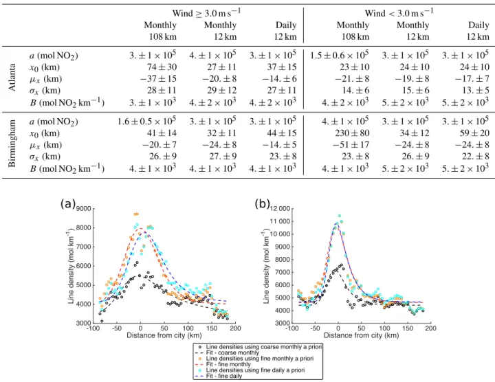
Table 2.Values of the five fitting parameters for the EMG functions (Eq. 9) used to fit the distributions of line densities around Atlanta and Birmingham.arepresents the total NO2burden,x0is the distance the plume travels in one lifetime,µxis the center of emissions relative to the city center,σxdescribes the Gaussian smoothing, andBis the background line density.
Wind≥3.0 m s−1 Wind<3.0 m s−1
Monthly Monthly Daily Monthly Monthly Daily 108 km 12 km 12 km 108 km 12 km 12 km
Atlanta
a(mol NO2) 3.±1×10⁵ 4.±1×10⁵ 3.±1×10⁵ 1.5±0.6×10⁵ 3.±1×10⁵ 3.±1×105
x0(km) 74±30 27±11 37±15 23±10 24±10 24±10
µx(km) −37±15 −20.±8 −14.±6 −21.±8 −19.±8 −17.±7
σx(km) 28±11 29±12 27±11 14.±6 15.±6 13.±5
B(mol NO2km−1) 3.±1×10³ 4.±2×10³ 4.±2×10³ 4.±2×10³ 5.±2×10³ 5.±2×10³
Birmingham
a(mol NO2) 1.6±0.5×10⁵ 3.±1×10⁵ 3.±1×10⁵ 4.±1×10⁵ 3.±1×10⁵ 3.±1×105
x0(km) 41±14 32±11 44±15 230±80 34±12 59±20
µx(km) −20.±7 −24.±8 −14.±5 −51±17 −24.±8 −24.±8
σx(km) 26.±9 27.±9 23.±8 23.±8 26.±9 22.±8
B(mol NO2km−1) 4.±1×10³ 4.±1×10³ 4.±1×10³ 4.±1×10³ 5.±2×10³ 5.±2×10³
Distance from city (km)
-100 -50 0 50 100 150 200
Line density
(mol km
-1 )
3000 4000 5000 6000 7000 8000 9000 10 000 11 000 12 000
Distance from city (km)
-100 -50 0 50 100 150 200
Line density
(mol km
-1)
3000 4000 5000 6000 7000 8000 9000
Line densities using coarse monthly a priori Fit - coarse monthly
Line densities using fine monthly a priori Fit - fine monthly
Line densities using fine daily a priori Fit - fine daily
(a)
(b)
Figure 5.Line densities around Atlanta, GA, USA, averaged over the study period when using monthly average and daily a priori (open circles), and the corresponding fits of exponentially modified Gaussian functions (dashed lines). Black series are derived from a retrieval using a monthly average a priori at 108 km resolution, red series from a monthly average a priori at 12 km resolution, and blue from the daily profiles at 12 km resolution.(a)Average of days with wind speed≥3.0 m s−1.(b)Average of days with wind speed<3.0 m s−1.
can erroneously lengthen the decay time of the fit. All wind directions are used for Birmingham.
Accounting for the spatial and temporal variability of NO2
in the a priori profiles leads to several notable changes in the line densities and the resulting EMG fits. Figure 5 shows the line densities and the corresponding EMG fits around Atlanta for the average over the 91-day study period. Table 2 enumer-ates the values obtained for the fitting parameters in Eq. (9) for the fits of the Atlanta NO2plume in Fig. 5 and fits for the
Birmingham NO2plume (not shown).
The spatial scale of the a priori makes the greatest dif-ference to the maximum value of the line density, causing a significant increase ina when the spatial resolution of the a priori profiles increases from 108 to 12 km. This reflects the
impact of the blurring of urban and rural profiles described in Russell et al. (2011).
Both the spatial and temporal resolution impact the deter-mination ofx0, the distance traveled in one lifetime. This
parameter is determined at fast wind speeds (Lu et al., 2015; Valin et al., 2013), so we consider only the results for wind speed ≥3.0 m s−1. For Atlanta, using a daily a priori re-sults in an x0 value 37 % greater than that obtained
us-ing a monthly average profile at the same spatial resolution (12 km). Birmingham also shows a 38 % increase inx0
be-tween the monthly and daily 12 km a priori.
µxrepresents the apparent center of the NO2plume
ability of the daily a priori to capture how the wind distorts the plume shape.
σx is the Gaussian smoothing length scale, representing both the width of the upwind Gaussian plume and smoothing of the NO2signal due to the physical extent of the source,
the averaging of NO2within one OMI pixel, and daily
vari-ability in the overpass track (Beirle et al., 2011). There is a slight decrease when going from a monthly average to daily profiles, which reflects the general increase in upwind AMFs (i.e., compare Fig. 1a and b), but, because this is outside of the main NO2plume, the effect is small.
Finally,Bis the background line density. Ideally, it is de-rived sufficiently far from any NOxsources that spatial and temporal variability should be minimal. In several cases there is a∼25 % increase when improving the spatial resolution of the a priori profiles. This is likely attributable to the general increase in urban signal discussed several times so far pulling the edges of the line density upward. However, a greater se-lection of cities is necessary to demonstrate this more con-clusively.
Ultimately, the goal of this method is to extract informa-tion about chemically relevant quantities such as emission rate and lifetime. Since de Foy et al. (2014) and Valin et al. (2013) showed that choice of wind speed bins affects the val-ues obtained, we also consider whether the effect of imple-menting the daily a priori profile changes if the observations are binned by different wind speed criteria. Table 3 compares the values of the NOx emission rate,E, and effective life-time,τeff, derived from different wind speed bins for Atlanta
and Birmingham. Restricting the analysis to days with wind speed greater than 5 m s−1results in too few days for a
mean-ingful analysis around Atlanta (due to the need to remove days with winds to the southeast), so results for Atlanta are restricted to≥3 and≥4 m s−1only.
τeff andE are each computed from several of the EMG
fitting parameters.τeffdepends onx0andw(the mean wind
speed) through Eq. (11): τeff=
x0
w. (11)
Edepends ona,x0, andwthrough Eq. (12):
E=1.32×a×w
x0 =
1.32× a
τeff
, (12)
where the factor of 1.32 accounts for the NOx: NO2 ratio
throughout the tropospheric column (Beirle et al., 2011). Both Valin et al. (2013) and de Foy et al. (2014) show that lifetime should decrease at faster wind speeds. We see this trend clearly for Birmingham but not Atlanta. de Foy et al. (2014) also saw that, for a chemical lifetime of 1 h, greater derived emissions were found at faster wind speeds. This is also better seen in our results for Birmingham than Atlanta. Previous measurements of NOxlifetime in urban plumes av-erage 3.8 h and range from 2 to 6 h (Beirle et al., 2011; Ia-longo et al., 2014; Nunnermacker et al., 1998; Spicer, 1982),
and, using the EMG method, Lu et al. (2015) saw effective lifetimes between 1.2 and 6.8 h. The lifetimes we calculate are at the low end of the previously observed ranges. How-ever, this is similar to the instantaneous lifetime of 1.2±0.5 h and 0.8±0.4 h calculated from the WRF-Chem model for days in June 2013 with wind speed≥3 m s−1and grid cells within 50 km of Atlanta and Birmingham, respectively (see the Supplement for the calculation details). The sole excep-tion is the lifetime calculated for Atlanta using the coarse monthly profiles with all wind speeds≥3 m s−1. However, several points near the peak of the line densities for this case are abnormally low compared to their neighbors. This results from the inclusion of negative VCDs in the average to avoid biasing the data; if negative VCDs are not included, the life-time is instead 1.58 h. We expect that with studies expanded over longer time periods the impact of negative VCDs will be reduced.
The differences in the lifetimes and emissions derived us-ing the daily and monthly 12 km a priori profiles are system-atic. In all cases, the lifetime derived using the daily pro-files is 30–66 % longer. When using monthly average a pri-ori profiles, profiles resulting from different wind directions are averaged together. The AMFs calculated from these pro-files thus reflect the average distance from the city the plume reaches in a given direction, e.g., east of the city, with smaller AMFs near the city and greater AMFs being more distant (Fig. 1). In this hypothetical example, when the wind blows to the east, the spatial extent of the plume is underestimated because the average AMFs towards the end of the plume will be too large, so the VCDs will be too small by Eq. (1). On days when the wind does not blow east, the reverse is true: the plume extent is overestimated because the AMFs nearer to the city are too small (Fig. 1d). If one considers a simple average change in the VCDs, these two errors will partially cancel and we will see the average change from Sect. 3.2. However, in the EMG fitting approach, these errors do not cancel at all because the EMG method both rotates the NO2
plumes so that the wind directions align before calculating the line densities and systematically selects fast winds to de-termineτeff, so we are always dealing with the first case and
the plume extent is always underestimated. In the EMG fit, this manifests as a too-short lifetime. As the emissions are inversely proportional to lifetime (Eq. 12), emissions derived using the monthly 12 km a priori profiles will be too great. Therefore, when using a retrieval with a priori profiles at fine spatial resolution, daily temporal resolution of the a priori profiles is necessary to prevent underestimating the lifetime. Further, the spatial resolution of the a priori profiles has a large impact on the magnitude of the derived emissions. To reduce the systematic biases in emissions and lifetime from the choice of a priori profile, it is necessary to simulate these profiles at fine spatial and daily temporal resolution.
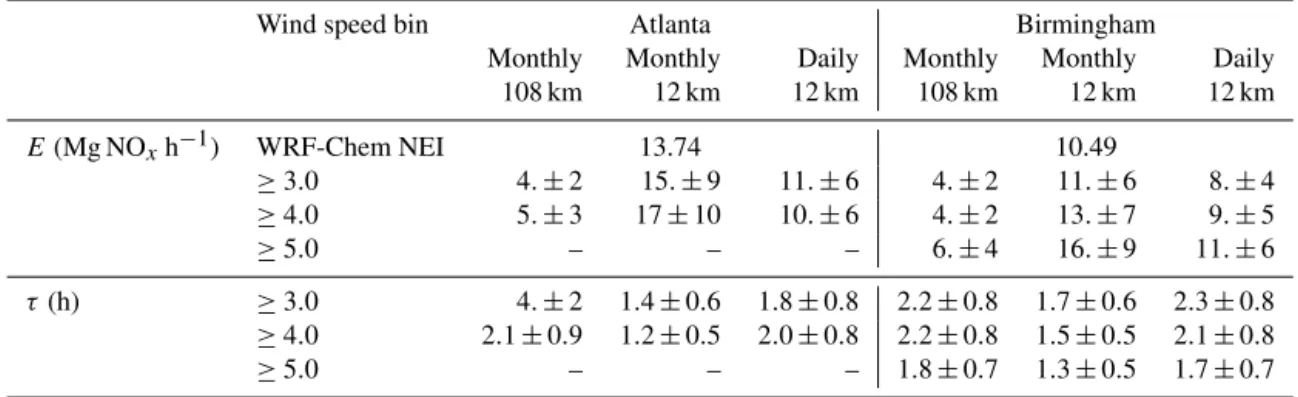
Table 3.Values of the emission rates (E) and effective lifetime (τ) obtained when the separation between slow and fast winds is set at 3, 4, and 5 m s−1. For comparison, the total NOxemission for all 12 km WRF-Chem grid cells within 50 km of each city is given. These emissions are derived from NEI 11 and scaled to 88.9 % to account for 2011–2013 reductions. Uncertainties calculated as described in the Supplement.
Wind speed bin Atlanta Birmingham
Monthly Monthly Daily Monthly Monthly Daily 108 km 12 km 12 km 108 km 12 km 12 km
E(Mg NOxh−1) WRF-Chem NEI 13.74 10.49
≥3.0 4.±2 15.±9 11.±6 4.±2 11.±6 8.±4
≥4.0 5.±3 17±10 10.±6 4.±2 13.±7 9.±5
≥5.0 – – – 6.±4 16.±9 11.±6
τ(h) ≥3.0 4.±2 1.4±0.6 1.8±0.8 2.2±0.8 1.7±0.6 2.3±0.8
≥4.0 2.1±0.9 1.2±0.5 2.0±0.8 2.2±0.8 1.5±0.5 2.1±0.8
≥5.0 – – – 1.8±0.7 1.3±0.5 1.7±0.7
the results derived from using the three different a priori pro-file sets for a given city and wind speed bin (i.e., we com-pare the three values of emissions derived using different a priori profiles for Atlanta and wind speeds≥3 m s−1). This
found that, for emissions, the choice of a priori leads to sta-tistically different emissions for all five cases. For the de-rived lifetimes, in all but one case the monthly 108 km and daily 12 km a priori are statistically indistinguishable, but the monthly 12 km a priori is statistically different. The excep-tion again is Atlanta for all winds≥3 m s−1, which, as ex-plained above, is spuriously affected by negative VCDs. We note that a Durbin–Watson test indicates some spatial auto-correlation remains, and so the uncertainty may be under-estimated and thet tests may be incorrectly identifying the differences as significant in this case (Chatterjee and Hadi, 2012). Even if this is true, with a longer averaging period such as those in Beirle et al. (2011), Valin et al. (2013), and Lu et al. (2015), we would expect the random uncertainties to reduce while the systematic difference from the choice of a priori profile remains. Therefore, the choice of a priori pro-files does have an important effect on derived emissions and lifetimes.
We also compare the derived emissions rates to the emis-sions in a 12 km WRF-Chem model driven by the NEI 11 emission inventory with NOx emissions scaled to 88.9 % of the 2011 values to account for the decrease between 2011 and 2013 (EPA, 2016). WRF-Chem emissions are calculated as the sum of all grid cells within a 50 km radius of the city. Fifty km was chosen as the line densities were integrated for
∼50 km to either side perpendicular to the wind direction. The emissions derived using coarse monthly a priori are 42– 70 % lower than the NEI-driven emissions, while emissions derived using daily 12 km a priori are within 5–27 % (both greater and less than the NEI emissions). Recent work (e.g., Travis et al., 2016, and references therein) suggests that the NEI inventory is overestimated by∼50 % using both satel-lite and in situ observations. Emissions derived using daily 12 km show the best agreement to the current NEI inventory,
and emissions derived using monthly 108 km a priori pro-file agree with the NEI inventory reduced by 50 %. There-fore, we cannot say which a priori profiles provide the best measurement of emissions by comparing to NEI. It is likely that emissions derived using the monthly 12 km a priori pro-files are an overestimate, because the systematically low life-times discussed above increaseEthrough Eq. (12); that these emissions are consistently higher than the NEI emission rein-forces this likelihood. Conversely, we expect that emissions derived using the coarse monthly a priori profiles are biased low due to the known underestimate of urban NOx signals using coarse a priori (Russell et al., 2011). From this, it is clear the choice of a priori profiles has a substantial impact on emissions derived from satellite observations, and that both spatial and temporal resolution of the a priori profiles con-tribute to that difference. This explains why the OMI-derived emissions from Lu et al. (2015) are lower than the bottom-up NEI inventory but needs to be reconciled with work by Travis et al. (2016) which indicates that NEI is overestimated.
In summary, the two most important parameters (a and x0) and values derived from them (E,τeff) are significantly
affected by the spatial and temporal resolution of the a priori. ais most affected by increasing the spatial resolution of the a priori, while using daily profiles corrects a systematic bias in x0when the profiles are simulated at high spatial resolution.
Eis affected by both the spatial and temporal resolution of the a priori profiles, increasing by∼100 % between the re-trievals using coarse monthly and fine daily a priori profiles. Therefore the use of daily a priori NO2profiles at high
spa-tial resolution significantly alters the results obtained from fitting wind-aligned retrieved NO2columns with an
analyti-cal function.
5 Conclusions
We have demonstrated that incorporating daily NO2 a
significant changes in the final VCDs when compared to monthly average profiles at the same spatial resolution. Changes to VCDs on a single day are up to 50 % (relative) and 4×10¹⁵molec. cm−2(absolute). This is attributable to changes in the direction of the NO2plume. Up to 59 % of
days with valid observations exhibit changes in VCDs>1×
1015molec. cm−2in at least one pixel. Additionally, the in-clusion of daily profiles effects a systematic change in time-averaged VCDs around Atlanta, GA, USA. Pixels down-wind in the average exhibited VCD decreases up to 8 % (4×10¹⁴molec.cm−2). Larger relative changes of as much as −13 % were found around the nearby cities of Birming-ham, AL, and Montgomery, AL. Day-to-day variations in the free troposphere have a smaller impact on the value of the AMF and average out to no net change over the period studied. These results were obtained using WRF-Chem with-out lightning NOx emissions; it is likely that the inclusion of lightning NOx would increase the magnitude of positive changes to the AMF due to the presence of NO2at altitude
to which OMI is highly sensitive.
When the methods of Lu et al. (2015) are applied to these prototype retrievals, significant changes in derived NOx emissions are found, increasing by as much as 100 % for Atlanta compared to emissions derived from a retrieval us-ing coarse a priori profiles. Usus-ing high-spatial-resolution, monthly average a priori profiles results in the highest de-rived emissions rates, followed by high-spatial-resolution, daily a priori, with spatially coarse a priori leading to the lowest derived emissions. Emissions derived using the fine daily a priori are within 25 % of the bottom-up number from the NEI inventory, a smaller reduction than that suggested by Travis et al. (2016). Future work will aim to resolve this dif-ference. Lifetimes derived from satellite observations using a spatially fine but monthly averaged a priori are systemati-cally biased low due to the spatial pattern of AMF imposed by such a priori; consequently, emissions derived using these a priori profiles are likely biased high. The use of daily pro-files at fine spatial resolution corrects this systematic bias.
Having shown that the use of daily a priori NO2profiles
in the retrieval algorithm significantly alters emissions and lifetimes derived from this retrieval, we plan to implement such profiles for several years at the beginning and current end of the OMI data record to investigate how NOxlifetimes have changed in urban plumes over the past decade. Such work can provide a greater understanding of the most effec-tive means of improving air quality in years to come, as it will allow us to determine whether reductions in NOx or VOC emissions will provide the most benefit in ozone reduction.
6 Data availability
The prototype retrievals used in this work (both pseudo-retrievals and full pseudo-retrievals) are available online at doi:10.6078/D1KS3M (Laughner, 2016). These retrievals
use data from the NASA Standard Product v2 (Krotkov and Veefkind, 2006), MODIS Aqua cloud product (Platnick et al., 2015), MODIS combined albedo product (Schaaf and Wang, 2015), and GLOBE terrain database (Hastings and Dunbar, 1999).
The Supplement related to this article is available online at doi:10.5194/acp-16-15247-2016-supplement.
Acknowledgements. The authors gratefully acknowledge support
from the NASA ESS Fellowship NNX14AK89H, NASA grants NNX15AE37G and NNX14AH04G, and the TEMPO project grant SV3-83019. The MODIS Aqua L2 Clouds 5-Min Swath 1 and 5 km (MYD06_L2) and MODIS Terra+Aqua Albedo 16-Day L3 Global 0.05Deg CMG V005 were acquired from the Level-1 and Atmospheric Archive and Distribution System (LAADS) Distributed Active Archive Center (DAAC), located in the Goddard Space Flight Center in Greenbelt, Maryland (https://ladsweb.nascom.nasa.gov/). We acknowledge use of the WRF-Chem preprocessor tools mozbc, fire_emiss, etc. provided by the Atmospheric Chemistry Observations and Modeling Lab (ACOM) of NCAR. This research used the Savio computational cluster resource provided by the Berkeley Research Computing program at the University of California, Berkeley (supported by the UC Berkeley Chancellor, Vice Chancellor of Research, and Office of the CIO).
Edited by: M. Chipperfield
Reviewed by: three anonymous referees
References
Acarreta, J. R., De Haan, J. F., and Stammes, P.: Cloud pressure retrieval using the O2-O2absorption band at 477 nm, J. Geophys. Res.-Atmos., 109, d05204, doi:10.1029/2003JD003915, 2004. Bak, J., Kim, J. H., Liu, X., Chance, K., and Kim, J.: Evaluation of
ozone profile and tropospheric ozone retrievals from GEMS and OMI spectra, Atmos. Meas. Tech., 6, 239–249, doi:10.5194/amt-6-239-2013, 2013.
Beirle, S., Huntrieser, H., and Wagner, T.: Direct satellite obser-vation of lightning-produced NOx, Atmos. Chem. Phys., 10, 10965–10986, doi:10.5194/acp-10-10965-2010, 2010.
Beirle, S., Boersma, K., Platt, U., Lawrence, M., and Wagner, T.: Megacity Emissions and Lifetimes of Nitrogen Oxides Probed from Space, Science, 333, 1737–1739, 2011.
Boersma, K., Bucsela, E., Brinksma, E., and Gleason, J.: NO2,
in: OMI Algorithm Theoretical Basis Document, Vol. 4, OMI Trace Gas Algorithms, ATB-OMI-04, version 2.0, 13– 36, available at: http://eospso.nasa.gov/sites/default/files/atbd/ ATBD-OMI-04.pdf (last access: 22 November 2016), 2002. Boersma, K., Eskes, H., and Brinksma, E.: Error analysis for
Boersma, K. F., Eskes, H. J., Veefkind, J. P., Brinksma, E. J., van der A, R. J., Sneep, M., van den Oord, G. H. J., Levelt, P. F., Stammes, P., Gleason, J. F., and Bucsela, E. J.: Near-real time retrieval of tropospheric NO2from OMI, Atmos. Chem. Phys.,
7, 2103–2118, doi:10.5194/acp-7-2103-2007, 2007.
Boersma, K. F., Eskes, H. J., Dirksen, R. J., van der A, R. J., Veefkind, J. P., Stammes, P., Huijnen, V., Kleipool, Q. L., Sneep, M., Claas, J., Leitão, J., Richter, A., Zhou, Y., and Brunner, D.: An improved tropospheric NO2column retrieval algorithm for
the Ozone Monitoring Instrument, Atmos. Meas. Tech., 4, 1905– 1928, doi:10.5194/amt-4-1905-2011, 2011.
Browne, E. C., Wooldridge, P. J., Min, K.-E., and Cohen, R. C.: On the role of monoterpene chemistry in the remote conti-nental boundary layer, Atmos. Chem. Phys., 14, 1225–1238, doi:10.5194/acp-14-1225-2014, 2014.
Bucsela, E. J., Celarier, E. A., Wenig, M. O., Gleason, J. F., Veefkind, J. P., Boersma, K. F., and Brinksma, E. J.: Algo-rithm for NO2 vertical column retrieval from the ozone
mon-itoring instrument, IEEE T. Geosci. Remote, 44, 1245–1258, doi:10.1109/TGRS.2005.863715, 2006.
Bucsela, E. J., Krotkov, N. A., Celarier, E. A., Lamsal, L. N., Swartz, W. H., Bhartia, P. K., Boersma, K. F., Veefkind, J. P., Gleason, J. F., and Pickering, K. E.: A new stratospheric and tropospheric NO2retrieval algorithm for nadir-viewing satellite
instruments: applications to OMI, Atmos. Meas. Tech., 6, 2607– 2626, doi:10.5194/amt-6-2607-2013, 2013.
Burrows, J., Weber, M., Buchwitz, M., Rozanov, V., Ladstätter-Weißenmayer, A., Richter, A., DeBeek, R., Hoogan, R., Bramstedt, K., Eichmann, K.-U., Eisinger, M., and Perner, D.: The Global Ozone Monitoring Experiment (GOME): Mission Concept and First Scientific Results, J. Atmos. Sci., 56, 151–175, doi:10.1175/1520-0469(1999)056<0151:TGOMEG>2.0.CO;2, 1999.
Castellanos, P., Boersma, K. F., and van der Werf, G. R.: Satel-lite observations indicate substantial spatiotemporal variability in biomass burning NOx emission factors for South America, Atmos. Chem. Phys., 14, 3929–3943, doi:10.5194/acp-14-3929-2014, 2014.
Chance, K., Liu, X., Suleiman, R. M., Flittner, D. E., Al-Saadi, J., and Janz, S. J.: Tropospheric emissions: monitoring of pollution (TEMPO), Proceedings of SPIE, 8866, 88660D-1 to 88660D-16, doi:10.1117/12.2024479, 2013.
Chatterjee, S. and Hadi, A.: Regression Analysis by Example, Chap. 8: The Problem of Correlated Errors, John Wiley & Sons Inc., Hoboken, New Jersey, USA, 2012.
Choi, Y.-S. and Ho, C.-H.: Earth and environmental remote sensing community in South Korea: A review, Remote Sensing Applications: Society and Environment, 2, 66–76, doi:10.1016/j.rsase.2015.11.003, 2015.
Cohan, D. S., Hu, Y., and Russell, A. G.: Dependence of ozone sensitivity analysis on grid resolution, Atmos. Environ., 40, 126– 135, doi:10.1016/j.atmosenv.2005.09.031, 2006.
de Foy, B., Wilkins, J., Lu, Z., Streets, D., and Duncan, B.: Model evaluation of methods for estimating surface emissions and chemical lifetimes from satellite data, Atmos. Environ., 98, 66– 77, doi:10.1016/j.atmosenv.2014.08.051, 2014.
Ding, J., van der A, R. J., Mijling, B., Levelt, P. F., and Hao, N.: NOx emission estimates during the 2014 Youth Olympic
Games in Nanjing, Atmos. Chem. Phys., 15, 9399–9412, doi:10.5194/acp-15-9399-2015, 2015.
Emmons, L. K., Walters, S., Hess, P. G., Lamarque, J.-F., Pfister, G. G., Fillmore, D., Granier, C., Guenther, A., Kinnison, D., Laepple, T., Orlando, J., Tie, X., Tyndall, G., Wiedinmyer, C., Baughcum, S. L., and Kloster, S.: Description and evaluation of the Model for Ozone and Related chemical Tracers, version 4 (MOZART-4), Geosci. Model Dev., 3, 43–67, doi:10.5194/gmd-3-43-2010, 2010.
EPA: Air Pollutant Emissions Trends Data, avail-able at: https://www.epa.gov/air-emissions-inventories/ air-pollutant-emissions-trends-data, last access: 22 Novem-ber 2016.
Follette-Cook, M., Pickering, K., Crawford, J., Duncan, B., Lough-ner, C., Diskin, G., Fried, A., and Weinheimer, A.: Spatial and temporal variability of trace gas columns derived from WRF/Chem regional model output: Planning for geostationary observations of atmospheric composition, Atmos. Environ., 118, 28–44, doi:10.1016/j.atmosenv.2015.07.024, 2015.
Goliff, W. S., Stockwell, W. R., and Lawson, C. V.: The regional atmospheric chemistry mechanism, version 2, Atmos. Environ., 68, 174–185, doi:10.1016/j.atmosenv.2012.11.038, 2013. Grell, G. A., Peckham, S. E., Schmitz, R., McKeen, S. A., Frost, G.,
Skamarock, W. C., and Eder, B.: Fully coupled “online” chem-istry within the WRF model, Atmos. Environ., 39, 6957–6975, doi:10.1016/j.atmosenv.2005.04.027, 2005.
Gu, D., Wang, Y., Smeltzer, C., and Liu, Z.: Reduction in NOx Emission Trends over China: Regional and Sea-sonal Variations, Environ. Sci. Technol., 47, 12912–12919, doi:10.1021/es401727e, 2013.
Guenther, A., Karl, T., Harley, P., Wiedinmyer, C., Palmer, P. I., and Geron, C.: Estimates of global terrestrial isoprene emissions using MEGAN (Model of Emissions of Gases and Aerosols from Nature), Atmos. Chem. Phys., 6, 3181–3210, doi:10.5194/acp-6-3181-2006, 2006.
Harris, D.: Comparison of Means with Student’st, Chap. 4–3, 76– 78, W.H. Freeman, 8th Edn., New York, 2010.
Hastings, D. and Dunbar, P.: Global Land One-kilometer Base Ele-vation (GLOBE) Digital EleEle-vation Model, Documentation, Vol-ume 1.0. National Oceanic and Atmospheric Administration, Na-tional Geophysical Data Center, 325 Broadway, Boulder, Col-orado 80303, USA, 1999.
Heckel, A., Kim, S.-W., Frost, G. J., Richter, A., Trainer, M., and Burrows, J. P.: Influence of low spatial resolution a priori data on tropospheric NO2satellite retrievals, Atmos. Meas. Tech., 4,
1805–1820, doi:10.5194/amt-4-1805-2011, 2011.
Huang, M., Bowman, K. W., Carmichael, G. R., Chai, T., Pierce, R. B., Worden, J. R., Luo, M., Pollack, I. B., Ryerson, T. B., Nowak, J. B., Neuman, J. A., Roberts, J. M., Atlas, E. L., and Blake, D. R.: Changes in nitrogen oxides emissions in Cali-fornia during 2005–2010 indicated from top-down and bottom-up emission estimates, J. Geophys. Res.-Atmos., 119, 12928– 12952, doi:10.1002/2014JD022268, 2014.