Search for the standard model Higgs boson produced through vector boson fusion and decaying to $b \overline{b}$

EUROPEAN ORGANIZATION FOR NUCLEAR RESEARCH (CERN)

CERN-PH-EP/2013-037 2015/09/07

CMS-HIG-14-004

Search for the standard model Higgs boson produced

through vector boson fusion and decaying to bb

The CMS Collaboration

Abstract

A first search is reported for a standard model Higgs boson (H) that is produced through vector boson fusion and decays to a bottom-quark pair. Two data samples, corresponding to integrated luminosities of 19.8 fb−1 and 18.3 fb−1 of proton-proton collisions at √s = 8 TeV were selected for this channel at the CERN LHC. The ob-served significance in these data samples for a H → bb signal at a mass of 125 GeV is 2.2 standard deviations, while the expected significance is 0.8 standard deviations. The fitted signal strength µ = σ/σSM = 2.8+−1.61.4. The combination of this result with

other CMS searches for the Higgs boson decaying to a b-quark pair, yields a signal strength of 1.0±0.4, corresponding to a signal significance of 2.6 standard deviations for a Higgs boson mass of 125 GeV.

Published in Physical Review D as doi:10.1103/PhysRevD.92.032008.

c

2015 CERN for the benefit of the CMS Collaboration. CC-BY-3.0 license

∗_{See Appendix A for the list of collaboration members}

1

1

Introduction

In the standard model (SM) [1–3], the electroweak symmetry breaking is achieved by a mech-anism [4–6] that provides mass to the electroweak gauge bosons, while leaving the photon massless. The mechanism predicts the existence of a scalar Higgs boson (H), and its observa-tion was one of the main goals of the CERN LHC program. A boson with mass near 125 GeV was recently discovered by both the ATLAS [7] and CMS [8, 9] collaborations, with properties that are compatible with those of a SM Higgs boson [10, 11].

At the LHC, a SM Higgs boson can be produced through a variety of mechanisms. The expected production cross sections [12] as a function of the Higgs boson mass are such that, in the mass range considered in this study, the vector boson fusion (VBF) process pp→qqH has the second largest production cross section following gluon fusion (GF). Furthermore, for a SM Higgs boson with a mass mH.135 GeV, the expected dominant decay mode is to a b-quark pair (bb).

Thus far, the search for H → bb has been carried out in the associated production process involving a W or a Z boson (VH production) at the Tevatron [13] and at the LHC [14, 15], as well as in association with a top quark pair at the LHC [16–18], without reaching the necessary sensitivity to observe the Higgs boson in this decay channel. It is therefore important to exploit other production modes, such as VBF, to provide in the bb decay channel further information on the nature and properties of the Higgs boson.

The prominent feature of the VBF process qqH → qqbb is the presence of four energetic jets in the final state. Two jets are expected to originate from a light-quark pair (u or d), which are typically two valence quarks from each of the colliding protons scattered away from the beam line in the VBF process. These “VBF-tagging” jets are expected to be roughly in the forward and backward directions relative to the beam direction. Two additional jets are expected from the Higgs boson decay to a bb pair in more central regions of the detector. Another impor-tant property of the signal events is that, being produced through an electroweak process, no quantum chromodynamics (QCD) color is exchanged at leading order in the production. As a result, in the most probable color evolution of these events, the VBF-tagging jets connect to the proton remnants in the forward and backward beam line directions, while the two b-quark jets connect to each other as decay products of the color neutral Higgs boson. Consequently very little additional QCD radiation and hadronic activity is expected in the space outside the color-connected regions, in particular in the whole rapidity interval (rapidity gap) between the two VBF-tagging jets, with the exception of the Higgs boson decay products.

The dominant background to this search is from QCD production of multijet events. Other backgrounds arise from: (i) hadronic decays of Z or W bosons produced in association with additional jets, (ii) hadronic decays of top quark pairs, and (iii) hadronic decays of singly pro-duced top quarks. The contribution of the Higgs boson in GF processes with two or more associated jets is included in the expected signal yield.

The search is performed on selected four-jet events that are characterized by the response of a multivariate discriminant trained to separate signal events from background without making use of kinematic information on the two b-jet candidates. Subsequently, the invariant mass distribution of two b jets is analyzed in each category in the search for a signal “bump” above the smooth contribution from the SM background. This is the first search of this kind, and the only search for the SM Higgs boson in all-jet final states at the LHC. A search for a SM Higgs boson in the all-hadronic final state has been previously reported by the CDF experiment [19]. This paper is organized as follows: Section 2 highlights the features of the CMS detector needed to perform this analysis. Section 3 details the production of simulated samples used to study

2 3 Simulated samples

the signal and main backgrounds, and Section 4 presents the employed triggers. Event recon-struction and selection are described in Sections 5 and 6, respectively. The unique features of the analysis are discussed in Section 7, which includes the improvement of the resolution in jet transverse momentum (pT) by regression techniques, discrimination between quark- and

gluon-originated jets, and soft QCD activity. An important validation of the analysis strategy is the observation of the Z → bb decay, which is presented in Section 8. The search for a SM Higgs boson is discussed in Section 9 and the associated systematic uncertainties are presented in Section 10. The final results are discussed in Section 11 and combined with previous searches in the same channel in Section 12. We summarize in Section 13.

2

The CMS detector

The central feature of the CMS apparatus is a superconducting solenoid of 6 m internal diame-ter, providing a magnetic field of 3.8 T. A silicon pixel and strip tracker, a lead tungstate crystal electromagnetic calorimeter, and a brass and scintillator hadron calorimeter are located within the solenoidal field. Muons are measured in gas-ionization detectors embedded in the steel flux-return yoke of the solenoid. Forward calorimetry (pseudorapidity 3 < |η| < 5)

comple-ments the coverage provided by the barrel (|η| < 1.3) and end cap (1.3 < |η| < 3) detectors.

The first level (L1) of the CMS trigger system, composed of specialized processors, uses infor-mation from the calorimeters and muon detectors to select the most interesting events in a time interval of less than 4 µs. The high-level trigger (HLT) processor farm decreases the event rate from about 100 kHz to less than 1 kHz, before data storage. A more detailed description of the CMS apparatus and the main kinematic variables used in the analysis can be found in Ref. [20].

3

Simulated samples

Samples of simulated Monte Carlo (MC) signal and background events are used to guide the analysis optimization and to estimate signal yields. Several event generators are used to pro-duce the MC events. The samples of VBF and GF signal processes are generated using the next-to-leading order perturbative QCD program POWHEG 1.0 [21], interfaced to TAUOLA2.7 [22] and PYTHIA 6.4.26 [23] for the hadronization process and modeling of the underlying event (UE). The most recent PYTHIA 6 Z2* tune is derived from the Z1 tune [24], which uses the CTEQ5L parton distribution functions (PDF), whereas Z2* adopts CTEQ6L [25]. The signal samples are generated using only H → bb decays, for five mass hypotheses: mH = 115, 120,

125, 130, and 135 GeV.

Background samples of QCD multijet, Z +jets, W+jets, and tt events are simulated using leading-order (LO) MADGRAPH5.1.3.2 [26] interfaced withPYTHIA. The single top quark background samples are produced using POWHEG, interfaced withTAUOLA andPYTHIA. The default set of PDF used withPOWHEG samples is CT10 [27], while the LO CTEQ6L1 set [25] is used for other samples. The production cross sections for W+jets and Z +jets are rescaled to next-to-next-to-leading-order (NNLO) cross sections calculated using the FEWZ3.1 program [28–30]. The tt and single top quark samples are also rescaled to their cross sections based on NNLO calculations [31, 32].

To accurately simulate the LHC luminosity conditions during data taking, additional simulated pp interactions overlapping in the same or neighboring bunch crossings of the main interac-tion, denoted as pileup, are added to the simulated events with a multiplicity distribution that matches the one in the data.

3

4

Triggers

The data used for this analysis were collected using two different trigger strategies that result in two different data samples for analysis. First, a set of dedicated trigger event selection (paths) was specifically designed and deployed for the VBF qqH → qqbb signal search, both for the L1 trigger and the HLT, and operated during the full 2012 data taking. Then, a more general trigger was employed for the larger part of the 2012 data taking that targeted VBF signatures in general. The first (nominal) set of triggers collected the larger fraction of the signal events, while the second trigger supplemented the search with events that failed the stringent nominal-trigger requirements. The integrated luminosity collected with the first set of nominal-triggers was 19.8 fb−1, while for the second trigger it was 18.3 fb−1.

While the first dedicated trigger paths collected data within the standard CMS streams, the sec-ond general-purpose VBF trigger path ran in parallel with data streams that were reconstructed later, in 2013, during the LHC upgrade.

4.1 Dedicated signal trigger

The L1 paths require the presence of at least three jets with pT above decreasing thresholds

p_T(1), p(_T2), p_T(3)that were adjusted according to the instantaneous luminosity [p(_T1) =64–68 GeV, p_T(2) = 44–48 GeV, p(_T3) = 24–32 GeV ]. Among the three jets, one and only one of the two leading jets [with pT> p

(1)

T , p

(2)

T ] can be in the forward region with pseudorapidity 2.6< |η| ≤

5.2, while the other two jets are required to be central (|η| ≤2.6).

The HLT paths are seeded by the L1 paths described above, and require the presence of four jets with pT above thresholds that were again adjusted according to the instantaneous luminosity,

pT > 75–82, 55–65, 35–48, and 20–35 GeV, respectively. Two complementary HLT paths have

been employed that make use, respectively, of (i) only calorimeter-based jets (CaloJets) and (ii) particle-flow jets (PFJets, see Section 5). At least one of the four selected jets must further fulfill minimum b-tagging requirements, evaluated using HLT regional tracking around the jets, and using the “track counting high-efficiency” (TCHE) or the “combined secondary vertex” (CSV) algorithms [33], alternatively for the first and second paths. Events are accepted if they satisfy either of the two paths.

Among the four leading jets, the light-quark (qq) VBF-tagging jet pair is assigned in one of two ways: (i) the pair with the smallest HLT b-tagging output values (b-tag-sorted qq) or (ii) the pair with the maximum pseudorapidity difference (η-sorted qq). Both pairs are required to exceed variable minimum thresholds on|∆η_qq|of 2.2–2.5, and of 200–240 GeV on the dijet invariant mass mqq, depending on the instantaneous luminosity.

To evaluate trigger efficiencies, a prescaled control path is used, requiring one PFJet with pT >

80 GeV. To match the efficiency in data, the simulated trigger efficiency must be corrected with a scale factor of order 0.75 that is parametrized a function of the highest jet b-tag output in the event and the invariant mass of the quark-jet candidates. With this procedure the weak dependence of the trigger efficiencies on the invariant mass of the two b jets is also taken into account.

4.2 General-purpose VBF trigger

The L1 paths for the general-purpose VBF trigger require that the scalar pTsum of the hadronic

activity in the event exceeds 175 or 200 GeV, depending on the instantaneous luminosity. The HLT path is seeded by the L1 path described above, and requires the presence of at least

4 5 Event reconstruction

two CaloJets with pT >35 GeV. Out of all the possible jet pairs in the event, with one jet lying

at positive and the other at negative η, the pair with the highest invariant mass is selected as the most probable VBF-tagging jet pair. The corresponding invariant mass mtrig_jj and absolute pseudorapidity difference|∆η_jjtrig|are required to be larger than 700 GeV and 3.5, respectively. The efficiency of the general-purpose VBF trigger is measured in a similar way as for the ded-icated triggers, using a prescaled path (requiring two PFJets with average pT > 80 GeV). To

match the efficiency in data, the simulated trigger efficiency must be corrected with a scale fac-tor of order 0.8 that is expressed as a function of the invariant mass and the pseudorapidity difference of the two offline quark-jet candidates.

5

Event reconstruction

The offline analysis uses reconstructed charged-particle tracks and candidates from the particle-flow (PF) algorithm [34–36]. In the PF event reconstruction all stable particles in the event, i.e. electrons, muons, photons, and charged and neutral hadrons, are reconstructed as PF candi-dates using information from all CMS subdetectors to obtain an optimal determination of their direction, energy, and type. The PF candidates are then used to reconstruct the jets and missing transverse energy.

Jets are reconstructed by clustering PF candidates with the anti-kTalgorithm [37, 38] with a

dis-tance parameter of 0.5. Reconstructed jets require a small additional energy correction, mostly due to thresholds on reconstructed tracks and clusters in the PF algorithm and various recon-struction inefficiencies [39]. Jet identification criteria are also applied to reject misreconstructed jets resulting from detector noise, as well as jets heavily contaminated with pileup energy (clus-tering of energy deposits not associated with a parton from the primary pp interaction) [40]. The efficiency of the jet identification criteria is greater than 99%, with the rejection of 90% of background pileup jets with pT '50 GeV.

The identification of jets that originate from the hadronization of b quarks is done with the CSV b tagger [33], also implemented for the HLT paths, as described in Section 4. The CSV algo-rithm combines the information from track impact parameters and secondary vertices identi-fied within a given jet, and provides a continuous discriminator output.

Events are required to have at least four reconstructed jets. All the jets found in an event are ordered according to their pT, and the four leading ones are considered as the most probable

b jet and VBF-tagging jet candidates. The distinction between the two jet types is done by the means of a multivariate discriminant that, in addition to the b-tag values and the b-tag order-ing, takes into account the η values and the η ordering. In the VBF H→bb signal simulation it is found that the b jets have higher b-tag values and are more central in η than the VBF-tagging jets. A boosted decision tree (BDT), implemented with the TMVA package [41], is trained on simulated signal events using the discriminating variables previously described and its output is used as a b-jet likelihood score; out of the four leading jets the two with the highest score are identified as the b jets, while the other two are identified as the VBF-tagging jets. With the use of the multivariate b-jet assignment the signal efficiency is increased by≈10% compared to the interpretation based on CSV output only.

5

6

Event selection

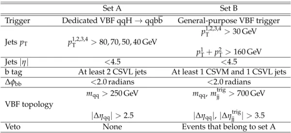
The offline event selection is based upon the b-jet and VBF-tagging jet assignment described in Section 5, and is adjusted to the two different trigger sets presented in Section 4. In what follows the selected events are divided into two sets referred to as set A and set B. These selections are summarized in Table 1.

Events selected in set A are required to have been selected by the dedicated VBF qqH→qqbb trigger and to have at least four PF jets with p1,2,3,4_T >80, 70, 50, 40 GeV and|η| <4.5. Moreover,

at least two of these jets must satisfy the loose CSV working point requirement (CSVL) [33]. The VBF topology is ensured by requiring mqq >250 GeV and|∆ηqq| > 2.5, where qq denotes

the pair of the most probable VBF-tagging jets. Finally, in order to suppress further the back-ground, the azimuthal angle difference∆φbbbetween the two b-jet candidates must be less than

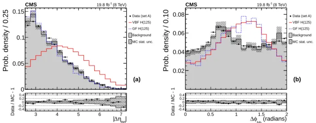
2.0 radians. Figure 1 shows the normalized distributions of|∆ηqq|(left) and∆φbb(right) for the

sum of all simulated backgrounds, and the VBF and GF Higgs boson production.

Events in set B are first required to not belong to set A (to avoid double counting). Then, they must have passed the generic VBF topological trigger and have at least four PF jets with pT >30 GeV and|η| <4.5. In addition, the scalar pTsum of the two leading jets must be greater

than 160 GeV. In order to enrich the sample in b jets, there must be at least one jet satisfying the medium CSV working point requirement (CSVM) [33] and one jet satisfying the CSVL. The VBF topology is ensured by requiring mqq, mtrigjj > 700 GeV, and|∆ηqq|, |∆ηjjtrig| > 3.5, where

qq denotes the pair of the most probable VBF jets and jj denotes the jet pair with the highest invariant mass (as in the trigger logic described in Section 4). Finally the azimuthal angle∆φbb

between the two b-jet candidates must be less than 2.0 radians.

After all the selection requirements, 2.3% of the simulated VBF signal events (for mH=125 GeV)

end up in set A, and 0.8% end up in set B. The fraction of events in set A that also satisfy the requirements of set B (except for the set A veto) amounts to 39%. The set B selection recovers signal events presenting pronounced VBF jets, with lower pT but larger pseudorapidity

open-ing and invariant mass.

Table 1: Summary of selection requirements for the two analyses.

Set A Set B

Trigger Dedicated VBF qqH→qqbb General-purpose VBF trigger p1,2,3,4_T >30 GeV Jets pT p1,2,3,4_T >80, 70, 50, 40 GeV

p1

T+p2T >160 GeV

Jets|η| <4.5 <4.5

b tag At least 2 CSVL jets At least 1 CSVM and 1 CSVL jets

∆φbb <2.0 radians <2.0 radians

mqq>250 GeV mqq, mtrig_jj >700 GeV

VBF topology

|∆η_qq| >2.5 |∆η_qq|,|∆η_jjtrig| >3.5

6 7 Signal properties Prob. density / 0.25 0 0.05 0.1 0.15 Data (set A) VBF H(125) GF H(125) Background MC stat. unc. (a) | qq η ∆ | 3 4 5 6 7 Data / MC - 1 -0.4 -0.20 0.2 0.4 (8 TeV) -1 19.8 fb CMS Prob. density / 0.10 0.02 0.04 0.06 0.08 Data (set A) VBF H(125) GF H(125) Background MC stat. unc. (b) (radians) bb φ ∆ 0 0.5 1 1.5 2 Data / MC - 1 -0.4 -0.20 0.2 0.4 (8 TeV) -1 19.8 fb CMS

Figure 1: (a) Normalized distribution in absolute pseudorapidity difference between the two VBF-jet candidates(|∆η_qq|). (b) Normalized distribution of the azimuthal difference between the two b-jet candidates (∆φ_bb). The selection corresponds to set A, data are shown by the points, and the sum of all simulated backgrounds is by the filled histograms. The VBF Higgs boson signal is displayed by a solid line, and the GF Higgs boson signal is shown by a dashed line. The panels at the bottom show the fractional difference between data and background simulation, with the shaded band representing the statistical uncertainties in the MC samples.

7

Signal properties

The analysis described in this paper relies on certain characteristic properties of the studied final state, which provide a significant improvement of the overall sensitivity. First, the reso-lution of the invariant mass of the two b jets is improved by applying multivariate regression techniques. Then, the jet composition properties are used to form a discriminant that separates jets originating from light quarks or gluons. Third, soft QCD activity outside the jets is quan-tified and used as a discriminant between QCD processes with strong color flow and the VBF signal without color flow.

7.1 Jet transverse-momentum regression

The bb mass resolution is improved by using a regression technique similar to those used in the search for a Higgs boson produced in association with a weak vector boson and decaying to bb [14]. A refined calibration is carried out for individual b jets, beyond the default jet energy corrections, that takes into account the jet composition properties and targets semileptonic b decays that lead to a substantial mismeasurement of the jet pT due to the presence of an

es-caping neutrino. For this purpose a regression BDT is trained on simulated signal events with inputs including information about the jet properties and structure. The target of the regres-sion is the pTof the associated particle-level jet, clustered from all stable particles (with lifetime

cτ > 1 cm). The inputs include: (i) the jet pT, η, and mass; (ii) the jet energy fractions carried

by neutral hadrons and photons [34–36]; (iii) the mass and the uncertainty in the decay length associated with the secondary vertex, when present; (iv) the event missing transverse energy and its azimuthal direction relative to the jet; (v) the total number of jet constituents; (vi) the pT

of the soft-lepton candidate inside the jet, when present, and its pTcomponent perpendicular

to the jet axis; (vii) the pTof the leading track in the jet; and (viii) the average pTdensity of the

event in y–φ space (FASTJETρmethod [42]).

The additional energy correction of b jets leads to an improvement of the jet pT resolution,

7.2 Discrimination between quark- and gluon-originated jets 7

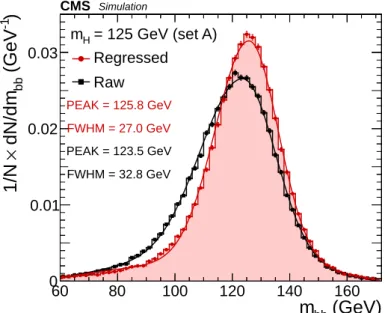
space of the offline event selections. Figure 2 shows the reconstructed dijet invariant mass of the b-jet candidates (mbb) before and after the regression for simulated events passing set A

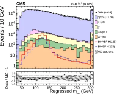
selections. The measured distribution of the regressed m_bbin set A is shown in Fig. 3.

The validation of the regression technique in data is done with samples of Z → `` events with one or two b-tagged jets. When the jets are corrected by the regression procedure, the pT

balance distribution, between the Z boson, reconstructed from the leptons, and the b-tagged jet or dijet system is improved to be better centered at zero and narrower than when the regression correction is not applied. In both cases the distributions for data and the simulated samples are in good agreement after the regression correction is applied.

(GeV)

m

)

(GeV

dN/dm

×

1/N

Figure 2: Simulated invariant mass distribution of the two b-jet candidates before and after the jet pTregression, for VBF signal events. The generated Higgs boson signal mass is 125 GeV and

the event selection corresponds to set A. By FWHM we denote the width of the distribution at the middle of its maximum height.

7.2 Discrimination between quark- and gluon-originated jets

To further identify whether the jet pair with the smallest b-tag values among the four leading jets is likely to originate from hadronization of a light (u,d,s-type) quark, as expected for signal VBF jets, or from gluons, as is more probable for jets produced in QCD processes, a quark-gluon discriminant [43–45] is applied to the VBF candidate jets.

The discriminant exploits differences in the showering and fragmentation of gluons and quarks, making use of the following internal jet composition observables based on the PF jet con-stituents: (i) the major root-mean square (RMS) of the distribution of jet constituents in the

η-φ plane [45], (ii) the minor RMS of the distribution of jet constituents in the η-φ plane [45],

(iii) the jet asymmetry pull [46], (iv) the jet particle multiplicity, and (v) the maximum energy fraction carried by a jet constituent. The pull and RMS variables are calculated by weighting each jet constituent by its pTsquared [45].

The five variables above are used as inputs to a likelihood estimated with gluon and quark jets from simulated QCD dijet events using the TMVA package. To improve the separation power, all variables are corrected for pileup effects as a function of the FASTJET ρ density. Figure 4

VBF-8 7 Signal properties

Events / 10 GeV

Figure 3: Distribution in invariant mass of the two b-jet candidates, after the jet pT regression,

for the events of set A. Data are shown by the points, while the simulated backgrounds are stacked. The LO QCD cross section is multiplied by a factor 1.68 so that the total number of background events equals the number of events in the data, while the VBF and GF Higgs boson signal cross sections are multiplied by a factor 10 for better visibility. The last bin is the sum of all the events beyond the range of the x axis (overflow). The panel at the bottom shows the fractional difference between the data and the background simulation, with the shaded band representing the statistical uncertainties in the MC samples.

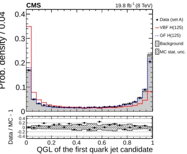
jet candidate (the jet that is ranked third in the b-tag score; see Section 5), for background and signal events. As expected, VBF signal events, dominated by quark jets, have a pronounced peak at likelihood ∼0, while the background and GF events are enriched in gluon jets, and have a very different QGL distribution. The QGL distribution of all four jets is used as input to the signal vs background discriminant (Section 9.1).

7.3 Soft QCD activity

To measure the additional hadronic activity between the VBF-tagging jets, excluding the more centrally produced Higgs boson decay products, only reconstructed charged tracks are used. This is done to measure the hadronic activity associated with the primary vertex (PV), defined as the reconstructed vertex with the largest sum of squared transverse momenta of tracks used to reconstruct it.

A collection of “additional tracks” is assembled using reconstructed tracks that (i) satisfy the high purity quality requirements defined in Ref. [47] and pT > 300 MeV; (ii) are not associated

with any of the four leading PF jets in the event; (iii) have a minimum longitudinal impact pa-rameter,|dz(PV)|, with respect to the main PV, rather than to other pileup interaction vertices;

(iv) satisfy |dz(PV)| < 2 mm and |dz(PV)| < 3σz(PV) with respect to the PV, where σz(PV)

is the uncertainty in dz(PV); and (v) are not in the region between the two best b-tagged jets.

This is defined as an ellipse in the η-φ plane, centered on the midpoint between the two jets, with major axis of length∆R(bb) +1, where ∆R(bb) = p(∆η_bb)2_{+ (}∆φ

bb)2, oriented along

the direction connecting the two b jets, and with minor axis of length 1.

The additional tracks are then clustered into “soft TrackJets” using the anti-kT clustering

9

Prob. density / 0.04

QGL of the first quark jet candidate

0 0.2 0.4 0.6 0.8 1 Data / MC - 1 -0.4 -0.2 0 0.2 0.4 (8 TeV) -1 19.8 fb CMS

Figure 4: Normalized distribution in quark-gluon likelihood discriminant of the first light-jet candidate. Quark jets are expected to have low likelihood values (closer to 0), while gluon jets are expected to have higher ones (closer to 1). The selection corresponds to set A, data are shown by the points, and the sum of all simulated backgrounds is shown by the filled his-togram. The VBF Higgs boson signal is displayed by a solid line, and the GF Higgs boson signal is shown by a dashed line. The panel at the bottom shows the fractional difference between the data and the background simulation, with the shaded band representing the statistical uncer-tainties in the MC samples.

method [48] to reconstruct the hadronization of partons with very low energies down to a few GeV [49]; an extensive study of the soft TrackJet activity can be found in Refs. [43, 44].

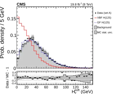
The discriminating variable, H_Tsoft, that encapsulates the differences between the signal and the QCD background, is the scalar pT sum of the soft TrackJets with pT > 1 GeV, and is shown in

Fig. 5.

8

Extraction of the Z boson signal

The Z +jets background process, with the Z boson decaying to a b-quark pair, provides a vali-dation of the analysis strategy used for the Higgs boson search. The extraction of the Z boson signal demonstrates the ability to observe a relatively wide hadronic resonance on top of a smooth QCD background. Also, if such a signal can be seen, it can serve for in situ confirma-tion of the scale and resoluconfirma-tion of the invariant mass of the two b jets. Recently, the observaconfirma-tion of a Z → bb signal was reported by the ATLAS Collaboration [50] in the Z +1 jet final state, and similar techniques are applied here. The overall strategy has two parts. First, events are selected from set A, with the additional requirement to have at least one CSVM jet. It should be noted that it is important to extract the Z boson signal in the same four-jet phase space in which the Higgs boson search is performed. Then, a multivariate discriminant is trained to separate the Z +jets process from the QCD multijet production, using variables that are only weakly correlated to mbb. According to the value of the discriminant the events are divided

into three categories, ranging from a signal-depleted control category, to a signal-enriched one. Finally, a simultaneous fit of the signal and the QCD background m_bbshape is performed in all three categories. The subsequent sections give details of the outlined procedure.

10 8 Extraction of the Z boson signal

Prob. density / 5 GeV

0 0.05 0.1 0.15 Data (set A) VBF H(125) GF H(125) Background MC stat. unc. (GeV) soft T H 0 20 40 60 80 100 120 140 Data / MC - 1 -0.4 -0.2 0 0.2 0.4 (8 TeV) -1 19.8 fb CMS

Figure 5: Normalized distribution of the scalar pTsum of TrackJets that are associated with the

soft QCD activity(Hsoft

T ). The selection corresponds to set A, data are shown by the points, and

the sum of all simulated backgrounds is shown by the filled histogram. The VBF Higgs boson signal is displayed by a solid line, and the GF Higgs boson signal is shown by a dashed line. The panel at the bottom shows the fractional difference between the data and the background simulation, with the shaded band representing the statistical uncertainties in the MC samples.

8.1 Z boson signal vs. background discrimination

As discussed above, the selection of events is based on set A, with the additional requirement of having at least one CSVM jet; the tightening of the b-tagging condition was found to im-prove the expected sensitivity. A Fisher discriminant (FD) [41] is implemented with the TMVA package and trained to discriminate between the Z +jets signal and the background. For this purpose, seven variables are used: (i) the absolute η difference|_∆ηqq|of the VBF jets; (ii) the ab-solute η of the b-jet system|η_bb|; (iii) the CSV value of the jet with highest CSV value (with best

b tag); and (iv)-(vii) the QGL values of the four leading jets. Due to the very small correlations between the variables, the FD performs almost as well as more advanced, nonlinear discrim-inators. Figure 6 shows the normalized distribution of the discriminant, where the output of the Z +jets signal is compared to the background.

8.2 Fit of the dijet invariant mass spectrum

The selected events are divided into three categories, based on the FD output. Table 2 summa-rizes the event categories and corresponding yields.

Table 2: Definition of the event categories for the Z boson signal extraction and corresponding yields in the mbbinterval[60, 170]GeV.

Category 1 Category 2 Category 3 FD< −0.02 −0.02<FD<0.02 FD>0.02

Data 659873 374797 342931

Z +jets 1374 1467 2783

tt 2124 1821 2327

8.2 Fit of the dijet invariant mass spectrum 11

Prob. density / 0.02

Z boson Fisher discriminant

-0.15 -0.1 -0.05 0 0.05 0.1 0.15 Data / MC - 1 -0.4 -0.2 0 0.2 0.4 (8 TeV) -1 19.8 fb CMS

Figure 6: Normalized distribution in Z boson Fisher discriminant. Data are shown by the points, and the sum of all simulated backgrounds is shown by the filled histogram. The Z +jets signal is displayed with solid line. The panel at the bottom shows the fractional differ-ence between the data and the background simulation, with the shaded band representing the statistical uncertainties in the MC samples.

Besides its discrimination power, the FD has minimal correlation with the invariant mass of the two b jets. This means that the mbb spectrum from QCD processes is independent of the

category. In practice, however, there is a small residual dependence, of up to 3%, which is corrected with a linear transfer function of mbb that is taken from data. The extraction of the

Z boson signal is done with a simultaneous fit in all three categories. Eq. (1) describes the fit model:

fi(mbb) =µZNi,ZZi(mbb; kJES, kJER) +Ni,tTi(mbb) +Ni,QCDKi(mbb)B8(mbb;~p), (1)

where the subscript i denotes the category, Ni,Zis the expected yield for the Z boson signal; and µZ, Ni,QCDare free parameters for the signal strength and the QCD event yield. The shape of the

top quark background Ti(mbb)is taken from the simulation (sum of the tt and single top quark

contributions), and the expected yield Ni,t is allowed to vary in the fit by 20%. The Z +jets

signal shape Zi(mbb; kJES, kJER)is taken from the simulation and is parametrized as a Crystal

Ball function [51] (Gaussian core with power-law tail) on top of a combinatorial background modeled by a polynomial. The position and the width of the Gaussian core are allowed to vary by the factors kJESand kJER, respectively, which quantify any mismatch of the jet energy scale

and resolution between data and simulation and are constrained by the dedicated validation measurements of the regressed jet energy scale and resolution.

Finally, the QCD background shape in each category is described by a common, eighth-order polynomial B8(mbb;~p), whose parameters ~p are determined by the fit, and a multiplicative

linear transfer function Ki(mbb)that accounts for the small background shape differences

be-tween the categories. The choice of the polynomial is based on an extensive bias study de-scribed in Section 9. Allowing for 20% uncertainty on the Z boson signal efficiency, the si-multaneous binned maximum-likelihood fit yields a signal strength of µZ = 1.10+−0.440.33, which

corresponds to an observed (expected) significance of 3.6 σ (3.3 σ). The fitted values of kJESand

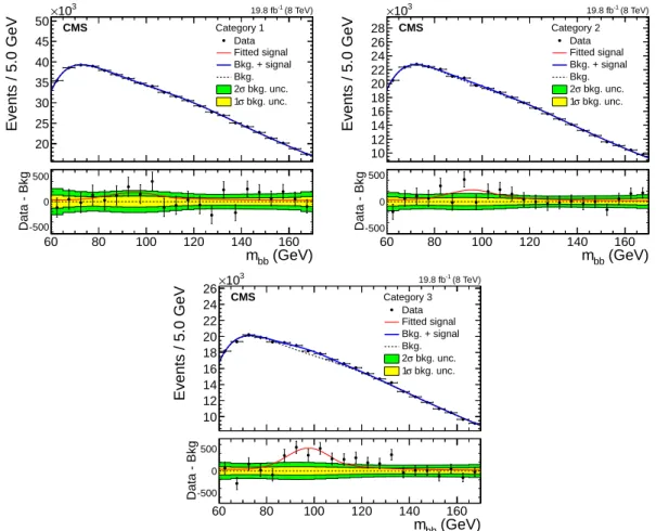
kJERare 1.01±0.02 and 1.02±0.10, respectively. Figure 7 shows the fitted distributions and the

12 9 Search for a Higgs boson

The extraction of the Z boson signal in this way validates the Higgs boson search method used in this paper by finding a known dijet resonance in a similar mass range. In addition, the simulated m_bbscale and resolution are consistent with the data, based on the best-fit values of the kJESand kJERnuisance parameters, which serve to constrain the corresponding uncertainties

in the Higgs boson signal extraction.

Events / 5.0 GeV 20 25 30 35 40 45 50 3 10 × (GeV) bb m 60 80 100 120 140 160 Data - Bkg-500 0 500 Category 1 Data Fitted signal Bkg. + signal Bkg. bkg. unc. σ 2 bkg. unc. σ 1 (8 TeV) -1 19.8 fb CMS Events / 5.0 GeV 10 12 14 16 18 20 22 24 26 28 3 10 × (GeV) bb m 60 80 100 120 140 160 Data - Bkg-500 0 500 Category 2 Data Fitted signal Bkg. + signal Bkg. bkg. unc. σ 2 bkg. unc. σ 1 (8 TeV) -1 19.8 fb CMS Events / 5.0 GeV 10 12 14 16 18 20 22 24 26 3 10 × (GeV) bb m 60 80 100 120 140 160 Data - Bkg-500 0 500 Category 3 Data Fitted signal Bkg. + signal Bkg. bkg. unc. σ 2 bkg. unc. σ 1 (8 TeV) -1 19.8 fb CMS

Figure 7: Invariant mass distribution of the two b-jet candidates for the Z boson signal in the three event categories that are based on the Z boson Fisher discriminant output, start-ing from the most backgroundlike (upper left) and endstart-ing at the most signal-like (bottom). Data are shown by the points. The solid line is the sum of the postfit background and signal shapes, while the dashed line is the background component alone. The bottom panel shows the background-subtracted distribution, overlaid with the fitted signal, and with the 1σ and 2σ background uncertainty bands. The measured (simulated) parameters of the Gaussian core of the signal shape in category 3 are 97.7 (96.6) GeV and 9.3 (9.1) GeV for the mean and the sigma, respectively.

9

Search for a Higgs boson

The search for a Higgs boson follows closely the methodology applied for the extraction of the Z boson signal (Section 8.2). Namely, a multivariate discriminant is employed (Section 9.1) to divide the events into seven categories that are subsequently fit simultaneously with mbb

9.1 Higgs boson signal vs. background discrimination 13

9.1 Higgs boson signal vs. background discrimination

In order to separate the overwhelmingly large QCD background from the Higgs boson signal, all discriminating features have to be used in an optimal way. This is best achieved by using a multivariate discriminant, which in this case is a BDT implemented with the TMVA package. The variables used as an input to the BDT are chosen such that they are very weakly correlated with the dynamics of the bb system, in particular with mbb, and are grouped into five distinct

groups: (i) the dynamics of the VBF-jet system, expressed by∆ηqq,∆φqq, and mqq; (ii) the b-jet

content of the event, expressed by the CSV output for the two best b-tagged jets; (iii) the jet flavor of the event QGL for all four jets; (iv) the soft activity, quantified by the scalar pT sum

H_Tsoft of the additional soft TrackJets with pT > 1 GeV, and the number Nsoft of soft TrackJets

with pT > 2 GeV; and (v) the angular dynamics of the production mechanism, expressed by

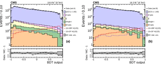
the cosine of the angle between the qq and bb planes in the center-of-mass frame of the four leading jets cos θ_qq,bb∗ . In practice, two BDTs are trained with the same input variables using the selections corresponding to the two sets of events. This distinction is necessary because the properties of the selected events are significantly different between the two selections (set A and set B). Figure 8 shows the output of the BDT for the two sets of events.

Events / 0.10 1 10 2 10 3 10 4 10 5 10 Data (set A)QCD (× 1.65) Z+jets t t Single t W+jets VBF H(125) × 10 GF H(125) × 10 MC stat. unc. (a) BDT output -1 -0.5 0 0.5 1 Data / MC - 1 -0.4 -0.2 0 0.2 0.4 (8 TeV) -1 19.8 fb CMS Events / 0.10 1 10 2 10 3 10 4 10 5 10 Data (set B) 1.80) × QCD ( Z+jets t t Single t W+jets VBF H(125) × 10 GF H(125) × 10 MC stat. unc. (b) BDT output -1 -0.5 0 0.5 1 Data / MC - 1 -0.4 -0.2 0 0.2 0.4 (8 TeV) -1 18.3 fb CMS

Figure 8: Distribution of the BDT output for the events of set A (a) and set B (b). Data are shown by the points, while the simulated backgrounds are stacked. The LO QCD cross sections are scaled such that the total number of background events equals the number of events in data, while the VBF and GF Higgs boson signal yields are multiplied by a factor of 10 for better visibility. The panels at the bottom show the fractional difference between the data and the background simulation, with the shaded band representing the statistical uncertainties of the MC samples.

9.2 Fit of the dijet invariant mass spectrum

Taking into account the expected sensitivity of the analysis and the available number of MC events (necessary to build the various mbb templates), seven categories are defined, according

to the BDT output: four for set A and three for set B. The boundaries of the categories and the respective event yields are summarized in Table 3. In an mbb interval of twice the width

of the Gaussian core of the signal distribution (mH = 125 GeV), the signal-over-background

ratio reaches 1.7% in the most sensitive category (category 4). It should be noted that both the VBF and GF contributions are added to the Higgs boson signal, with the fraction of the latter ranging from∼50% in category 1 to∼7% in category 4.

14 9 Search for a Higgs boson

Table 3: Definition of the event categories and corresponding yields in the mbb interval

[80, 200]GeV, for the data and the MC expectation. The BDT output boundary values refer to the distributions shown in Fig. 8.

BDT boundary values

set A set B

Cat. 1 Cat. 2 Cat. 3 Cat. 4 Cat. 5 Cat. 6 Cat. 7 −0.6 – 0.0 0.0 – 0.7 0.7 – 0.84 0.84 – 1.0 −0.1 – 0.4 0.4 – 0.8 0.8 – 1.0 Data 546121 321039 32740 10874 203865 108279 15151 Z +jets 2038 1584 198 71 435 280 45 W+jets 282 135 4 <1 225 92 17 tt 2818 839 45 14 342 169 21 Single t 960 633 64 25 194 159 30 VBF mH(125) 53 140 58 57 33 57 31 GF mH(125) 53 51 8 5 9 10 2

BDT categories of the same set of events. In reality, a small correction is needed to account for residual differences between the mbb spectrum in category 1 vs. categories 2,3 and 4, and in

category 5 vs. categories 6 and 7. The correction factor (transfer function) is a linear function of mbb in set A and a quadratic one in set B (because a stronger dependence is observed in

set B between mbb and the multivariate discriminant). With the introduction of the transfer

functions, the fit model for the Higgs boson signal is given by Eq. (2):

fi(mbb) =µHNi,HHi(mbb; kJES, kJER) +Ni,ZZi(mbb; kJES, kJER)

+Ni,tTi(mbb; kJES, kJER) +Ni,QCDKi(mbb)B(mbb;~pset),

(2) where the subscript i denotes the category and µH, Ni,QCD are free parameters for the signal

strength and the QCD event yield. Ni,H, Ni,Z, and Ni,t are the expected yields for the Higgs

boson signal, the Z +jets, and the top quark background respectively. The shape of the top quark background Ti(mbb; kJES, kJER) is taken from the simulation (sum of the tt and single

top quark contributions) and is described by a broad Gaussian. The Z/W+jets background Zi(mbb; kJES, kJER)and the Higgs boson signal Hi(mbb; kJES, kJER)shapes are taken from the

sim-ulation and are parametrized as a Crystal Ball function (Gaussian core with power-law tail) on top of a polynomial. The position and the width of the Gaussian core of the MC templates (sig-nal and background) are allowed to vary by the free factors kJESand kJER, respectively, which

quantify any mismatch of the jet energy scale and resolution between data and simulation. Finally, the QCD shape is described by a polynomial B(mbb;~pset), common within the

cate-gories of each set, and a multiplicative transfer function Ki(mbb)per category, accounting for

the shape differences between the categories. The parameters of the polynomial,~pset, and those

of the transfer functions, are determined by the fit, which is performed simultaneously in all categories in each set. For set A, the polynomial is of fifth order, while for set B it is of fourth order.

The choice of the QCD background shapes and event category transfer function parametriza-tions are fully based on data, and have been performed among classes of funcparametriza-tions, e.g. poly-nomials, exponential, power laws and their combinations, with a minimum number of degrees of freedom suited to fit the data in all categories. Each function considered is used to generate different MC pseudo-data sets, and each data set is fitted using the different functional models. A potential bias on the signal estimation is computed for each pair of possible functions used to generate and fit to the pseudo-data sets. The background model chosen yields a maximum potential bias on the fitted signal strength of less than six times the statistical uncertainty on the background. Hence the systematic uncertainty associated with the background shape can be neglected.

15

10

Systematic uncertainties

Table 4 summarizes the sources of uncertainty related to both the background and to the signal processes. The leading uncertainty comes from the QCD background description: both the pa-rameters of its shape and the overall normalization in each category are allowed to float freely, being determined by the simultaneous fit to the data. The resulting covariance matrix is used to compute the uncertainty. For the smaller background contributions from the Z/W+jets and top quark production, the mbb shapes are taken from the simulation, while their

correspond-ing yields are allowed to float in the fit with a 30% log-normal constraint centered on the SM expectations.

The experimental uncertainties on the jet energy scale (JES) and jet energy resolution (JER) affect the signal acceptance and the shape of the multivariate discriminant output, and are in-cluded as nuisance parameters. The effect of the JES and JER uncertainties on the mbb shape

is taken into account in the fit function. By varying the JES and JER by their measured uncer-tainties [39], the impact of the signal yield per analysis category is estimated. These variations affect the acceptance by up to 10%, while the peak position of the mbb shape is shifted by 2%,

and the width by 10%.

Additional uncertainties are assigned to the flavor tagging of the jets. The CSV and QGL dis-criminant outputs are shifted according to the observed agreement between data and simu-lation and the effect on the signal acceptance is estimated to range from 3% to 10% for the former, and from 1% to 3% for the latter. The impact of the CSV shift is more significant, both because it is used for the event selection, and because the multivariate discriminant depends more strongly on the b tagging of the jets. The shift of QGL only affects the shape of the dis-criminant, and thus the distribution of signal events in the analysis categories.

The trigger uncertainty is estimated by propagating the uncertainty in the data vs. MC simu-lation scale factor for the efficiency. This is achieved by convolving the two-dimensional effi-ciency scale factor with the signal distribution. As a result, the uncertainty in the signal yield ranges from 1% to 6% for the VBF process, and from 5% to 20% for the GF.

Theoretical uncertainties affect the signal simulation. First, the uncertainty due to PDFs and strong coupling constant αSvariation is computed to be 2.8% (VBF) and 7.5% (GF) [52]. A

resid-ual uncertainty from these sources is estimated for the particular kinematical phase space of the search: following the PDF4LHC prescription [53, 54] the PDF and αSuncertainty ranges from

2% to 5%, while the renormalization and factorization scale variations in the signal simulation induce an uncertainty of 1% to 5% in the analysis categories, on top of a global cross section un-certainty of 0.2% (VBF) and 7.7–8.1% (GF). Finally, the variation of the UE and parton-shower (PS) model (usingPYTHIA8.1 [55] instead of the defaultPYTHIA6) affects the signal acceptance by 2% to 7% (VBF) and by 10% to 45% (GF).

Lastly, an uncertainty of 2.6% is assigned to the total integrated luminosity measurement [56].

11

Results

The mbb distributions in data, for all categories, are fitted simultaneously with the

paramet-ric functions described in Section 9.2 under two different hypotheses: background only and background plus a Higgs boson signal. The fit is a binned likelihood fit incorporating the sys-tematic uncertainties discussed in Section 10 as nuisance parameters. Due to the smallness of the GF contribution in the most signal-sensitive categories we do not attempt to fit inde-pendently the VBF and the GF signal strengths. The fits in sets A and B are shown in Figs. 9 and 10, respectively. The limits on the signal strength are computed with the asymptotic CLs

16 12 Combination with other CMS Higgs boson to b-quarks searches

Table 4: Sources of systematic uncertainty and their impact on the shape and normalization of the background and signal processes.

Background uncertainties

QCD shape parameters determined by the fit QCD bkg. normalization determined by the fit Top quark bkg. normalization 30%

Z/W+jets bkg. normalization 30%

Uncertainties affecting the signal VBF signal GF signal

JES (signal shape) 2%

JER (signal shape) 10%

Integrated luminosity 2.6% Branching fraction (H→bb) 2.4%–4.3% JES (acceptance) 6%–10% 4%–12% JER (acceptance) 1%–4% 1%–9% b-jet tagging 3%–9% 3%–10% Quark/gluon-jet tagging 1%–3% 1%–3% Trigger 1%–6% 5%–20%

Theory uncertainties VBF signal GF signal

UE & PS 2%–7% 10%–45%

Scale variation (global) 0.2% 7.7%–8.1% Scale variation (categories) 1%–5% 1%–5%

PDF (global) 2.8% 7.5%

PDF (categories) 1.5%–3% 3.5%–5%

method [57–59]. Figure 11 shows the observed (expected) 95% confidence level (CL) limit on the total VBF plus GF signal strength, as a function of the Higgs boson mass, which ranges from 5.0 (2.2) at mH =115 GeV to 5.8 (3.7) at mH =135 GeV, together with the expected limits in the

presence of a SM Higgs boson with a mass of 125 GeV. For the 125 GeV Higgs boson signal the observed (expected) significance is 2.2 (0.8) standard deviations, and the fitted signal strength is µ= σ/σSM =2.8+−1.61.4. The measured signal strength is compatible with the SM Higgs boson

prediction µ=1 at the 8% level.

12

Combination with other CMS Higgs boson to b-quarks searches

The CMS experiment has also performed searches for the Higgs boson decaying to bottom quarks, where the Higgs boson is produced in association with a vector boson [14] (VH), or with a top quark pair [16, 17] (ttH). The VH results have been recently updated and combined with ttH [11]. Here we combine those results with the ones from the VBF production search described in this paper. Event selection overlaps between different analyses have been checked and are either empty by construction or have negligible effects on the combination. The com-bination methodology is based on the likelihood ratio test statistics employed in Section 11, and takes into account correlations among sources of systematic uncertainty. Care is taken to understand the behavior of the parameters that are correlated between analyses, in terms of the fitted parameter values and uncertainties.

Table 5 lists the 95% CL expected and observed upper limits and the best-fit signal strength values from the individual channels and from the combined fit. For mH = 125 GeV the

com-bination yields an H → bb signal strength µ = 1.03+₋0.44_0.42 with a significance of 2.6 standard deviations.

17 Events / 2.5 GeV 6000 8000 10000 12000 14000 16000 18000 20000 22000 (GeV) bb m 80 100 120 140 160 180 200 Data - Bkg -400 -200 0 200 400 Category 1 Data Fitted signal (m = 125 GeV)H Bkg. + signal Bkg. QCD bkg. unc. σ 2 bkg. unc. σ 1 CMS (8TeV) -1 19.8 fb Events / 2.5 GeV 4000 6000 8000 10000 12000 (GeV) bb m 80 100 120 140 160 180 200 Data - Bkg -300 -200 -100 0 100 200 300 Category 2 Data Fitted signal (m = 125 GeV)H Bkg. + signal Bkg. QCD bkg. unc. σ 2 bkg. unc. σ 1 CMS (8TeV) -1 19.8 fb Events / 2.5 GeV 400 600 800 1000 1200 (GeV) bb m 80 100 120 140 160 180 200 Data - Bkg -100 -50 0 50 100 Category 3 Data Fitted signal (m = 125 GeV)H Bkg. + signal Bkg. QCD bkg. unc. σ 2 bkg. unc. σ 1 CMS (8TeV) -1 19.8 fb Events / 2.5 GeV 100 150 200 250 300 350 400 450 (GeV) bb m 80 100 120 140 160 180 200 Data - Bkg -50 0 50 Category 4 Data Fitted signal (m = 125 GeV)H Bkg. + signal Bkg. QCD bkg. unc. σ 2 bkg. unc. σ 1 CMS (8TeV) -1 19.8 fb

Figure 9: Fit of the invariant mass of the two b-jet candidates for the Higgs boson signal (mH =

125 GeV) in the four event categories of set A. Data are shown by the points. The solid line is the sum of the postfit background and signal shapes, the dashed line is the background component, and the dashed-dotted line is the QCD component alone. The bottom panel shows the background-subtracted distribution, overlaid with the fitted signal, and with the 1σ and 2σ background uncertainty bands.

18 13 Summary Events / 2.5 GeV 2000 3000 4000 5000 6000 7000 8000 9000 (GeV) bb m 80 100 120 140 160 180 200 Data - Bkg -400 -200 0 200 400 Category 5 Data Fitted signal (m = 125 GeV) H Bkg. + signal Bkg. QCD bkg. unc. σ 2 bkg. unc. σ 1 CMS (8TeV) -1 18.3 fb Events / 2.5 GeV 1000 1500 2000 2500 3000 3500 4000 4500 5000 (GeV) bb m 80 100 120 140 160 180 200 Data - Bkg -200 -100 0 100 200 Category 6 Data Fitted signal (m = 125 GeV) H Bkg. + signal Bkg. QCD bkg. unc. σ 2 bkg. unc. σ 1 CMS (8TeV) -1 18.3 fb Events / 2.5 GeV 200 300 400 500 600 700 (GeV) bb m 80 100 120 140 160 180 200 Data - Bkg -50 0 50 Category 7 Data Fitted signal (m = 125 GeV)H Bkg. + signal Bkg. QCD bkg. unc. σ 2 bkg. unc. σ 1 CMS (8TeV) -1 18.3 fb

Figure 10: Fit of the invariant mass of the two b-jet candidates for the Higgs boson signal (mH= 125 GeV) in the three event categories of set B. Data are shown with markers. The solid

line is the sum of the postfit background and signal shapes, the dashed line is the background component, and the dashed-dotted line is the QCD component alone. The bottom panel shows the background-subtracted distribution, overlaid with the fitted signal, and with the 1σ and 2σ background uncertainty bands.

13

Summary

A search has been carried out for the SM Higgs boson produced in vector boson fusion and decaying to bb with two data samples of pp collisions at√s = 8 TeV collected with the CMS detector at the LHC corresponding to integrated luminosities of 19.8 fb−1and 18.3 fb−1. Upper limits, at the 95% confidence level, on the production cross section times the H→bb branching fraction, relative to expectations for a SM Higgs boson, are extracted for a Higgs boson in the mass range 115–135 GeV. In this range, the expected upper limits in the absence of a signal vary between a factor of 2.2 to 3.7 of the SM prediction, while the observed upper limits vary from 5.0 to 5.8. For a Higgs boson mass of 125 GeV, the observed and expected significance is, respectively, 2.2 and 0.8 standard deviations, and the fitted signal strength is µ = σ/σSM =

2.8+₋1.6_1.4. This is the first search of this kind, and the only search for the SM Higgs boson in all-jet final states, at the LHC.

The combination of the results obtained in this search with other CMS H→bb searches in the VH and ttH production modes, yields a H → bb signal strength µ = 1.03+₋0.44_0.42 with a signal significance of 2.6 standard deviations for mH =125 GeV that is consistent with the SM.

19

Higgs Boson Mass (GeV)

115 120 125 130 135 SM

σ

/

σ

9

5

%

A

s

y

m

p

to

ti

c

C

L

L

im

it

o

n

Exp. for SM m = 125 GeV_H

Expected (68%) Expected (95%) CMS (8TeV) -1 19.8 fb

Figure 11: Expected and observed 95% confidence level limits on the signal cross section in units of the SM expected cross section, as a function of the Higgs boson mass, including all event categories. The limits expected in the presence of a SM Higgs boson with a mass of 125 GeV are indicated by the dotted curve.

Table 5: Observed and expected 95% CL limits, best fit values on the signal strength parameter

µ = σ/σSM and signal significances for mH = 125 GeV, for each H → bb channel and their

combination.

H→bb Best fit (68% CL) Upper limits (95% CL) Signal significance Channel Observed Observed Expected Observed Expected

VH 0.89±0.43 1.68 0.85 2.08 2.52

ttH 0.7±1.8 4.1 3.5 0.37 0.58

VBF 2.8+₋1.6_1.4 5.5 2.5 2.20 0.83

20 References

Acknowledgments

We congratulate our colleagues in the CERN accelerator departments for the excellent perfor-mance of the LHC and thank the technical and administrative staffs at CERN and at other CMS institutes for their contributions to the success of the CMS effort. In addition, we gratefully acknowledge the computing centers and personnel of the Worldwide LHC Computing Grid for delivering so effectively the computing infrastructure essential to our analyses. Finally, we acknowledge the enduring support for the construction and operation of the LHC and the CMS detector provided by the following funding agencies: BMWFW and FWF (Austria); FNRS and FWO (Belgium); CNPq, CAPES, FAPERJ, and FAPESP (Brazil); MES (Bulgaria); CERN; CAS, MoST, and NSFC (China); COLCIENCIAS (Colombia); MSES and CSF (Croatia); RPF (Cyprus); MoER, ERC IUT and ERDF (Estonia); Academy of Finland, MEC, and HIP (Finland); CEA and CNRS/IN2P3 (France); BMBF, DFG, and HGF (Germany); GSRT (Greece); OTKA and NIH (Hungary); DAE and DST (India); IPM (Iran); SFI (Ireland); INFN (Italy); MSIP and NRF (Re-public of Korea); LAS (Lithuania); MOE and UM (Malaysia); CINVESTAV, CONACYT, SEP, and UASLP-FAI (Mexico); MBIE (New Zealand); PAEC (Pakistan); MSHE and NSC (Poland); FCT (Portugal); JINR (Dubna); MON, RosAtom, RAS and RFBR (Russia); MESTD (Serbia); SEIDI and CPAN (Spain); Swiss Funding Agencies (Switzerland); MST (Taipei); ThEPCenter, IPST, STAR and NSTDA (Thailand); TUBITAK and TAEK (Turkey); NASU and SFFR (Ukraine); STFC (United Kingdom); DOE and NSF (USA).

Individuals have received support from the Marie-Curie program and the European Research Council and EPLANET (European Union); the Leventis Foundation; the A. P. Sloan Founda-tion; the Alexander von Humboldt FoundaFounda-tion; the Belgian Federal Science Policy Office; the Fonds pour la Formation `a la Recherche dans l’Industrie et dans l’Agriculture (FRIA-Belgium); the Agentschap voor Innovatie door Wetenschap en Technologie (IWT-Belgium); the Ministry of Education, Youth and Sports (MEYS) of the Czech Republic; the Council of Science and In-dustrial Research, India; the HOMING PLUS program of the Foundation for Polish Science, co-financed from the European Union, Regional Development Fund; the Compagnia di San Paolo (Torino); the Consorzio per la Fisica (Trieste); MIUR project 20108T4XTM (Italy); the Thalis and Aristeia programs cofinanced by EU-ESF and the Greek NSRF; and the National Priorities Research Program by the Qatar National Research Fund.

References

[1] A. Salam, “Weak and electromagnetic interactions”, in Elementary particle physics: relativistic groups and analyticity, N. Svartholm, ed., p. 367. Almqvist & Wiksell, Stockholm, 1968. Proceedings of the eighth Nobel symposium.

[2] S. L. Glashow, “Partial-symmetries of weak interactions”, Nucl. Phys. 22 (1961) 579, doi:10.1016/0029-5582(61)90469-2.

[3] S. Weinberg, “A Model of Leptons”, Phys. Rev. Lett. 19 (1967) 1264, doi:10.1103/PhysRevLett.19.1264.

[4] F. Englert and R. Brout, “Broken Symmetry and the Mass of Gauge Vector Mesons”, Phys. Rev. Lett. 13 (1964) 321, doi:10.1103/PhysRevLett.13.321.

[5] P. W. Higgs, “Broken Symmetries and the Masses of Gauge Bosons”, Phys. Rev. Lett. 13 (1964) 508, doi:10.1103/PhysRevLett.13.508.

References 21

[6] G. S. Guralnik, C. R. Hagen, and T. W. B. Kibble, “Global Conservation Laws and Massless Particles”, Phys. Rev. Lett. 13 (1964) 585,

doi:10.1103/PhysRevLett.13.585.

[7] ATLAS Collaboration, “Observation of a new particle in the search for the Standard Model Higgs boson with the ATLAS detector at the LHC”, Phys. Lett. B 716 (2012) 1, doi:10.1016/j.physletb.2012.08.020, arXiv:1207.7214.

[8] CMS Collaboration, “Observation of a new boson at a mass of 125 GeV with the CMS experiment at the LHC”, Phys. Lett. B 716 (2012) 30,

doi:10.1016/j.physletb.2012.08.021, arXiv:1207.7235.

[9] CMS Collaboration, “Observation of a new boson with mass near 125 GeV in pp collisions at√s = 7 and 8 TeV”, JHEP 06 (2013) 081,

doi:10.1007/JHEP06(2013)081, arXiv:1303.4571.

[10] ATLAS Collaboration, “Measurements of Higgs boson production and couplings in diboson final states with the ATLAS detector at the LHC”, Phys. Lett. B 726 (2013) 88, doi:10.1016/j.physletb.2013.08.010, arXiv:1307.1427. [Erratum: doi::10.1016/j.physletb.2014.05.011].

[11] CMS Collaboration, “Precise determination of the mass of the Higgs boson and tests of compatibility of its couplings with the standard model predictions using proton

collisions at 7 and 8 TeV”, Eur. Phys. J. C 75 (2015) 212,

doi:10.1140/epjc/s10052-015-3351-7, arXiv:1412.8662.

[12] LHC Higgs Cross Section Working Group, S. Dittmaier et al., “Handbook of LHC Higgs Cross Sections: 2. Differential Distributions”, CERN Report CERN-2012-002, 2012. doi:10.5170/CERN-2012-002, arXiv:1201.3084.

[13] CDF and D0 Collaboration, “Evidence for a Particle Produced in Association with Weak Bosons and Decaying to a Bottom-Antibottom Quark Pair in Higgs Boson Searches at the Tevatron”, Phys. Rev. Lett. 109 (2012) 071804,

doi:10.1103/PhysRevLett.109.071804, arXiv:1207.6436.

[14] CMS Collaboration, “Search for the standard model Higgs boson produced in association with W or Z bosons and decaying to bottom quarks”, Phys. Rev. D 89 (2014) 012003, doi:10.1103/PhysRevD.89.012003, arXiv:1310.3687.

[15] ATLAS Collaboration, “Search for the bbar decay of the Standard Model Higgs boson in associated (W/Z)H production with the ATLAS detector”, JHEP 01 (2015) 069,

doi:10.1007/JHEP01(2015)069, arXiv:1409.6212.

[16] CMS Collaboration, “Search for the standard model Higgs boson produced in association with a top-quark pair in pp collisions at the LHC”, JHEP 05 (2013) 145,

doi:10.1007/JHEP05(2013)145, arXiv:1303.0763.

[17] CMS Collaboration, “Search for the associated production of the Higgs boson with a top-quark pair”, JHEP 09 (2014) 087, doi:10.1007/JHEP09(2014)087,

arXiv:1408.1682.

[18] ATLAS Collaboration, “Search for the Standard Model Higgs boson produced in

association with top quarks and decaying into b ¯b in pp collisions at√s = 8 TeV with the ATLAS detector”, (2015). arXiv:1503.05066. Submitted to EPJC.

22 References

[19] CDF Collaboration, “Search for the Higgs boson in the all-hadronic final state using the full CDF data set”, JHEP 02 (2013) 004, doi:10.1007/JHEP02(2013)004,

arXiv:1208.6445.

[20] CMS Collaboration, “The CMS experiment at the CERN LHC”, JINST 3 (2008) S08004, doi:10.1088/1748-0221/3/08/S08004.

[21] P. Nason, “A New method for combining NLO QCD with shower Monte Carlo algorithms”, JHEP 11 (2004) 040, doi:10.1088/1126-6708/2004/11/040, arXiv:hep-ph/0409146.

[22] P. Golonka et al., “The tauola-photos-F environment for the TAUOLA and PHOTOS packages, release II”, Comp. Phys. Commun. 174 (2006) 818,

doi:10.1016/j.cpc.2005.12.018, arXiv:hep-ph/0312240.

[23] T. Sj ¨ostrand, S. Mrenna, and P. Skands, “PYTHIA 6.4 physics and manual”, JHEP 05 (2006) 026, doi:10.1088/1126-6708/2006/05/026, arXiv:hep-ph/0603175. [24] R. Field, “Early LHC Underlying Event Data - Findings and Surprises”, (2010).

arXiv:1010.3558.

[25] J. Pumplin et al., “New Generation of Parton Distributions with Uncertainties from Global QCD Analysis”, JHEP 07 (2012) 012,

doi:10.1088/1126-6708/2002/07/012, arXiv:hep-ph/0201195. [26] J. Alwall et al., “MadGraph 5: going beyond”, JHEP 06 (2011) 128,

doi:10.1007/JHEP06(2011)128, arXiv:1106.0522.

[27] H.-L. Lai et al., “New parton distributions for collider physics”, Phys. Rev. D 82 (2010) 074024, doi:10.1103/PhysRevD.82.074024, arXiv:1007.2241.

[28] R. Gavin, Y. Li, F. Petriello, and S. Quackenbush, “FEWZ 2.0: A code for hadronic Z production at next-to-next-to-leading order”, Comput. Phys. Commun. 182 (2011) 2388, doi:10.1016/j.cpc.2011.06.008, arXiv:1011.3540.

[29] Y. Li and F. Petriello, “Combining QCD and electroweak corrections to dilepton production in the framework of the FEWZ simulation code”, Phys. Rev. D 86 (2012) 094034, doi:10.1103/PhysRevD.86.094034, arXiv:1208.5967.

[30] R. Gavin, Y. Li, F. Petriello, and S. Quackenbush, “W physics at the LHC with FEWZ 2.1”, Comput. Phys. Commun. 184 (2013) 208, doi:10.1016/j.cpc.2012.09.005,

arXiv:1201.5896.

[31] M. Czakon, P. Fiedler, and A. Mitov, “Total Top-Quark Pair-Production Cross Section at Hadron Colliders Through O(α4

S)”, Phys. Rev. Lett. 110 (2013) 252004,

doi:10.1103/PhysRevLett.110.252004, arXiv:1303.6254.

[32] N. Kidonakis, “Differential and total cross sections for top pair and single top production”, (2012). arXiv:1205.3453.

[33] CMS Collaboration, “Identification of b-quark jets with the CMS experiment”, JINST 8 (2013) P04013, doi:10.1088/1748-0221/8/04/P04013, arXiv:1211.4462.

[34] CMS Collaboration, “Particle–flow event reconstruction in CMS and performance for jets, taus, and Emiss_T ”, CMS Physics Analysis Summary CMS-PAS-PFT-09-001, CERN, 2009.

References 23

[35] CMS Collaboration, “Commissioning of the Particle-flow Event Reconstruction with the first LHC collisions recorded in the CMS detector”, CMS Physics Analysis Summary CMS-PAS-PFT-10-001, CERN, 2010.

[36] CMS Collaboration, “Commissioning of the particle-flow reconstruction in minimum-bias and jet events from pp collisions at 7 TeV”, CMS Physics Analysis Summary CMS-PAS-PFT-10-002, CERN, 2010.

[37] M. Cacciari and G. P. Salam, “Dispelling the N3myth for the ktjet-finder”, Phys. Lett. B

641(2006) 57, doi:10.1016/j.physletb.2006.08.037, arXiv:hep-ph/0512210. [38] M. Cacciari, G. P. Salam, and G. Soyez, “The anti-ktjet clustering algorithm”, JHEP 04

(2008) 063, doi:10.1088/1126-6708/2008/04/063, arXiv:0802.1189.

[39] CMS Collaboration, “Determination of jet energy calibration and transverse momentum resolution in CMS”, J. Instrum. 6 (2011) P11002,

doi:10.1088/1748-0221/6/11/P11002.

[40] CMS Collaboration, “Pileup jet identification”, CMS Physics Analysis Summary CMS-PAS-JME-13-005, CERN, 2013.

[41] H. Voss, A. H ¨ocker, J. Stelzer, and F. Tegenfeldt, “TMVA, the Toolkit for Multivariate Data Analysis with ROOT”, in XIth International Workshop on Advanced Computing and Analysis Techniques in Physics Research (ACAT), p. 40. 2007. arXiv:physics/0703039.

[42] M. Cacciari and G. P. Salam, “Pileup subtraction using jet areas”, Phys. Lett. B 659 (2008) 119, doi:10.1016/j.physletb.2007.09.077, arXiv:0707.1378.

[43] CMS Collaboration, “Measurement of the hadronic activity in events with a Z and two jets and extraction of the cross section for the electroweak production of a Z with two jets in pp collisions at√s = 7 TeV”, JHEP 10 (2013) 101,

doi:10.1007/JHEP10(2013)062, arXiv:1305.7389.

[44] CMS Collaboration, “Measurement of electroweak production of two jets in association with a Z boson in proton-proton collisions at√s=8 TeV”, Eur. Phys. J. C 75 (2015) 66, doi:10.1140/epjc/s10052-014-3232-5, arXiv:1410.3153.

[45] CMS Collaboration, “Performance of quark/gluon discrimination in 8 TeV pp data”, CMS Physics Analysis Summary CMS-PAS-JME-13-002, CERN, 2013.

[46] J. Gallicchio and M. D. Schwartz, “Seeing in Color: Jet Superstructure”, Phys. Rev. Lett.

105(2010) 022001, doi:10.1103/PhysRevLett.105.022001, arXiv:1001.5027. [47] CMS Collaboration, “CMS tracking performance results from early LHC operation”, Eur.

Phys. J. C 70 (2010) 1165, doi:10.1140/epjc/s10052-010-1491-3, arXiv:1007.1988.

[48] CMS Collaboration, “Commissioning of trackjets in pp collisions at√s=7 TeV”, CMS Physics Analysis Summary CMS-PAS-JME-10-006, CERN, 2010.

[49] CMS Collaboration, “Performance of jet reconstruction with charged tracks only”, CMS Physics Analysis Summary CMS-PAS-JME-08-001, CERN, 2009.

24 References

[50] ATLAS Collaboration, “Measurement of the cross section of high transverse momentum Z→b ¯b production in proton–proton collisions at√s = 8 TeV with the ATLAS Detector”, Phys. Lett. B 738 (2014) 25, doi:10.1016/j.physletb.2014.09.020,

arXiv:1404.7042.

[51] M. J. Oreglia, “A study of the reactions ψ0 →γγψ”. PhD thesis, Stanford University,

1980. SLAC Report SLAC-R-236, see Appendix D.

[52] S. Heinemeyer et al., “Handbook of LHC Higgs cross sections: 3. Higgs properties”, CERN Report CERN-2013-004, 2013. doi:10.5170/CERN-2013-004,

arXiv:1307.1347.

[53] S. Alekhin et al., “The PDF4LHC Working Group Interim Report”, (2011). arXiv:1101.0536.

[54] M. Botje et al., “The PDF4LHC Working Group Interim Recommendations”, (2011). arXiv:1101.0538.

[55] T. Sj ¨ostrand, S. Mrenna, and P. Skands, “A brief introduction to PYTHIA 8.1”, Comput. Phys. Commun. 178 (2008) 852, doi:10.1016/j.cpc.2008.01.036,

arXiv:0710.3820.

[56] CMS Collaboration, “CMS luminosity based on pixel cluster counting - summer 2013 update”, CMS Physics Analysis Summary CMS-PAS-LUM-13-001, CERN, 2013. [57] T. Junk, “Confidence level computation for combining searches with small statistics”,

Nucl. Instrum. Meth. A 434 (1999) 435, doi:10.1016/S0168-9002(99)00498-2. [58] A. L. Read, “Presentation of search results: the CLstechnique”, J. Phys. G 28 (2002) 2693,

doi:10.1088/0954-3899/28/10/313.

[59] G. Cowan, K. Cranmer, E. Gross, and O. Vitells, “Asymptotic formulae for likelihood-based tests of new physics”, Eur. Phys. J. C 71 (2011) 1554, doi:10.1140/epjc/s10052-011-1554-0, arXiv:1007.1727.