Dynamic QoS Management for Ethernet-based Video Surveillance Systems

F

E

U

P

Dynamic QoS Management for

Ethernet-based Video Surveillance

Systems

Tiago José da Silva Rocha

Mestrado Integrado em Engenharia Eletrotécnica e de Computadores Supervisor: Professor Doutor Luís Miguel Pinho de Almeida

Resumo

Os sistemas de videovigilância têm vindo a ser implementados em várias áreas ao longo dos anos, como por exemplo, segurança, controlo de acessos ou monitorização de processos industriais. À medida que os casos de uso aumentam, aumenta também a necessidade de que estes proporcionem a melhor qualidade de imagem, utilizando o mínimo de recursos possível, nomeadamente largura de banda, diminuindo assim os custos. Atualmente, as câmaras profissionais dispoem de fun-cionalidades de controlo de transmissão que oferecerem transmissão a taxas constantes (CBR) e majoradas (MBR), limitando a largura de banda utilizada. No entanto, estas carecem de eficiência na utlização da largura de banda, quando utilizadas em sistemas com várias câmaras, capturando diferentes cenários, que podem mudar de um momento para o outro. Este problema necessita de uma solução de gestão global, capaz de te ter uma visão geral das necessidades de todas as câmaras e tomar decisões de redistribuição da largura de banda consoante essas necessidades.

Esta dissertação descreve um sistema de videovigilância com gestão dinâmica de qualidade de serviço, que utiliza um gestor de rede para redistribuir a largura de banda global do sistema dinamicamente, de acordo com as necessidades de cada câmara; e implementa um controlador PI local de compressão de imagem, para que cada câmara possa adaptar-se à largura de banda que lhe é atribuída. A distribuição da largura de banda é baseada na teoria dos jogos, usa Linux TC para aplicar as reservas de largura de banda diretamente nas câmaras e adapta os valores de largura de banda atribuídos de forma a balancear as qualidades das imagens de todas as câmaras. Este balanceamento foi implementado através de um fator matemático, desenvolvido numa base empírica, que foi integrado no controlador do gestor de rede.

As experiências realizadas consistiram na alocação de um valor constante de largura de banda para provar a capacidade de adaptação utilizando o controlador local; a ligação ao sistema de duas câmaras em instantes diferentes, com imagens diferentes, para mostrar a eficácia da distribuição feita pelo gestor; e a ligação de até três câmaras para mostrar a escalabilidade do sistema e a eficácia do balanceamento de qualidades.

Os resultados foram satisfatórios no que diz respeito à distribuição da largura de banda e ao controlo de compressão. Relativamente ao balanceamento da qualidade de imagem entre as câ-maras, o mecanismo criado gerou resultados promissores. No entanto, não foi possível fazer, em tempo útil, um estudo aprofundado do mesmo de forma a otimizá-lo. Os objetivos propostos rel-ativamente à possibilidade de definir uma câmara "em foco", que teria uma qualidade de imagem superior às restantes não foi conseguido.

Abstract

Video surveillance systems have been implemented in several areas over the years, namely, se-curity, access control, monitoring of industrial processes, and, as the use cases increase, so does the need for them to provide the best quality using the minimum of resources, namely bandwidth, thus lowering its costs. Although the state-of-the-art rate control features implemented in profes-sional cameras offer Constant Bit Rate (CBR) and Maximum Bit Rate (MBR), which limit the bandwidth used, these still lack efficiency in bandwidth utilization when used in systems with several cameras, capturing different scenarios that may change from time to time. This calls for a dynamic global management solution, capable of having an overview of the camera’s needs and taking decisions on bandwidth redistribution according to those needs.

This dissertation describes a video surveillance system with dynamic QoS management, that uses a network manager to redistribute the global system’s bandwidth dynamically, according to each camera’s needs; and implements local image compression PI control so each camera can adapt to the assigned bandwidth. The bandwidth distribution is based on game-theory, uses Linux TC to enforce bandwidth reservations and adapts the assigned bandwidth to balance the image qualities of all cameras. This balancing was implemented using a mathematical factor, developed on an empirical basis, which was integrated in the network manager’s controller.

The experiments performed involved allocating constant bandwidth to a camera to prove the capability of adaptation using the local controller; connecting two cameras at different instants, with different scenarios, to show the effectiveness of the network manager’s distribution; and connecting up to three cameras to show the scalability of the system and the effectiveness of the quality balancing.

The results were satisfying in which regards the bandwidth distribution and the compression control. Regarding the image quality balancing between the cameras, the developed mechanism achieved promising results. However, it could not be fully studied within the given time. The proposed objectives regarding the possibility of choosing a camera “in focus”, that would have better image quality than the others, were not accomplished.

Acknowledgements

To my colleagues from the IT lab, for welcoming me and for the support with the problems that appeared along the way.

To my family and my girlfriend, for the support and motivation.

To my work colleagues and team leaders, for being comprehensive and always holding things up when I was away to work on this dissertation.

To Gautham Nayak for the support with the control.

To Alexandre Martins and Mikael Lindberg from Axis, for the support with Axis cameras, for the effort of trying to provide the tools I needed and for the patience to answer all my questions.

To the Instituto de Telecomunicações (IT) for providing the cameras.

To my supervisor, for always being available to help and advise and for the motivation. To God, for putting these wonderful people in my way and giving me strength to make this dissertation while keeping up with my job, my personal life and my social life.

Thank you.

Tiago Rocha

Contents

1 Introduction 1

1.1 From analog to digital . . . 1

1.2 IP cameras . . . 2

1.3 Image quality and data transmission . . . 2

1.4 Motivation and problem statement . . . 3

1.4.1 Problem statement . . . 4

1.5 Goals . . . 4

1.6 About this dissertation . . . 4

2 Dynamic QoS management for video 5 2.1 Dynamic QoS management . . . 5

2.1.1 FTT-SE . . . 6

2.1.2 DiffServ . . . 7

2.1.3 Linux TC . . . 7

2.2 Multimedia compression . . . 8

2.3 Multimedia transmission . . . 9

3 Methodology and system architecture 11 3.1 Methodology . . . 11

3.2 System architecture . . . 12

3.2.1 Camera . . . 12

3.2.2 Network Manager . . . 13

3.2.3 Quality equalization among cameras . . . 14

4 Implementation 17 4.1 Cameras . . . 17 4.1.1 Parameter setup . . . 17 4.1.2 Rate control . . . 17 4.1.3 Streaming . . . 19 4.2 Control Station . . . 19 4.2.1 Compression control . . . 19 4.2.2 Network Manager . . . 20 5 Experimental Validation 23 5.1 Experiment 1 . . . 24 5.2 Experiment 2 . . . 24 5.3 Experiments 3 and 4 . . . 27 5.4 Experiment 5 . . . 29 vii

viii CONTENTS

6 Conclusions and future work 33

6.1 Achievements . . . 33

6.2 Future work . . . 34

A Code 35 A.1 Streaming . . . 35

A.2 Compression Control . . . 37

A.3 Network Manager . . . 38

A.3.1 Admission Control . . . 38

A.3.2 Bandwidth distribution . . . 43

List of Figures

3.1 System’s functional architecture . . . 13

3.2 Compression compensation vs. qdev_c,t for multiple values of Gc . . . 16

4.1 System’s implementation . . . 18

4.2 Parameters file . . . 20

5.1 Experiment 1 scenarios: Scenario 1 (Left) and Scenario 2 (Right) . . . 25

5.2 Experiment 1: Quality and bandwidth when changing the complexity of the image of a single camera . . . 25

5.3 Experiment 1: Target frame size versus actual frame size size when changing the complexity of the image with a single camera . . . 25

5.4 Experiment 2: Camera 1 starts seeing the image on the left and at time 40s camera 2 joins seeing a similar image (right) . . . 26

5.5 Experiment 2: evolution when a second camera joins at t ≈ 39s, both seeing a similar image . . . 26

5.6 Experiment 2: Allocated target frame size vs. actual frame size from camera 1 . . 27

5.7 Experiment 2: Allocated target frame size vs. actual frame size of camera 2 . . . 27

5.8 Experiments 3 and 4 scenarios: Scenario 1 (Left) and Scenario 2 (Right) . . . . 28

5.9 Experiment 3: Quality and bandwidth evolution when a camera joins with more complex images . . . 28

5.10 Experiment 4: Quality and bandwidth evolution when a camera joins with more simple images . . . 29

5.11 Experiment 5 scenarios: Camera 1 (Left), Camera 2 (Middle) and Camera 3 (Right) 29 5.12 Experiment 5: Quality evolution when 2 cameras join at different instants and the quality gain is changed . . . 30

5.13 Experiment 5: Bandwidth evolution when 2 cameras join at different instants and the quality gain is changed . . . 30

5.14 Experiment 5: Cameras QoS evolution in the course of the experiment . . . 31

List of Tables

2.1 FTT-SE message atributes . . . 6 5.1 Parameter values in each experiment . . . 24

Abbreviations and symbols

CCTV Closed-Circuit Television DiffServ Differentiated Services DVR Digital Video Recorder EC Elementary Cycle FTT Flexible Time-Triggered

FTT-SE FTT implementation for Switched-Ethernet HTB Hierarchical Token Bucket

HTTP Hypertext Transfer Protocol IP Internet Protocol

JPEG Joint Photographic Experts Group Linux TC Linux Traffic Control

MBR Maximum Bit Rate MJPEG Motion JPEG

NVR Network Video Recorder PRIO Priority

PTZ Pan, Tilt, Zoom Qdisc Queuing discipline QoS Quality of Service

RTCP Real-Time Control Protocol RTP Real-Time Protocol

RTSP Real-Time Streaming Protocol SRDB System Requirements Database TBF Token Bucket Filter

TCP Transmission Control Protocol TM Trigger Message

UDP User Datagram Protocol VBR Variable Bit Rate

VCR Video Casette Recording

Chapter 1

Introduction

Surveillance cameras have become, for some time now, ubiquitous objects in our day by day landscape, such as in stores, banks, public services, being common to find "Smile, you are being filmed" signs. This kind of cameras is used in building surveillance, access control to reserved spaces or industrial process control and has been evolving through the years, thanks to technolog-ical development.

This chapter introduces video surveillance systems, from an historical perspective, to motivate the work we will describe next. Then, it lays down our objectives, summarizes our results and presents the structure of the dissertation.

1.1

From analog to digital

The first video surveillance systems were developed during the 1940s and were then named Closed Circuit Television (CCTV), as there was no way of accessing the images from outside the system. In the beginning, this implied constant monitoring due to lack of recording technology, but that was something that came to change shortly after, with the development of magnetic tape recording. This tape was stored using big tape reels that would require manual replacing and the tape to be passed from the source reel, through the recorder, to the final reel. An expensive and time-consuming process, with low dependability, that made this kind of systems unattractive [1].

With the 1970s came the Video Cassette Recording (VCR) and, with it, a greater easiness to record and eliminate the recorded content. Until the 1990s, video signals were essentially ana-log, either in their generation but also transmission and recording. However, in the 1990s, digital technology gradually started to take the lead: first with digital multiplexing that allowed recording many cameras using the same recorder [1]; then with the Digital Video Recorders (DVR), that substantially increased the storage capacity and the accessibility to the data [2]; and finally, still in this decade, emerged the IP (Internet Protocol) cameras, which will be the object of this dis-sertation, and which digitalize the video signal at the source and also transmit it in digital form. Thus, we started having all-digital video systems that built on top of computer data communication networks such as the Internet.

2 Introduction

1.2

IP cameras

IP cameras, which owe their name to the fact of communicating through the Internet, brought a revolution to the video surveillance panorama. They allowed recording the images with superior quality; the communication could use a previously installed computer network infrastructure; they could be accessed from any computer with Internet connection; they could use remote storage for the recorded data; they could implement features such as data encryption, authentication and alarms, that would hardly be possible with the previous analog ones; and last but not the least, the storage capacity could be expanded without limit. Therefore, it can be stated that these cameras represented a milestone in the history of surveillance cameras [3].

In order for a system composed of several of these cameras to work, making available all the mentioned features, Network Video Recorders (NVR) are necessary. This is a software that allows to, simultaneously, visualize and record the images captured by each camera. Some of the most advanced ones also include features such as visualizing the images of several cameras simultaneously, the coexistence of different types of recording (continuous, scheduled and event-triggered), PTZ (Pan, Tilt, Zoom) control, access through web browser, among many others [4].

1.3

Image quality and data transmission

One of most important steps in designing an IP video surveillance system is calculating the sys-tem’s bandwidth needs. This task includes multiple aspects, three of which are of high importance for this project: resolution, frame rate and compression [4,5,6].

If the desired result is a detailed image, with high quality, then the resolution shall be high; on the other hand, if the goal is to observe the course of events, then a high frame rate will be the most important. As the values of both these parameters increase, also does the amount of data to transmit and that is why we need compression. Compression is applied using codecs which, based on a given compression level, remove redundancies in such a way that the information to transmit can be reduced and transmitted efficiently [5]. Codecs can be rated as loss-less or lossy, depending on whether they preserve the integrity of the image information after compression or not. The quantification of these three parameters is the first step to consider when calculating the necessary bandwidth for the system.

The second step, in what regards the cameras’ characteristics, is defining the bit rate, which can be constant (Constant Bit Rate - CBR), variable (Variable Bit Rate - VBR) and upper bounded (Maximum Bit Rate - MBR). Using CBR, the cameras always transmit the same amount of data per time unit; using VBR, the amount of data varies according to the images captured; and MBR is similar to VBR, except for the fact that the user defines a maximum rate. Statistically, most of the systems are designed for VBR. However, many companies prefer to use CBR or MBR since these guarantee that the corresponding bandwidth needed in a link to convey the video stream is bounded to a pre-defined value. This allows estimating the total bandwidth requirements when

1.4 Motivation and problem statement 3

transmitting several streams together in a link by simply summing the bandwidths of the respective cameras.

With VBR, the designer has to ensure that the link capacity will support the worst case sce-nario, in which all the cameras in that link will be using the maximum bandwidth possible. Oth-erwise, there will be high risk of data loss due to link capacity overrun. This kind of approach, based on the worst case, entails low bandwidth efficiency and thus high costs for the user [6].

On the other hand, CBR and MBR also have bandwidth efficiency limitations. If a camera is capturing a complex image, with many artifacts, it will need a certain amount of bandwidth to transmit it with a reasonable quality, for which the user can have a good perception of all details. In this case, use of compression has a significant impact on the image quality. However, this same amount of bandwidth will be excessive if the same camera is capturing a simple image, composed of large areas with similar colors. Now, higher compression levels will not have as much impact on the image quality as in the previous case, allowing to reduce the bandwidth needs.

Summarizing, using VBR it is possible that link capacity is overrun in worst-case scenarios, using CBR or MBR the images quality can be unnecessarily degraded if the bandwidth allocated to each camera is too small or link bandwidth can be wasted if the bandwidth allocated to each camera is too large. Later in this document, we will propose an efficient and low cost solution for this problem that relies on a dynamic management of the bandwidth allocated to each camera.

1.4

Motivation and problem statement

In surveillance systems we typically find concentrations of video streams in certain links, such as the link of a displaying console, or the link of an NVR. We will focus on one such link and, without risk of confusion, we will call its capacity the surveillance system bandwidth. We then explore solutions to control the cameras bandwidth using just their rate control mechanism to find an efficient and inexpensive way to manage the total bandwidth requirements that avoids capacity overruns and allocates more bandwidth to the cameras that have higher instantaneous needs, i.e., higher compression, thus balancing quality among all video streams. Instead of designing for the worst case, particularly, complex visual scenarios with low compression, such dynamic manage-ment approach would keep the global system bandwidth needs within pre-defined bounds while promoting a more efficient use of the bandwidth allocated to each camera. We can think of such system as a set of CBR video streams in which the rate is constantly adjusted according to some goal and respecting certain constraints.

In the last years, several works were done in this direction, particularly from the network side, providing dynamic channels with bandwidth that can be adapted online, for example: the development of FTT-Ethernet, a protocol dedicated to QoS management [7]; then enhancing it to work with switched Ethernet (FTT-SE) [8]; joining FTT-SE with compression control to de-velop a video monitoring solution for industrial environments [9, 10]; adapting this solution to video surveillance systems [11]; its improvement, adding cooperation mechanisms and control theory [12]; and experimenting other mechanisms such as Linux Traffic Control (TC) [13].

4 Introduction

1.4.1 Problem statement

Following the motivation we just expressed, in this project we aim at developing an Ethernet-based video surveillance system, with limited total bandwidth and the capability of creating virtual chan-nels, one per camera, which can distribute its bandwidth dynamically among all the cameras, ac-cording to their needs. The cameras then adjust to the allocated bandwidth, using image compres-sion adaptation mechanisms. These mechanisms should introduce the least possible comprescompres-sion for the allocated bandwidth, maximizing the images quality. This shall be implemented using the Axis Communications P5512-E PTZ cameras available in the laboratory and using Linux TC for virtualizing the network.

1.5

Goals

The system developed in this project proposes to achieve the following goals: Functional

F1 - The network shall have virtualization capacity that allows for a reasonable number of cameras;

F2 - The user shall have the possibility to choose one camera, at any certain moment, to display with higher quality than the remaining ones, denominated camera "in focus"; F3 - The cameras shall be able to adapt to the bandwidth allocated and, at every moment,

return information about the compression being applied. Performance

P1 - The camera "in focus" shall have an image quality better than the average quality of all cameras’ images in a conventional system;

P2 - The quality of the cameras not in focus, shall be as equalized as possible;

P3 - The quality of the cameras not in focus shall be enough for the operator to keep perception, through peripheral vision, of any important event happening.

1.6

About this dissertation

This dissertation describes the project to develop a system that satisfies the problem formulated in Section 1.4.1 and fulfills the goals enumerated in Section 1.5. The next chapter addresses the background of this project, showing some related work. Chapter 3 describes the followed methodology and the system architecture. Chapter4 presents the implementation of the system using the proposed technologies. Chapter5shows the experiments performed and analyses their results. Finally, Chapter6shows the achievements of the project and suggests some future work.

Chapter 2

Dynamic QoS management for video

This chapter introduces background concepts in the three main techniques used in this project: dynamic quality of service (QoS) management, multimedia compression and multimedia trans-mission. For each one we present some related work and use cases that are currently found in practice.

2.1

Dynamic QoS management

A system’s QoS is linked to a set of parameters that influence its performance and contribute, or not, to the accomplishment of its purpose, efficiently and effectively. A dynamic management of these parameters implies monitoring quality online and actuating upon them, according to the system’s current state and the user’s requirements.

The use of dynamic QoS management is frequently seen in resource-limited systems or with high variability. In [14] we find a military application of this kind of management in a surveillance and target tracking system. The paper presents a system consisting of several Unmanned Aerial Vehicles (UAV or drone) and a control station and proposes a dynamic management that includes the compression applied by each UAV’s camera and the bandwidth allocated, mainly focusing on the multi-layer architecture used for the QoS management. In [15] we can see this kind of management applied to the Internet of Things (IoT) in which a set of devices that interact among themselves share the connection to a mobile phone that acts as gateway. In this case, the goal is not only to manage bandwidth, but also the data processing performed by each device, taking as inputs its battery level and the amount of data to transmit. Another example, in a different field, is showed in [16]. Here, the purpose is to distribute the Internet traffic through several servers to avoid overload. This is done by distributing the contents among the web servers, copying the most popular ones from overloaded servers to freer ones.

These are some generic examples of dynamic QoS management implementation. As we will see later in this dissertation, dynamic QoS management can be accomplished through different methods, e.g., it can be implemented using a software layer running over a generic network or implemented in a specific network protocol. The second one presents higher robustness due to

6 Dynamic QoS management for video

Table 2.1: FTT-SE message atributes

Messages Attributes

Synchronous Maximum

duration (C) Period (T) Deadline (D)

Initial phase (Ph) Priority (Pr) Asynchronous Maximum duration (C) Minimum interarrival time (mit) Deadline (D) - Priority (Pr)

enforcing the bandwidth reservations in each node. However, using a generic network, without controlling who joins the network, might allow some nodes to overflow the network, spoiling the proper functioning of the system. On the other hand, the first option will also have problems if the nodes do not respect the allocated bandwidth. The next sections show and analyze examples of both methods.

2.1.1 FTT-SE

One protocol that was created to support dynamic QoS management is FTT-SE [8]. This protocol uses of a Master/Multi-Slave architecture in which the network traffic is organized based on a time unit named Elementary Cycle (EC).

For the purpose of communicating, the Master disposes of three main modules: a database (SRDB), a scheduling module and a dispatcher. The SRDB stores the information about all the messages that circulate in the network. Each message is defined by the set of parameters in Ta-ble2.1. The scheduler gets this information from the SRDB to schedule the messages in each EC. The dispatcher gets the information from the scheduler and builds the Trigger Message (TM) for the EC.

In the beginning of the EC, the Master sends the TM to the Slaves indicating which mes-sages can be sent within that cycle, being the cycle time shared by synchronous and asynchronous traffic. The synchronous traffic consists of periodic messages scheduled by the Master, thus glob-ally synchronized, and has a maximum time window defined (synchronous window) within which these messages shall be sent and delivered. The asynchronous traffic is triggered by the Master upon request and is requested by the Slaves (event-triggered) using a signaling mechanism. Asyn-chronous traffic is divided in two categories: real-time and non real-time, the first having priority and the second only being transmitted if there is any cycle time left. Besides this, the Master has a module for dynamic QoS management that monitors the network parameters and handles mes-sages, bandwidth renegotiation requests, e.g. to change either the period, minimum interarrival time or maximum duration, and another module for admission control that allows other messages or nodes to be added or removed from the system on-the-fly without affecting the operation of the rest of the system. These requests are handled within the time window dedicated to real-time asynchronous traffic since they are asynchronous in nature.

Coming back to video transmission, this protocol provides dynamic CBR channels that can be adapted at run-time as needed, providing isolation of different information streams; and allows

2.1 Dynamic QoS management 7

the system to distribute the link bandwidth among the cameras, according to the changes in the environment, so they can capture all the events with, at least, the minimum quality requirements. However, it introduces some overhead due to the need of sending TMs at each EC, which increases when the EC is reduced, and the signaling mechanism used for asynchronous traffic. Also, FTT-SE cannot ensure that each Slave respects the assigned bandwidth, thus increasing the risk of one Slave overflowing the network without authorization.

In [12] we find an Ethernet based video surveillance system segmented by a switch, imple-mented on the FTT-SE protocol. The protocol distributes the network bandwidth dynamically through the cameras according to their needs. Using game-theory, the Master periodically calcu-lates the cameras needs based on the normalized error between the bandwidth allocated and the size of the frames being transmitted, i.e., the bandwidth used, and other user-defined parameters, and reallocates the bandwidth. The cameras (Slaves), in turn, adapt the compression applied to the images, using a PI (Proportional Integral) controller, in order to use the allocated bandwidth efficiently.

2.1.2 DiffServ

The work in [17] presents a solution for traffic shaping using Differentiated Services (DiffServ). This sets a service class that allows the user to classify packets based, primarily, on Type-of-service (ToS) flag present in the IP header, but also on the values from other fields of the frame. It is commonly used by service providers and is implemented in routers, being used to promote, delay or even discard certain types of traffic based on the Service Level Agreement (SLA) established between client and the service provider [18]. In the same work [17], DiffServ is used together with video compression in order to increase the guarantees of delivery for each type of frame, according to its importance. After measuring the rates of each type of frame and comparing with predefined parameters, Committed Information Rate (CIR) and Peak Target Rate (PTR), the router classifies the packets in "Green", "Yellow" and "Red" (decreasing priority), and takes actions to delay or discard accordingly .

2.1.3 Linux TC

Linux Traffic Control (Linux TC) is a solution similar to DiffServ, except that it is implemented in Linux-based stations directly over the device network interface and allows some more complex strategies for scheduling and shaping traffic, such as HTB (Hierarchical Token Bucket) [20], to be implemented easily [21].

Linux TC does not interfere directly with the applications that generate the data, e.g., cameras. Applications can transmit whenever they want and the packets are handled by the TC layer on top of the network interface, applying one or more of the following actions:

Shaping - Delaying packets in order to accomplish a certain transmission rate. This is done using the entity «class»;

8 Dynamic QoS management for video

Scheduling - Reorganizing packets in the output queues. This done by the entities «Qdisc» (Queueing discipline), which are assigned to each packet at its arrival. These can be Classless, i.e., organize the traffic only in one queue, and Classful, i.e., can filter, classify and reorganize the traffic in several queues depending on the classification;

Classifying - Classifying packets in order to define how to handle them. This is done through the entities «classifier» and «filter»;

Policing - Measuring and limiting traffic on a certain queue. The is done through the entity «policer» together with a filter, defining an action to be executed in case traffic rate exceeds a certain value and another in case it does not;

Marking - Altering the packet introducing control information. This is done using a special type of Qdisc, the dsmark Qdisc.

These mechanisms allow Linux TC to prioritize certain types of traffic with demanding time requirements, reduce the transmission jitter and choose what to do in case of overload.

Nevertheless, Linux TC misses a global system view and thus, by itself, it cannot constrain data sources, which send data to the network, based on the state of internal or output links. Thus, it cannot prevent overloads or undesired interference.

To address this problem, a global network coordinator must be put in place that, based on the global system view, configures the TC policies in the data sources adequately. This is the approach taken work in [13], which presents an experiment that uses Linux TC for traffic enforcement in Linux-based systems using switched Ethernet. In the system described, a coordinator manages the network, taking into account the needs of each station for bandwidth. Whenever a new station wants to join the network, it requests a channel to the coordinator that evaluates if there are enough resources to create one more channel while respecting the other stations’ minimum requirements. Once the coordinator accepts the request, both the data producer (requesting device) and con-sumer register on this channel and the coordinator sends the station a command to configure its Linux TC module accordingly. When the system uses COTS switches, which usually miss traffic enforcement or prioritization features, there is a the risk of rogue hosts trying to connect to the network and consume bandwidth "that does not belong to them". Ways of approaching this kind of scenarios are also described in that paper.

2.2

Multimedia compression

Multimedia compression algorithms, used in codecs, search for redundancy in data, e.g. similar pixels, in order to reduce the amount of data to be transmitted and/or stored. Depending on the type of redundancy searched, spatial or temporal, they can be grouped in two classes: image codecs or video codecs, respectively. Applied to video surveillance systems, these two types of codecs use different strategies and have both advantages and disadvantages.

2.3 Multimedia transmission 9

The image codecs process each frame individually and do not depend on past or future frames for that. This characteristic makes them fast and more robust, since the compression is done independently per frame, but they risk higher quality losses when higher compression factors are applied and the maximum compression achievable is limited. Examples of image codecs currently used in the industry are JPEG and MJPEG (Motion JPEG) [22,23,24].

The video codecs search for spatial but also temporal redundancy and to do so, they analyze the frames in Groups of Pictures (GoP), establishing one as reference (I-frame) to calculate the compression to apply to the following ones (P-frames and B-frames). A great advantage of this type of codecs is to achieve high compression levels with reduced quality loss whenever the sce-nario varies slowly in time, thus also reducing significantly the bandwidth requirements. However, due to processing the frames in groups, they reveal themselves as a bad choice for on-line video surveillance since the frames will always be delayed, especially if we consider that the frame rates used in video surveillance are usually low. Other disadvantages include the fact that losing the reference image means losing all the GoP, which results in a significant loss of information, and the fact that due to prioritizing the frame rate stability, they tend to degrade the image qual-ity in complex scenarios. Examples of video codecs currently used in industry are H.265 [22], H.264 [22, 23, 24] and MPEG-4 part 2 [23,24]. The work in [25] presents a detailed study of the size of each type of frame in video codecs, which can be very useful to control the bandwidth requirements in these systems.

2.3

Multimedia transmission

The strategy for multimedia transmission depends on the system requirements and the available resources. For example, video surveillance can be applied in industrial contexts for process mon-itoring, integrating the class of Media Control Applications (MCA) and, particularly, Multimedia Embedded Systems (MES) [26]. This type of systems joins high image quality requirements to real-time requirements, making common network transport protocols like TCP/IP or UDP/IP in-sufficient only by themselves. The first establishes an end-to-end reliable connection between the end nodes with potentially unbounded delays in case of packet losses, making it impossible to support real-time guarantees. The second, on the other hand, due to lacking error recovery, does not provide delivery guarantees.

Currently, big companies from the video surveillance field like Axis Communications, Bosch or Sony use transport layer protocols that were specifically developed for multimedia transmission such as RTP/RTCP (Real-time Transport [Control] Protocol) or RTSP (Real-Time Streaming Pro-tocol) [22,23,27]. These protocols support features such as traffic type identification, packet se-quencing, time stamping, traffic monitoring, QoS parameters monitoring and multiplexing, which allow the control of the network load in order to prevent overload and create mechanisms to allow the delivery of packets timely and orderly. However, these protocols assume CBR channels, only, which reduces the video transmission efficiency when using cameras in VBR mode, as mentioned

10 Dynamic QoS management for video

before, and might cause, on one hand, the loss of important information with complex images or, on the other hand, the under-utilization of the allocated bandwidth with simple images.

In spite of the potential of all of these solutions to implement dynamic QoS management hav-ing been proved, some of them still have disadvantages that made us exclude them. Regardhav-ing dynamic QoS management, FTT-SE does not ensure that the devices connected to the network re-spect the limitations imposed and introduces overhead with the TMs and the signalling mechanism and DiffServ is more adapted for the implementation in routers, thus requiring advanced routers for the effect, and the implementation of complex traffic control schemes is not user-friendly. Linux TC, cannot control unknown nodes that might join the network and, only by itself, does not prevent the overload of the network by the connected nodes, since it runs locally in each sta-tion. However, Linux TC is of easy implementation in any Linux-based station, provides complex traffic control schemes with few commands and does not have as much overhead as FTT-SE; and since the available cameras are Linux-based, we decided to use Linux TC.

Regarding the protocol used for transmission, although RTSP/UDP would be more advanta-geous due to the low overhead, as we will show in4, we had to use HTTP/TCP due to hardware limitations.

Chapter 3

Methodology and system architecture

3.1

Methodology

The system described in [12] served as basis for the one built in this project. The idea was to build a similar system, replacing the USB cameras by IP cameras and the FTT-SE protocol by standard Ethernet with Linux TC and keeping MJPEG as the used codec.

The IP cameras are the state of the art solution for video surveillance systems which justifies our interest in using this type of cameras. The reason to replace the FTT-SE by standard Ether-net with Linux TC was three fold. Firstly, there was an interest in studying the performance of Linux TC comparing to FTT-SE. Secondly, TC is implemented by default in most Linux distribu-tions, needing only a couple of commands for a simple configuration. Thirdly, many professional cameras are Linux-based, namely, the ones made available for this project.

Making an initial comparison, the implementation of dynamic QoS management using Linux TC will have similarities with FTT-SE, namely, the need of a network manager (Master) that has global system view and imposes some control overhead - trigger messages and asynchronous polling in FTT-SE and, in Linux TC, Secure Shell (SSH) communication needed to setup the de-vices remotely. Linux TC brings some advantages regarding bandwidth reservations enforcement, since this is made directly on the devices, preventing them from exceeding the reservations, and the potential for reducing communication delay since it does not require polling synchronous or asynchronous traffic. On the other hand, Linux TC misses global synchronization, which is an integral part of FTT-SE and allows setting different streams with similar transmission periods out of phase. However, global synchronization is appealing only, from a delay perspective, when the images acquisition in the cameras is also globally synchronized. Otherwise, any benefit in trans-missions latency would be cancelled by extra delays in the cameras communications interface. For

12 Methodology and system architecture

the sake of flexibility, the project did not consider global synchronization as a requirement, thus removing this advantage of FTT-SE.

Apart from these differences, both FTT-SE and Linux TC suffer from similar robustness lim-itations. Neither solution can prevent the connection of unknown nodes to the network that may introduce unwanted traffic and both solutions require the nodes to implement the respective trans-mission control mechanisms.

The flow of this project was resource-driven, i.e., focused on what could be done with the re-sources available, mainly with the cameras. Being so, the strategy followed was, for each dimen-sion of the system - parameters setup, stream transmisdimen-sion, compresdimen-sion control and bandwidth control - to check which features and limitations did the cameras have and develop the system within those boundaries, exploring them as much as possible.

Therefore, most of the cameras’ limitations were found in the course of the project and not all of the system’s dimensions could be improved as desired. However, the cameras properties still allowed meeting the project’s objectives and showing the potential of the system solution.

3.2

System architecture

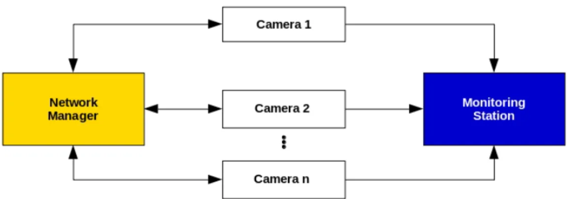
The system consists of a set of n cameras C = {c1, c2, ...cn} streaming to a monitoring station and providing information frame size to the network manager. This one distributes the global system’s bandwidth H dynamically among the cameras and performs admission control, as shown in figure3.1.

The cameras, when connecting to the system, request a channel to the manager and receive the initial image and bandwidth parameters values. After returning a positive response containing the value for the channel bandwidth, the manager sets up each camera’s channel and then requests a video stream for control and another video stream for the monitoring station for visualization.

At run time, the manager periodically checks the system’s needs, calculates new bandwidth values and reassigns them to the cameras. In parallel, at each frame, the cameras check the error between the assigned bandwidth and the bandwidth corresponding to the actual frame size and adapt the compression level accordingly. Each of the system’s modules will be described in detail in the next subsections.

3.2.1 Camera

Each camera captures a stream of images, encodes each image in a corresponding frame using codecs and then transmits the frames to the monitoring station. Defining the stream as Ic = {ic,1, ic,2, ...ic,m}, in which c identifies the camera and m is the number of images that are part of the stream, each element ic,pin this set, p ∈ {1, 2, ...m}, will have the following characteristics: • A quality qc,pthat represents, loosely, the percentage of information preserved after

3.2 System architecture 13

Figure 3.1: System’s functional architecture

• A size sc,prepresenting the image size after encoding and is comprised between sp,min and

sp,max; these values depend on hardware features (e.g., images resolution) and the codec

type.

The relationship between sc,p and qc,pis not linear, since it depends on many factors such as the complexity of the scene, the sensor used by the camera and the amount of light that reaches the sensor. This was explored in previous work ([9,10]) but, it will not be detailed in this dissertation since it is outside our specific methodology.

The camera adapts the parameter qc,pto make sc,pmatch the size corresponding to the target frame size Sctaking as input the normalized error between the two,

ec,p=

Sc− sc,p Sc

(3.1) and feeding it to a PI controller, which is described by the following equation:

q∗_c,p= Kp· ep+ Ki· p−1

∑

j=1

ec,i (3.2)

The raw value obtained is then bounded to the limits defined for this parameter,

qc,p= max(15, min(100, q∗c,p)) (3.3) We consider 15 the minimum value since it is the lowest level to provide a reasonable image. Finally, the compression level is set as 100 − qc,p.

3.2.2 Network Manager

The network manager performs admission control and periodic bandwidth redistribution. The first is responsible for creating the virtual channel for each camera that connects to the system, as explained above, and the second is responsible for modulating it periodically to fit the camera’s needs.

14 Methodology and system architecture

The bandwidth redistribution divides the global system’s bandwidth H dynamically among the cameras, allocating a fraction bcto camera c. This implies that,

n

∑

c=1

bc= 1 (3.4)

Regarding each camera, the fraction bc sets the value of allocated bandwidth Bc given by

Bc= bc· H (3.5)

and, knowing frame rate τc, it also sets the value of the target frame size for camera c,

Sc= bc· H

τc

(3.6) To define bc for all cameras we used the game-theoretic approach described in [12]. The control is described by the following equation:

bc,t+1= bc,t+ ε · [−λc· fc,t+ bc,t· n

∑

i=1

(λi· fi,t)] (3.7) Note that bp,t+1is the bandwidth fraction that will be allocated to camera c in the next manager control interval [t,t + 1], bc,t is the allocated bandwidth fraction in the previous manager interval control [t − 1,t] and fc,t is the so-called the matching function, which represents to what extent the amount of network bandwidth allocated to camera c at the instant t is a good fit for the current quality.

Besides these parameters directly related to the cameras’ QoS, there are two more that influ-ence the amount of bandwidth allocated in each manager iteration: ε and λc. The first one affects the responsiveness and stability of the system. Higher values will provide faster convergence in trade for some overshooting, while lower values slow down the convergence but increase the ro-bustness in case of sporadic disturbances. The second one, represents how much the manager is willing to allocate bandwidth to camera c. Higher values relatively to the other cameras will make the manager favour camera c, while lower values will do exactly the opposite.

As matching function, similarly to [12], we use the normalized error between frame size and the target frame size for camera c, where p is the latest frame of camera c at the manager iteration t:

fc,t=

Sc− sc,p Sc

(3.8) Proof of convergence of this method is presented in [12].

3.2.3 Quality equalization among cameras

Although the solution for bandwidth distribution proposed by [12] has been proven to provide an efficient bandwidth control, it has limitations in what regards to quality equalization. As we

3.2 System architecture 15

will see later in chapter 5, if the system starts with only one camera seeing a simple scenario and a second camera, seeing a complex scenario, joins the system, it would be expected that the system would redistribute the bandwidth, providing a bigger share to the second camera, so it could have a reasonable image quality. However, since with Linux TC we cannot initialize a camera’s bandwidth with zero when it joins the system - which excludes all types of communication - we must allocate a low value to reduce its impact in the system when joining. If the quality is also initialized with a low value for the same reason, what will happen is that the error will be quickly compensated with low QoS, stabilizing with a complex image with low quality.

Since one of the objectives of this project is to have a system capable of equalizing the quality of all cameras that are not in focus - we consider "in focus" a camera temporarily selected by an operator to have more quality than the other ones - we created a factor, that we named quality balance (Ccfor camera c), and that is added to the bandwidth fraction resulting from each network manager iteration in order to accomplish this equalization. This factor is based on qdev_c,t , the nor-malized deviation of camera c from the average quality of all cameras ¯qt at instant t, and has a different behaviour depending on whether qdev_c,t is greater or lower than zero.

Initially, we developed this factor making it depend on the value of λcand defining it as

Cc=    −α · (qdev c,t · λc)3, if qdevp ≤ 0 −β · (qdev c,t · (1 − λc))3, otherwise with qdev_c,t given by

qdev_c,t =qc,t− ¯qt ¯ qt

(3.9) and α and β being coefficients that define the speed of compensation, are set up offline and must always have positive values. The cubic exponent is explained by the initial behavior thought for the factor: positive compensation for negative quality deviations and negative compensation for positive quality deviations, with null derivative at zero deviation. However, since we wanted a different compensation speed in each situation, we decided to divide the factor in two branches.

The quality balance factor was added to the raw result from the bandwidth controller and was used in the first four experiments that we show in Chapter5. However, we decided to create a quality gain (Gc for camera c), that would determine the behavior of the quality balance factor, ensuring a balanced resource utilization. This way, the quality balance factor would not depend on or affect other factors also depending on λ . Thus, the function was redesigned as follows to smooth the impact caused by Gcchanges:

Cc=    −α · Gc· (qdevc,t )3, if qdevc,t ≤ 0 −β · (1 − Gc) · (qdevc,t )3, otherwise

Gc is a configuration parameter that can be adjusted by the user at any time, for example using a control panel, with the purpose of accelerating or slowing the compensation for a certain

16 Methodology and system architecture

camera when it is above or below average quality. Internally, the network manager enforces a normalization of the quality gains as follows:

n

∑

c=1

Gc= 1 (3.10)

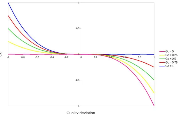
Figure3.2 shows the variation of Cc depending on qdev_c,t and Gc with α = 1 and β = 1. We can see that, given 0 ≤ Gc ≤ 1, Cc will always be positive if qdevc,t < 0 and negative otherwise, effectively contributing to balance camera qualities.

Figure 3.2: Compression compensation vs. qdev_c,t for multiple values of Gc

When the quality gain is Gc= 0.5 the quality balance factor Cc becomes symmetrical with respect to the quality deviation qdev_c,t . This means the compensation will be the same in magnitude, whether the quality is lower or higher than the average. In the range 0 ≤ Gc≤ 0.5 the compensation will be stronger when the qualities are higher than average and lower otherwise. Conversely, the range 0.5 ≤ Gc≤ 1 leads to stronger compensations when the quality is below average.

When in an unbalanced situation, having a quality above average means that the respective camera has more capacity to reduce its bandwidth than the other ones. In other words, such camera has higher bandwidth than needed and it is potentially contributing to overrun the system bandwidth. Thus, it makes sense to increase the magnitude of the compensation when the qual-ity deviation is positive (qdev_c,t > 0). This is naturally enforced by the normalization of the quality gains. As more cameras are added, the gains will tend to smaller values promoting stronger com-pensations for positive quality deviations than for negative deviations.

Chapter 4

Implementation

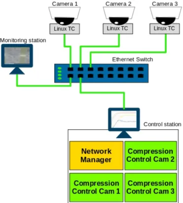
This chapter describes the implementation of the system, detailing the evolution of the process and the technologies used. The system hardware architecture is shown in figure4.1

4.1

Cameras

The cameras available in the lab are Axis Communications professional surveillance cameras, models P5512 and P5512-E PTZ. Thus, we started by exploring their features in order to see how they could be useful for the purposes of our project.

4.1.1 Parameter setup

One of the most important features to communicate with the cameras is its embedded HTTP server. Together with the API VAPIX®[28], developed by Axis Communications, most of the cameras’ parameters can be viewed and changed remotely through common HTTP GET and POST requests. For example, to request an MJPEG stream or change the compression parameter:

MJPEG Stream: http://«hostname»/axis-cgi/mjpg/video.cgi (GET) Compression: http://«hostname»/axis-cgi/param.cgi?action=update&

Image.I0.Appearance.Compression=«value» (POST) The parameters can also be changed using the web application that comes with the cameras, which also allows controlling the cameras’ Pan, Tilt and Zoom (PTZ).

4.1.2 Rate control

These cameras include control mechanisms to offer CBR (for H.264) and Maximum Frame Size (for MJPEG), which, in the beginning, seemed like nice features to use advantageously to the project and maybe avoid the use of Linux TC. However, the cameras would not return the in-stantaneous compression value thus not allowing the compensation by increasing the allocated

18 Implementation

Figure 4.1: System’s implementation

bandwidth in case the compression was too high or too low. This defined the strategy of develop-ing the compression control module that is described in4.2.1.

The fact that the cameras are Linux-based opened the door for using Linux TC directly in the camera instead of having an external computer post-processing the stream. This was pos-sible through establishing an SSH connection with each camera and sending the configuration commands directly. The Linux distribution embedded in the cameras did not allow for complex configurations, though. Ideally, a PRIO qdisc would be used, together with a filter, in order to give priority to the control traffic and then forward the video traffic to a Token Bucket Filter (TBF) so it could be shaped to the desired bandwidth. Since the camera did not support the PRIO qdisc, neither any other classful qdisc, and taking into account that the control traffic would be low comparing to the stream traffic, the final decision was to go only with the TBF, reserving some bandwidth for the control traffic in the network manager calculations.

TBF consists, basically, in the CPU generating tokens at a defined rate, which are kept in a bucket. The size of the bucket is user defined and must be carefully calculated in order to ensure the desired rate. The tokens roughly correspond to authorizations to send bytes. As long as there are tokens available in the bucket, data can be sent by the network interface and every time data is actually transmitted, the corresponding tokens are deduced from the bucket. When the bucket runs out of tokens, the data is queued, waiting for tokens, until the defined latency or limit is reached. In that case, the data is discarded.

4.2 Control Station 19

The Linux TC was configured for using TBF with the following command: tc qdisc replace dev eth0 handle 1: root tbf rate <rate> burst <burst>

[latency <latency> | limit <limit>]

In this command, <rate> is the bandwidth value allocated by the network manager, <burst> is the amount of data that can be transmitted in one second and latency was set to zero since queuing packets would lead to undesired streaming delays.

4.1.3 Streaming

The cameras can stream using two different protocols, HTTP and RTSP, both having the possibility to be requested via VAPIX®. Using RTSP over UDP would, in principle, be the best solution for streaming efficiently and with low overhead. Unfortunately, if the image parameters are changed, the RTSP session must be restarted to get a stream with the updated parameters. Since the control would be done frame by frame, and, to be started, each session needs three requests - DESCRIBE, SETUP, PLAY - this protocol would impose significant overhead, eventually causing many frames to be dropped. This limitation also affects the streaming through HTTP over TCP but we chose it because it takes only one message to be restarted, and it allows the control to get the frame size at the first frame packet, while with RTSP, the controller would need to receive the whole frame.

4.2

Control Station

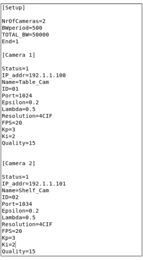
The control station runs all the compression control modules that are part of the system, exchang-ing all the information needed with the cameras. The programmexchang-ing language chosen to implement them was C, using libcurl [29] and the available examples for implementing the communication with the cameras through HTTP requests. We used a key file to set the initial value for most of the system’s parameters. The file structure is shown in figure4.2.

4.2.1 Compression control

Initially we tried implementing the compression control module in the camera. This way, the control could be faster since it would not require any external communication as in [12]. However, this idea was dropped because the development tools for the computers embedded in the cameras were no longer available.

Therefore, we decided to implement the compression control in the same computer as the Network Manager, one independent controller per camera. For each camera, two threads were created: one for receiving the respective stream and another for this control. The first thread checks every packet received for the word "Length" present in the HTTP header data, which indicates the size of the next frame to be transmitted. When found, this thread signals the compression control thread and interrupts the stream so that it can restart it after the new compression parameter is set. The streaming is a multi-part HTTP request which continues as long as the camera is transmitting

20 Implementation

Figure 4.2: Parameters file

images or until the receiver returns a number different from the number of bytes received. In this case, e.g., when the callback function receiveStream returns −1, the streaming is interrupted (see SectionA.1in the Appendix). After being signaled, the compression control thread gets the frame size, performs the calculations described in3.2.1, executes the appropriate HTTP request to change the compression for the new value and signals the streaming thread to restart the stream. To prevent the integrator from overflowing the output, an anti-windup mechanism was implemented (see the code in AnnexA).

4.2.2 Network Manager

As previously mentioned, the Network Manager comprises the admission control and the band-width distribution modules. The cameras have a Bonjour server (Apple’s implementation of Ze-roConf). This allows devices to advertise their services and be discovered in the network without having an IP within the network range and would be a useful feature to help implementing admis-sion control. Unfortunately, there was no time to explore this possibility and thus the admisadmis-sion control was implemented based on the parameters file referred before to acknowledge the cameras connection to the system. The file key "NrOfCameras" is checked each second for changes. If a

4.2 Control Station 21

change is detected, the module will read the key "Status" of each "Camera x" field to check what changed and (dis)connect the cameras accordingly.

As for the bandwidth distribution, one of the questions that has arisen when thinking about the implementation was about making it synchronous or asynchronous. Since Linux TC can be reconfigured at any time, it provided the possibility of an asynchronous implementation. This would bring some complex issues to consider, though. Being the initial idea implementing the control modules in separate devices, a standard communication architecture, such as Master-Slave or Client-Server, would not be enough. Since all devices would need to send renegotiation requests to the manager and listening at the same time for eventual updates already being done, this would bring some unpredictability to the control and would require a more complex implementation to establish minimum quality requirements for each camera at any instant and avoid race conditions. Having in mind building a system comparable with others from previous work, and given the time available, we decided to implement a synchronous network manager, with a user-defined period, π .

The bandwidth distribution module gets the frame size from the camera and the quality values from the compression control modules and performs the calculations described in3.2.2. The result is constrained to the interval [0.1 0.9] to avoid allocating the whole bandwidth to a single camera while guaranteeing a minimum value, and is then multiplied by two and used to set the bandwidth reservation and build the respective Linux TC command, which is then sent through SSH [30]. The reason why it is multiplied by two is due to the cameras transmitting two simultaneous streams: one for compression control and one for monitoring (display station). Thus, we are using twice the bandwidth that would be effectively needed if the compression control was carried out inside the cameras but it was a practical way to circumvent the limitations of the actual cameras available for this project. On the other hand, the compression control uses just the control stream, thus only half of the bandwidth reserved in the respective camera. This value, i.e., half of the reserved bandwidth, is adjusted to remove the estimated control overhead and used to compute the target frame size and in further calculations (see the code in AnnexA.3).

The value for the overhead was defined based on observations using Wireshark. From these observations, we derived the maximum packet payload for stream packets (MP = 1448 Bytes), the stream control overhead (SC = 132 Bytes per frame, including headers and ACK messages), the SSH messages (SSH = 694 Bytes per Network Manager iteration) and the compression setting (CS = 600 Bytes per compression control iteration) and added an offset due to frame size variations (OF = 1500 Bytes). This resulted in the following total overhead per frame calculations:

Total_Overhead_ f rame = (sc,p/MP + 1) ∗ SC +CS + OF+ +SSH·

1 π τc

Chapter 5

Experimental Validation

This chapter presents the system experimental validation in which we used three cameras: two P5512-E and one P5512. The cameras have a feature that allows to save several positions in order to make quick transitions. For example, after positioning the cameras, we pointed them to a certain scenario, using the PTZ control, and saved that position using a name (e.g. Complex scenario). After planning the scenarios needed for the experiments, this mechanism was used to save these positions, guaranteeing that the transitions were quick and stable and that the same scenarios would be used for all experiments in order to get coherent results. The devices were connected through a switch, similarly to figure4.1. To validate our system we carried out 5 experiments:

Experiment 1: A camera is given a fixed bandwidth and, at some point, the image is changed so the compression adaptation mechanism can be observed.

Experiment 2: The system starts with only one camera. At some point, another camera capturing a similar image joins the system so the bandwidth redistribution can be observed.

Experiments 3 and 4: One camera sees a complex image and the other sees a simple one. The system starts with one of the cameras and, at some point, the other joins.

Experiment 5: The system starts with camera 1 only and the others join the system sepa-rately in the course of the experiment.

In all experiments, when the system starts, the global bandwidth is equally distributed through all the connected cameras. If some camera joins the system during run time, a low value (800Kbit/s) is allocated to reduce the impact on the cameras already connected and let the system then evolve according to the needs of all the cameras. The values set for all parameters in each experiment are shown in table5.1.

The values for ε, λ , π, α and β were chosen based on several experiments performed to find the values that provided stability and effectiveness to the system. Since the number of cameras increased in experiment 5, the previously used value for λ was too high and caused instability as the system was doing a great effort trying to compensate all cameras with a high bandwidth

24 Experimental Validation

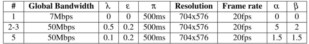
Table 5.1: Parameter values in each experiment

# Global Bandwidth λ ε π Resolution Frame rate α β

1 7Mbps 0 0 500ms 704x576 20fps 0 0

2-3 50Mbps 0.5 0.2 500ms 704x576 20fps 5 2 5 50Mbps 0.1 0.2 500ms 704x576 20fps 1.5 1.5

fraction. Therefore, we decreased the value of λ . The values for α and β were changed in the last experiment due to the use of the new Gcfunction referred in3.2.3.

It is worth noting that, as the cameras need the stream to be restarted each time its compression value is changed, this introduces delays in the control thus reducing the frequency of the control iterations from its ideal value, τ, to a maximum of 8 iterations per second. Several experiments were conducted to evaluate if this frequency would be higher at lower frame rates, but the maxi-mum obtained was always 8. However, this did not have a significant impact in the controller as we will see in the next sections.

5.1

Experiment 1

In this experiment, a camera was pointed at a simple scenario and, between t = 30 and 40 seconds, the image was changed to a more complex scenario. We used a low value for the global bandwidth so the controller would need some effort to adapt. Figure5.1shows the two images captured by the camera.

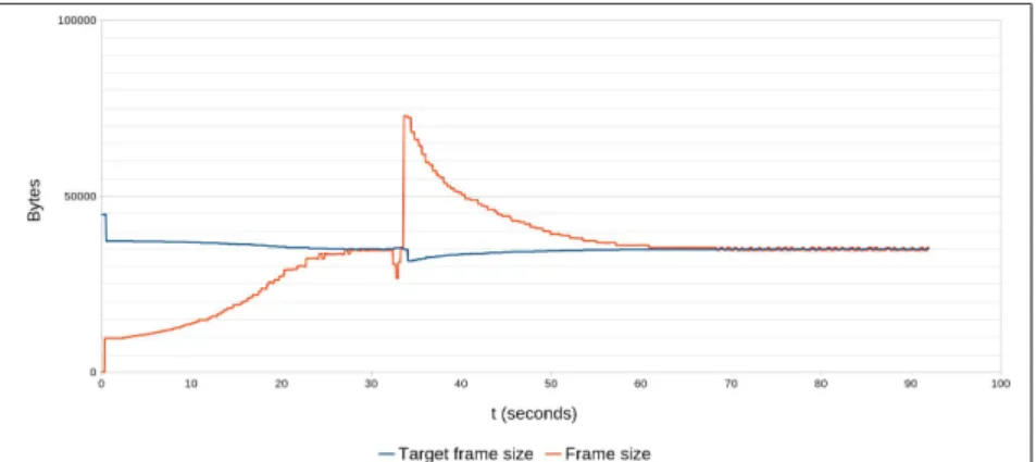
Figures5.2 and 5.3 show that the bandwidth allocated to the camera is constant during the whole experiment, except for the initial drop down resulting from the bounding mechanism men-tioned in4.2.2. The camera starts pointed at Scenario 1 and, at t ≈ 34s, the camera switches to Scenario 2 and the compression control immediately starts increasing compression, decreasing the frame size and the quality of the image, stabilizing at t ≈ 70s. We can see that the real frame size exceeds the target frame size significantly when the scenario changes. However, this does not mean that the camera uses more bandwidth than what was allocated. The frame generation system is totally independent from the Linux TC, which means that, although the generated frame size is higher than the bandwidth allocated, the amount of data transmitted will never exceed this value. This means that, between t ≈ 34s until the setpoint is reached again, some frames are lost.

5.2

Experiment 2

In this experiment, two cameras were capturing similar scenarios, as shown in figure 5.4. The system starts with camera 1 only and, at t ≈ 39s, camera 2 joins the system.

In figure5.5 we can observe that, when camera 2 joins, some over and undershoot can be seen in the bandwidth distribution but, after approximately 5 seconds, it stabilizes, with camera 1 returning to the same value as before and camera 2 being allocated some of the spare bandwidth.

5.2 Experiment 2 25

Figure 5.1: Experiment 1 scenarios: Scenario 1 (Left) and Scenario 2 (Right)

Figure 5.2: Experiment 1: Quality and bandwidth when changing the complexity of the image of a single camera

Figure 5.3: Experiment 1: Target frame size versus actual frame size size when changing the complexity of the image with a single camera

26 Experimental Validation

At this point, the compression balance factor starts its work, slowly adapting the bandwidth of both cameras to equalize the quality of both.

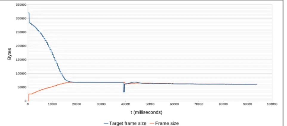
In figures5.6and5.7, the matching of the bandwidth allocated to the frame size of cameras 1 and 2, respectively, can be observed. Note that the scales are different to provide a better visual-ization of the whole experiment. We can see that, after the system stabilizes, the target frame size and the actual camera frame size follow each other closely, which shows the effectiveness of the network manager.

Figure 5.4: Experiment 2: Camera 1 starts seeing the image on the left and at time 40s camera 2 joins seeing a similar image (right)

Figure 5.5: Experiment 2: evolution when a second camera joins at t ≈ 39s, both seeing a similar image

One observation that can be made is that, although camera 1, at the start, and camera 2 when it joins, have much bandwidth available, their quality is not maximized. This happens due to the times of actuation of both controllers. Since at the first iteration of the bandwidth distribution, the value for quality is too low, it adapts to that value, reducing the bandwidth requirements.

5.3 Experiments 3 and 4 27

Given this situation, when the error is compensated, the bandwidth allocated is already low so the compression controller stabilizes according to this value. This behaviour could be compensated setting a higher initial quality value, so the difference would not be so significant or setting a more adequate value for λ in each case, and, perhaps, varying it during the process, to take the most of the compression controller.

Figure 5.6: Experiment 2: Allocated target frame size vs. actual frame size from camera 1

Figure 5.7: Experiment 2: Allocated target frame size vs. actual frame size of camera 2

5.3

Experiments 3 and 4

In these experiments, one camera was pointed at a complex scenario (scenario 1) and the other one was pointed to a simple scenario (scenario 2), both shown in Figure5.8.

Experiment 3 started with camera 1 pointed at scenario 2 and after 44 seconds, camera 2, which was pointed at scenario 1, joined the system. In experiment 4, the scenarios were switched between the cameras. These experiments were analyzed together in order to compare how the system reacts depending on the complexity of the scenario being captured by the joining cameras.

28 Experimental Validation

Figure 5.8: Experiments 3 and 4 scenarios: Scenario 1 (Left) and Scenario 2 (Right)

Figure 5.9: Experiment 3: Quality and bandwidth evolution when a camera joins with more complex images

5.4 Experiment 5 29

Figure 5.10: Experiment 4: Quality and bandwidth evolution when a camera joins with more simple images

From both results we can conclude that, when a camera joins with a simpler scenario than the scenario of another camera already in the system, the network manager tends to compensate the one pointed at the complex scenario more significantly than when the opposite happens. This is due to the same behaviour observed in figure5.2regarding the camera’s start conditions.

5.4

Experiment 5

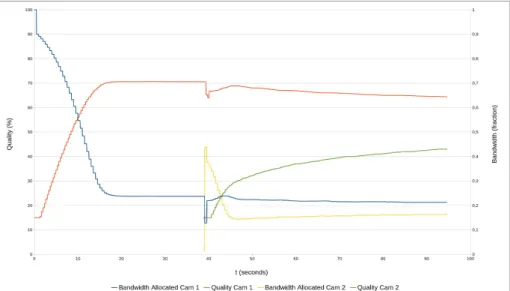
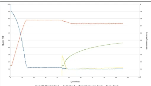
In this experiment, the system starts with camera 1 only. At t ≈ 44s camera 2 joins and, at t ≈ 102s, camera 3 joins. Figure5.11shows the scenarios used. This experiment approximates the application of this system in a real video surveillance system, with several cameras, joining at different instants. Figures5.12and5.13show the results.

Figure 5.11: Experiment 5 scenarios: Camera 1 (Left), Camera 2 (Middle) and Camera 3 (Right)

For t ∈ [0, 44]s, the system starts allocating the necessary resources to camera 1, which stabi-lizes at approximately t ≈ 18s. In this time interval, the Quality Gain is not relevant since there is

30 Experimental Validation

only one camera and thus, the quality deviation is always zero.

At t ≈ 44s, camera 2 joins, and we can see some overshoot and undershoot in the bandwidth allocation, reaching saturation. This was due to the fact that, although in this experiment the value chosen for lambda was low, the values chosen for α and β were still too high. Anyway, the network manager recovers, and the cameras start to stabilize, with the effect of Cc making the qualities converge to the average, as can be seen between 60s and 102s.

At t ≈ 102s, camera 3 joins, also overshooting, but, right after, Ccstarts compensating that and equalizing the qualities of all cameras.

Figure 5.12: Experiment 5: Quality evolution when 2 cameras join at different instants and the quality gain is changed

Figure 5.13: Experiment 5: Bandwidth evolution when 2 cameras join at different instants and the quality gain is changed

5.4 Experiment 5 31