Deep Learning for the Segmentation of Vessels in Retinal Fundus images and its Interpretation

F

E

U

P

Deep Learning for the Segmentation of

Vessels in Retinal Fundus images and its

Interpretation

Pedro Filipe Cavaleiro Breda

Mestrado Integrado em Engenharia Eletrotécnica e de Computadores Supervisor: Hélder Filipe Pinto de Oliveira, PhD

Second Supervisor: Ricardo Jorge Terroso de Araújo, MSc

c

Abstract

Vessel segmentation is a key step for various medical applications, it is widely used in monitoring the disease progression, and evaluation of various ophthalmologic diseases. However, manual vessel segmentation by trained specialists is a repetitive and time-consuming task. In the last two decades, many approaches have been introduced to segment the retinal vessels automatically.

With the more recent advances in the field of neural networks and deep learning, multiple methods have been implemented with focus on the segmentation and delineation of the blood vessels.

Deep Learning methods, such as the Convolutional Neural Networks (CNN), have recently become one of the new trends in the Computer Vision area. Their ability to find strong spatially local correlations in the data at different abstraction levels allows them to learn a set of filters that are useful to correctly segment the data, when given a labeled training set.

In this dissertation, different approaches based on deep learning techniques for the segmen-tation of retinal blood vessels are studied. Furthermore, in this dissersegmen-tation are also studied and evaluated the different techniques that have been used for vessel segmentation, based on machine learning (Random Forests and Support vector machine algorithms), and how these can be com-bined with the deep learning approaches.

Acknowledgements

In first place I would like to thank professor Helder Oliveira, my supervisor, for the guidance and follow-up of the work done and the opportunity to work at INESC TEC. Furthermore, I can’t express my gratitude for the support and comprehension regarding all of the problems and setbacks that prevented the conclusion of this dissertation during the required period. His support and comprehension were key to no give up on all the work done over the last months, and for that I will be always thankful.

The biggest thanks to Ricardo Araújo, for being the co-supervisors every student hopes for and even more, and for everything: the help since day one with the review of the literature and research, the willingness to help on every aspect of the work, from providing code samples to the correction and review of this dissertation. Without you, this dissertation would not be half of what it is. To Ricardo, I would also like thank the support and comprehension with situation previously described and apologize of every inconvenient that it may caused to his work.

To my mother, the greatest thanks of all, for all help and the support during this long and difficult journey, in particular these last months. You made unthinkable efforts to make this journey possible, remanding me every step of the way that I had all the capabilities to be whatever I wanted to be. All of your sacrifices allowed me to prose the key aspects for personal growth, which is education, and for that i would be forever grateful.

Also I would like to thank the rest of my family and friends, in special to Ana Beatriz for the support and help dealing with everything in the past couple of months, and to my roommate Pedro Cardão for offering his personal computer setup to run some of the implementations.

Pedro Breda

“Agir, eis a inteligência verdadeira.”

Fernando Pessoa

Contents

2.1.1 Retinal layer & structure . . . 4

2.1.2 Vessels and Blood supply of the retina . . . 5

2.2 FundusImage . . . 6

2.3 Databases . . . 8

2.3.1 DRIVE Database . . . 8

2.3.2 STARE Database . . . 9

3 State of the art 10 3.1 Performance Indicators . . . 11

3.2 Unsupervised Learning and other approaches . . . 12

3.2.1 Unsupervised Learning . . . 12 3.2.2 Matched Filtering . . . 12 3.2.3 Morphological Processing . . . 13 3.2.4 Vessel Tracing/Tracking . . . 14 3.2.5 Multi-scale approaches . . . 14 3.3 Supervised methods . . . 15

3.3.1 Traditional Machine learning . . . 15

3.3.2 Deep Learning . . . 17

3.4 Summary and Comparison . . . 25

4 Methodology 27 4.1 Data preparation . . . 28

4.1.1 Image Pre processing . . . 28

4.1.2 Division into patches, data normalization and standardization . . . 28

4.2 Convolutional neural networks for retinal vessel segmentation . . . 32

4.2.1 Patch Classification approach . . . 32

4.2.2 Patch Segmentation approach . . . 37

4.3 Convolutional neural networks for deep features extraction . . . 39

4.3.1 Feature extraction . . . 40

4.3.2 Classifiers . . . 40 vii

viii CONTENTS

4.3.3 Ensemble . . . 43

5 Results and Discussion 45 5.1 Results of CNN based approaches for retinal vessel segmentation . . . 45

5.1.1 Patch Classification approach . . . 45

5.1.2 Patch Segmentation approach . . . 49

5.2 Results of CNN for deep feature extraction . . . 51

5.2.1 Random Forests . . . 51

5.2.2 Support Vector Machines . . . 53

6 Conclusions and Future work 54 6.1 Conclusions . . . 54

6.2 Future Work . . . 55

A Tables of results 57 A.1 Results of CNN Based approaches for retinal vessel segmentation . . . 57

A.1.1 Results of the Melinscak based approach . . . 57

A.1.2 Results of Liskowski based approachs . . . 58

A.2 Results of CNN for deep feature extraction approaches . . . 63

List of Figures

2.1 Representation of the structures involved in fine vision [7]. . . 4

2.2 Schematic representation of the choroidal circulation [11]. . . 5

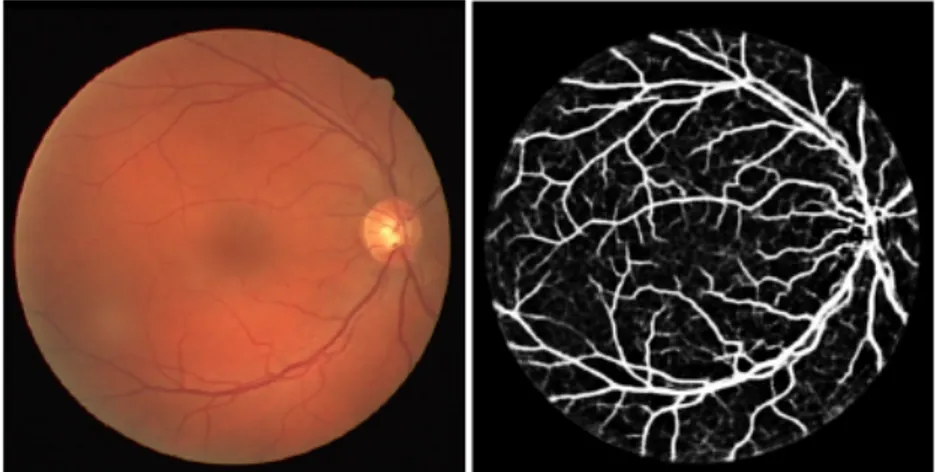
2.3 FundusFluorescein Angiography illustrating the retinal circulation [12]. . . 6

2.4 Examples of fundus photography using 40◦, 20◦and 60◦FOV [13]. . . 7

2.5 Original DRIVE image (a), it’s manual segmentation (b) and binary mask (c). . . 8

2.6 Original STARE image (a), it’s manual segmentation (b) and binary mask (c). . . 9

3.1 Example of a line detector with its orthogonal line as implemented by Ricci et al. [41]. . . 16

3.2 Schematic representation of the Convolutional Neural Network presented by Wang et al.[44]. . . 19

3.3 Structure of the proposed method by Wang et al. [44]. . . 19

3.4 Best accuracy results obtained by Wang et al. [44] on DRIVE image. . . 20

3.5 Best result of the best AUC score and Softmax activation obtained by Melinscak et al. [48]. . . 21

3.6 Network architecture for edge detection using HED [50]. . . 22

3.7 Structure of the proposed method by Fu et al [49]. . . 22

3.8 Example of Training patches after applying GCN transformation [51]. . . 24

3.9 Example of Training patches after applying ZCA whitening transformation [51]. . 24

3.10 Example of Training patches using data augmentation [51]. . . 24

3.11 Ground truth (left) and segmentation result (right) for two healthy subjects: (a) DRIVE and (b) STARE [51]. . . 24

4.1 Overall image pre-processing stages. . . 29

4.2 Example of a positive set of patches (a) and a negative set of patches (b). . . 30

4.3 Original patches (left) and respective data augmentation transformation results (right). . . 31

4.4 Example of the architecture of a classic Neural Network [55] . . . 32

4.5 Equations used during the application of batch normalization layer [66] . . . 34

4.6 Illustration of the dropout process. On the left is an example of the standard pro-cedure and on the right is the result of the Dropout [67]. . . 34

4.7 A training example for the SP approach: the 27x27 patch (left) with a s x s = 5 x 5 and the corresponding desired output (right) [51]. . . 37

4.8 Example with the schematics and description of a U-net architecture with the iden-tification of the contracting and expanding paths [65]. . . 38

4.9 Example of features extracted from (a) MP01 layer and from MP02 (b). . . 41 4.10 Illustration of how the random forest algorithm preforms a classification task [70]. 41

x LIST OF FIGURES

5.1 Original DRIVE image (a), its manual segmentation (b) and Best overall result of the Melinscak based approach on the DRIVE dataset (c). . . 46 5.2 Original STARE image (a), its manual segmentation (b) and Best overall result of

the Melinscak based approach on the STRARE dataset (c). . . 46 5.3 Original DRIVE image (a), its manual segmentation (b) and Best overall result of

the Liskowski SP based approach on DRIVE dataset (c). . . 47 5.4 Original DRIVE image (a), its manual segmentation (b) and Best overall result of

the Liskowski Random based approach on DRIVE dataset (c). . . 48 5.5 Original DRIVE image (a), its manual segmentation (b) and Best overall result of

the Liskowski Random based approach on DRIVE dataset (c). . . 48 5.6 Original DRIVE image (a), its manual segmentation (b) and Best overall result of

the U-Net based approach on DRIVE dataset. (c). . . 50 5.7 Original STARE image (a), its manual segmentation (b) and Best overall result of

the U-Net based approach on STARE dataset. (c). . . 50 5.8 Original DRIVE image (a), its manual segmentation (b) and Best overall result of

CNN and Random Forest classifiers of this approach on DRIVE dataset (c). . . . 52 5.9 Original DRIVE image (a), its manual segmentation (b) and Best ensemble result

List of Tables

3.1 Vessel classification. . . 11

3.2 Performance indicators and metrics for vessel segmentation. . . 11

3.3 Architecture of the implemented Convolutional Neural Network by Wang et al. [44]. 19 3.4 Architecture of the implemented Convolutional Neural Network by Melinscak et al.[48]. . . 20

3.5 Two most relevant architectures proposed by Liskowski and Krawiec [51]. . . 23

3.6 Performance analysis of the methods presented in Chapter 3. . . 26

4.1 Architecture of the implemented Convolutional Neural Network. . . 35

4.2 Architecture of the implemented Convolutional Neural Network based on the ap-proach proposed by Liskowski. . . 36

4.3 Structure of the implemented U-Net. . . 39

4.4 Structure of the LeNet used for feature extraction. . . 40

5.1 Average results of the Liskowski based implementations on the DRIVE dataset. . 47

5.2 Average results of the Liskowski based implementations on the STARE dataset. . 48

5.3 Average results of the U-net implementation on DRIVE and STARE datasets. . . 49

5.4 Average results of CNN, Random Forest Classifiers and Ensemble mechanism obtained on DRIVE dataset. . . 51

5.5 Average results of CNN and the different SVM classifiers used obtained on DRIVE dataset. . . 53

A.1 Results of the Melinscak based approach tested and trained on DRIVE dataset . 57 A.2 Results of the Melinscak based approach tested and trained on STARE dataset . 58 A.3 Results of the Liskowski based approach Trained on DRIVE dataset . . . 58

A.4 Results of the Liskowski based approach trained using balanced data on DRIVE dataset . . . 59

A.5 Results of the Liskowski based approach trained using random data on DRIVE dataset . . . 60

A.6 Results of the Liskowski based approach trained on RGB data From DRIVE dataset . . . 61

A.7 Results of the Liskowski based approach trained on STARE dataset . . . 61

A.8 Results of the Liskowski based approach trained using balanced data on STARE dataset . . . 61

A.9 Results of the Liskowski based approach trained using random data on STARE dataset . . . 62

A.10 Results of the Liskowski based approach trained using RGB Data from STARE dataset . . . 62

A.11 Results of CNN used for feature extraction trained on DRIVE dataset . . . 63 xi

xii LIST OF TABLES

A.12 Complete results from the CNN. Random Forest classifiers and ensemble mecha-nism on DRIVE dataset. . . 64

Abbreviations

2D Two dimensional 3D Three dimensional ACC Accuracy

AUC Area under the operating Characteristic curve CNN Convolutional Neural Network

FOV Field of View FP False Posite FN False Negative FPR False Positve Rate ReLu Rectified linear unit RF Random Forest Classifier SN Sensitivity

SP Specificity

SVM Support Vector Machines TP True Possitive

TN True Negative TPR True Positive Rate

Chapter 1

Introduction

1.1

Context

The retina is a layered tissue coating the interior of the eye responsible for the formation of images, that is, for the sense of vision. By allowing the conversion of light into a neural signal that will be later processed in brain visual cortex, this anatomic structure is one of the most important for the wellbeing of the human individual [1]. As result of its function, the retinal tissue is classified as highly metabolically active, having a double blood supply which allows a direct non-invasive observation of the circulation system [1].

During the last 160 years, retinal imaging has grown rapidly and is now one of the most common practices in clinical care and patient monitoring for people suffering from retinal and/or systemic diseases. The fundus photography technique is used in large scale detection of diabetic retinopathy, glaucoma and age-related macular degeneration [2] .

With the more recent advances in the field of neural networks and deep learning, multiple methods have been implemented with focus on the segmentation and delineation of the blood vessels. Each approach attempts to identify and organize the fundus image according to a set of features and with that recognize the vessel structure, fovea, macula and the optic disc [3].

The different types of networks, as well as the different types of data available, allows the implementation of a new and improved solution, which can be compared with the previous work done in this area [4].

For this thesis, one goal is to study the result of different combinations of neural networks tested and trained in different databases and do a comparative analysis with other solutions avail-able, considering not only deep approaches for this regard. With this study complete and serving as support, we will attempt to implement a solution, or a set of solutions to automatically segment the retinal blood vessels. The results of the presented solution will then be analyzed, interpreted and benchmarked with the available ones.

2 Introduction

1.2

Motivation

Automatic segmentation of vessels in 2D and 3D data is a task that has been already addressed by several researchers. This comes from the importance that these structures have when considering the evaluation of different pathological conditions, such as diabetic retinopathy in retinal fundus images, and coronary artery disease in cardiac data. Often, the experts have too much data to analyse, leading to the necessity of having Computer Aided Detection tools that can accurately perform these tasks.

Many methods have been used to perform vessel segmentation. Convolution with matched filters is an important subset of that group. These filters are approximations to the local profiles that vessels are expected to have and their convolution with the data outputs higher values at the locations where the similarity is higher. Even then, it is common that vessels show different types of cross section profiles, making the a priori design of filters a complex task.

Deep Learning methods, such as the Convolutional Neural Networks (CNN), have recently become one of the new trends in the Computer Vision area. Their ability to find strong spatially local correlations in the data at different abstraction levels allows them to learn a set of filters that are useful to correctly segment the data, when given a labeled training set. Furthermore, analyzing the features that the CNN used to solve a task could be useful for humans to understand better the original problem.

1.3

Objectives

The main goal for this dissertation is to study and analyze different approaches based on deep learning techniques for the segmentation of retinal blood vessels. In order to do so, different design and architectures of CNN’s will be studied and analyzed, as their results and performance are evaluated and compared with the available algorithms.

One other important objective of this work is to study and evaluate the different techniques that have been used for vessel segmentation, based on machine learning, and how these can be com-bined with the deep learning approaches: by analyzing the features that the learned models are using to perform classification and combining them with different machine learning techniques, another objective is to propose a solution or set of solutions to perform the retinal vessel segmen-tation, using this methodology of work.

1.4

Document Structure

This document is divided into seven main sections. The presented section is the introduction to this dissertation. Chapter 2 is a brief description of some pertinent background information regarding the anatomic structure of the retina, its vessel structure and blood supply as well as the fundus photography technique. In this chapter both datasets used during the work are also described, detailing all the technical information regarding the image acquisitions and data format.

1.4 Document Structure 3

On chapter3the stat of the art of retinal vessel segmentations is presented, the methods studied are divided in unsupervised and supervised, and then subdivided according to the technique used. All of them are presented, analyzed and their results are then summarized and compared in the final of said chapter.

On the chapter4is presented the methodology of work, the proposed solution and its detailed implementation is described. The results obtained during the work, its analysis and discussion are presented on Chapter5. Lastly, on the final chapter (6) are discussed the conclusions and possible future work regarding the developed solution.

Chapter 2

Background

2.1

Anatomic structure of the retina

The retina is a light-sensitive tissue that exists inside the eye, behaving like a film in a camera. A series of chemical and electrical events occurs within the retina triggered by the optical elements of the eye as they focus an image. The electrical signals resulting from this chain of events are then sent to the brain via nerve fibers, where they are interpreted as visual images [5].

This structure, on human individuals, is located in the inner surface of the posterior two-thirds to three-quarters of the eye [6]. A thin, delicate, transparent sheet of tissue derived from the neuroectoderm, the retina comprises the sensory neurons, which is the beginning of the visual path way. Multiple neurons compose the neural retina (neuroretina). The neural retina is divided into nine layers and is a key component in the production and the transmission of the electrical impulses [7].

The centre of the retina, known as macula, provides the greatest resolving power of the eye, being responsible for the central vision (fine vision), its center is designated as fovea and a repre-sentation of this can be observed in figure2.1. The living tissue of the retina may be imaged using photography, fluorescein angiography, lase polarimetry, or optical coherence tomography [7].

Figure 2.1: Representation of the structures involved in fine vision [7].

2.1 Anatomic structure of the retina 5

2.1.2 Vessels and Blood supply of the retina

To comprehend the function and anatomy of the retina, one key aspect is to study the blood supply and the vessels which constitute it. As stated before, the analysis of these structures is important to diagnose several types of diseases and malfunctions.

Apart from the foveolar avascular zone (FAZ) and the extreme retinal periphery (that can be supplied throughout the choroidal circulation by diffusion since they are extremely thin), the remaining human retina is too thick to be supplied by either one of the retinal or the choroidal circulation alone [8] [9]. Thus, the choroidal circulation supplies the outer retina and the inner retina is supplied by the retinal circulation [10]. The main supplier of blood to the retina is the ophthalmic artery (the first branch of the carotid artery on each side), since both the choroidal and retinal circulation have origin in it [9].

The choroid, a vascular layer of the eye, containing connective tissues, and lying between the retina and the sclera, receives 80% of all ocular blood. The remainder goes to the iris/ciliary body (15%) and the last 5% to the retina [10]. The choroidal circulation is fed by the ophthalmic artery via the medial and lateral posterior ciliary arteries, each of which gives rise to one long and several short posterior ciliary arteries. All the blood in the capillaries of the choroid (choroiocap-illaris) is supplied by the short posterior arteries, which enter the posterior globe close to the optic nerve [11], can be seen in figure2.2.

Figure 2.2: Schematic representation of the choroidal circulation [11].

Considering the retinal circulation, the central retinal artery branches off the ophthalmic artery after entering the orbit and enters the optic nerve behind the globe [11]. The central artery subse-quently emerges from within the optic nerve cup to give rise to the retinal and inferior circulation with its four main branches, the superior and inferior temporal and nasal retinal arteries [12]. This circulation supplies blood to all the layers of the neuroretina with the exception of the photore-ceptors layer (this layer is avascular, so it is dependent on the choriocapillaris for blood). The

6 Background

retina circulation has a recursive type of layout, being characterized by the temporal retinal vessel curving around the fovea and the FAZ, as displayed in figure 2.3, where these characteristic is noticeable [11] [12].

Figure 2.3: Fundus Fluorescein Angiography illustrating the retinal circulation [12].

2.2

Fundus Image

Ocular fundus imaging plays a key role in monitoring the health status of the human eye. Nowa-days, the assessment and classification of ocular alterations can be easily made thanks to the large number of imaging modalities. Modalities like photography, fluorescein angiography, lase po-larimetry, or optical coherence tomography have evolved as technology is improving [13]. Some of these techniques use contrast when acquiring the images, namely the contrast fluorescein an-giography and the indocyanine anan-giography, whereas photography-based ones do not. Red-free photography, colour fundus photography, fundus auto fluorescence and infrared reflectance are examples of the latter [14].

Now, the imaging modality which will be used in this thesis - the colour fundus photography - is focused. It requires a fundus camera, a complex optical system comprising a specialized low power microscope with an attached camera, capable of simultaneously illuminating and imaging the retina. This system is designed to image the interior surface of the eye, which includes the retina, optic disc, macula, and posterior pole [15]. Fundus photography is one the most impor-tant and older techniques used to obtain these images. It dates back to the early 20th century and has evolved as the time progressed. With origin as a film-based imaging, fundus photography was critical to the early developments in diagnoses and pathology studies [14] . With the advent of

2.2 Fundus Image 7

digital imaging, the film-based approach became almost obsolete being only used on one-off situa-tions. The use of digital fundus imaging allowed to achieve higher resolution, easier manipulation, processing, and tracing of irregularities, and a faster manner of transmitting information [13].

Before working or studying these images, it is important to know which conditions and param-eters were used in the image acquisition process, since different cameras produce different results and the images may vary with the resolution, field of vision (FOV) and lighting [14]. An example of the influence of the field of view in the imaging process is showed in figure2.4, where the retina is photographed using a 40◦, 20◦and 60◦field of view.

8 Background

2.3

Databases

Most retinal blood vessels segmentation methodologies are evaluated on either the DRIVE1_{, the}

STARE2or on both databases. So, it is important to know and understand the characteristics of each one.

2.3.1 DRIVE Database

Regarding the DRIVE database, the images that compose it are the result of a diabetic retinopathy screening program of 400 diabetic individuals between 25 and 90 years of age, conducted in the Netherlands. From this study, 40 photographs have been randomly selected in which 33 of them do not show any sign of diabetic retinopathy and the rest show some indicators of early diabetic retinopathy.

The images were acquired using a Canon CR5 non-mydriatic 3CCD camera with a 45 degree field of view (FOV). Each image was captured using 8 bits per colour plane at 768 by 584 pixels. The FOV of each image is circular with a diameter of approximately 540 pixels. For this database, the images have been cropped around the FOV. For each image, a mask image delineating the FOV is provided (Figure2.5c) .

(a) (b) (c)

Figure 2.5: Original DRIVE image (a), it’s manual segmentation (b) and binary mask (c).

The database is divided into two sets of images, a training and a testing set, each one of them containing 20 images. Figure 2.5apresents an example training image. A manual segmentation of the vasculature is available for each of the training images and for the test dataset two seg-mentations are available; one is used as gold standard (Figure2.5b), the other one can be used to compare computer generated segmentations with those of an independent human observer.

1_{DRIVE Database: https://www.isi.uu.nl/Research/Databases/DRIVE/} 2_{STARE Database: http://cecas.clemson.edu/ ahoover/stare/}

2.3 Databases 9

(a) (b) (c)

Figure 2.6: Original STARE image (a), it’s manual segmentation (b) and binary mask (c).

2.3.2 STARE Database

The STARE database is a set of 20 images of retinal fundus photography from which half of them contain pathology. The images were acquired using a TopCon TRV-50 fundus camera at 35 FOV. After the acquisition of the image, they were digitalized to 605x700 pixel, 8 bits per colour Channel. The first half of the dataset comprises images of healthy subjects, while the other half contain pathological cases with abnormalities that overlap with blood vessels, in some cases obscuring them completely.

The presence of pathologies (Figure2.6a) makes the segmentation more challenging and al-lows performance evaluation in more realistic conditions. The database contains two sets of man-ual segmentations prepared by two observers, and the former one is usman-ually considered the ground truth (Figure2.6b). Similarly to the DRIVE database, for each image the FOV binary delimitation mask was obtained using thresholding (Figure2.6c).

Chapter 3

State of the art

The vascular network of the human retina is an important diagnostic factor in ophthalmology. An automatic detection and analysis of the vasculature can assist in the implementation of screening programs for the diagnostic of several diseases, computer assisted surgery and biometric iden-tification [3]. The retinal vasculature is composed of arteries and veins appearing as elongated features, which are visible within the retinal image [1].

The segmentation of the vascular network in fundus imaging is a nontrivial task due to vari-able size of the vessels, relative low contrast, and potential presence of pathologies like microa-neurysms, haemorrhages, cotton wool spots and bright and dark lesions. Moreover, vessel crossing and branching can further complicate this task [3]. When examining the segmentation process, it is important to consider that the orientation and grey level of a vessel do not change abruptly. Vessels are locally linear, and intensity varies gradually along their length [16]. In addition, retinal vessels are expected to be connected forming a binary treelike structure. However, the shape, size and local grey level of blood vessels can vary hugely, and some background features may show similar attributes [16].

The algorithms for segmentation of blood vessels in medical images are commonly divided into two groups. A first group consisting of the rule-based methods, comprises vessel tracking, matched filter responses, multi-scale approaches and morphology-based techniques [3]. The sec-ond group consists of supervised methods (these require manually labelled images for training) which include pattern identification, and classification and recent developments in deep learn-ing [17].

In this Chapter, the segmentation methods which have been applied to retinal vessel segmenta-tion will be briefly described. They will be divided into two classes, one concerning unsupervised methods and other approaches, and another with respect to supervised techniques. After their de-scription, a table summarizing the results is available at the end with all the results from the two classes for a more a complete and detailed comparison.

3.1 Performance Indicators 11

3.1

Performance Indicators

To evaluate and analyse the performance and the outcome of each segmentation technique and its implementation, it is crucial to comprehend what is involved in the process, which variables are used to define the performance, the way this influences the results and the information that can be withdrawn from it. The outcome in the retinal vessel segmentation process is a pixel-based classification result, meaning that each pixel can be classified either as vessel or surrounding tissue. As a result of this, each pixel, may be seen as belonging to one of the following categories: true positive (TP) when the pixel is identified as a vessel in both the ground truth and segmentation output; true negative (TN) when the pixel is identified as non-vessel in both the ground truth and segmentation output; false positive (FP) when the pixel is identified as vessel in the segmentation output but as vessel in the ground truth; false negative (FN) when the pixel is identified as non-vessel in the segmentation output but as non-vessel in the ground truth. This information is summarized in table3.1.

Table 3.1: Vessel classification.

Vessel present Vessel Absent

Vessel detected TP FP

Vessel not detected FN TN

Using these indicators, it is possible to calculate some metrics of performance. The true pos-itive rate (TPR) is the fraction of vessel pixels which are correctly identified as belonging to vessels), analogously the false positive rate (FPR) is the ratio of non-vessel pixels which were erroneously classified as belonging to vessels. The ratio of the total number of correctly classified pixels (sum of true positive and true negative) to the number of pixels in the image field of view, is defined as Accuracy (ACC). The ability to detect non-vessel pixels is the specificity (SP) and is the complement of the false positive rate (1-FPR). The sensitivity (SN) reflects the ability of the algorithm to detect the vessel pixels. All this indicators and measurements are transversal to the totality of the references studied and are summarized in table 3.2. Lastly, another important

indi-Table 3.2: Performance indicators and metrics for vessel segmentation.

Measure Description

True Positive Rate (TPR) True Positive/Vessel pixel count False Positive Rate (FPR) False Positive/Non-vessel pixel count

Specificity (SP) True Negative/(True Negative+False Positive) Sensitivity (SN) True Positive/(True positive+False Negative) Accuracy (ACC) (True Positive+True Negative)/Field of view pixel count

cator is the value of the area under the receiver operating characteristic (ROC) curve. This curve is the result of the plot of the fraction of pixels correctly classified as vessel (TPR) versus the fraction of non-vessels pixels wrongly classified as vessels (FPR). The closer the curve approaches the top

12 State of the art

left corner, the better is the performance of the system. In an optimal system the value of the area under the ROC is 1.

3.2

Unsupervised Learning and other approaches

The approaches based on unsupervised learning use inherent patterns of blood vessels in the retinal images that can be used to determine that a particular pixel belongs to the vessel structure or not. In these methodologies, the ground truth does not contribute directly to the algorithm design [3].

The methods of work classified as unsupervised learning are based on a specific technique ap-proach (such as match filtering, morphological processing, vessel tracing/Tracking or multi-scale approach) or on the conjugation of different approaches. Several methodologies have been pro-posed over the past years for the segmentation of retinal blood vessels. One of the first examples of these was proposed by Salem et al. [18], where the authors presented a Radius Based Clustering Algorithm, a method using a distance-based principle to map the distributions of the image pixels before performing segmentation [18]. The authors considered three features: the green channel intensity, the local maxima of the gradient magnitude, and the local maxima of the largest eigen-value calculated form the Hessian matrix. The results shown that, in comparison with a k-Nearest Neighbors classifier, the proposed implementation is better in the detection of small vessels [18].

Serving as example of another techniques used, Kande et al. [19] presented a fuzzy based implementation, where the non-uniform illumination of the image can be corrected by using the information of the intensity of the green and red channels. The matched filtering technique was used to enhance the contrast of the vessel against the image background. After this, a spatially weighted fuzzy C-mean clustering and a connected component labeling are used to identify the vessel [19].

And the method proposed by Villalobos et al. [20], that using this and with information of the surrounding elements the segmentation process is possible, considering that pixels with gray-levels above the threshold are assigned to the vessel structure, and those equal to or below the threshold are assigned to the background. In the following subsections is presented the most relevant work based on the different techniques previously mentioned.

3.2.2 Matched Filtering

Matched filtering is an effective method for retinal vessel enhancement, consisting on the convo-lution of a 2D kernel with the retinal image. The kernel is designed to resemble the pattern we are looking for in the image, at an unknown position and orientation. The matched filter response indi-cates the presence of the feature. The first method using the matched filter approach was proposed by Chaudhuri et al. [21]. It was based on the statement that the grey distribution of the vascular profile is consistent with the Gaussian properties and that the image can be convoluted with a filter to extract the target object [21]. Hoover et al. [22] proposed the use of a threshold descent search

3.2 Unsupervised Learning and other approaches 13

algorithm to extract the blood vessels after matched filtering. The algorithm considers the local features of the retinal vessels and the regional characteristics of the vascular network distribution simultaneously. By doing so, the proposed algorithm can greatly reduce the error, at the cost of complicating the overall calculation [22].

Recently, different researchers have improved the method of matched filtering, example of this is the approach presented by Zhang et al. [23]. The authors applied a model considering double sided thresholding to improve the result of matched filtering, achieving reduced false positives in pathological images. After this, the same authors also proposed a method which used the matched filtering and the first-order derivative of the Gaussian filter to identify the vascular boundaries and improve the accuracy of vascular segmentation [23].

More recently, Li et al. [24] suggested a method for vessel extraction using multi-scale adap-tations of the matched filter. This allowed to enhance the contrast of the image while suppressing the noise, before employing a double thresholding method to detect the vessels [24].

The result of the matched filter algorithm depends on the degree of matching between the template and the blood vessel, which can be affected by different factors such as central light reflection, radius change, noise interference and lesion interference [17].

3.2.3 Morphological Processing

Morphological image processing is a collection of techniques for digital image processing based on mathematical morphology and operations [3]. These are essential in the field of image pro-cessing and they are useful in the representation and description of region shapes such as features, boundaries and skeletons. Several methods for the segmentation of retinal vessels using this ap-proach have been developed. Zana et al. [25] proposed a method to extract the vascular tree using mathematical morphology, considering characteristics of retinal vessels such as connectivity and local linear distribution. This implementation showed some vulnerabilities since it was too depen-dent on structural elements. With the previous method serving as a base, Ayala et al. [26] proposed a new method that defines the averages of a given fuzzy set by using, different definition of mean of a random compact set [26].

Mendonça and Campilho [27] used multi-scale top hat transformation to enhance the retinal blood vessels combined with the extracted vascular centerlines to obtain the vessel segmentation. In order to improve this implementation, M. M. Fraz et al. [15] combined the vessel centerline detection with the morphological bit plane slicing to achieve the final segmentation. One approach showing very positive results (an accuracy of 96%) was proposed by Miri et al. [28], where the curvelet transform and multi-structural element morphological reconstruction are used to process the fundus image. Lastly, Soares et al. [29] resorted to morphological reconstruction and a regional growth method before using a Gabor wavelet transformation to extract the blood vessels.

The presented methodologies have the advantage of suppressing noise and being fast and ef-ficient. However, considering that the segmentation is seriously dependent on the selection of structural elements and these methods do not make full use of vascular characteristics, they are normally combined with other approaches for the segmentation task [17].

14 State of the art

3.2.4 Vessel Tracing/Tracking

Vessel tracking algorithms segment a vessel between two points using local information and work at the level of a single vessel rather than the entire vasculature. Vessel tracking follows vessel centerlines guided by local information, usually trying to find the path that better matches a vessel profile model [3].

Several implementations have been proposed using this approach, one of the first dates back to 1999, when Can et al. [30] described a real time algorithm which is based on recursively tracking the vessel starting from the initial seed-points using directional templates. Each directional tem-plate is designed to give the maximum response for an edge oriented in a particular direction [30]. The algorithm takes a step in the direction of maximum response and this procedure is repeated at the new point until the segmentation process is completed [30]. Other approach based on multi-scale line-tracking and post-processing with morphological operations was proposed by Vlachos et al. [31].

An approach that uses the maximum a posteriori probability criterion to perform the segmen-tation based on the vascular diameter was initially presented by Mouloud Adel et al. [32] and later improved by Yin et al. [33]. The proposed improvements include the use of a semi-ellipse as the dynamic search window in order to obtain the local grey level statistic information [33]. An algorithm using a parametric model which exploits geometrical properties for parameter defini-tions was proposed by Delibasis et al. [34]. This uses a measure of match to define the similarity between the model and the given image. This implementation was tested on the DRIVE database with very positive results as is demonstrated in Table3.6. Although the vessel tracking/tracing-based methodologies are simple, intuitive and fairly easy to understand, there are some problems associated to them. The algorithms based on these methodologies are unable to detect vessels or vessel segments which have no seed points and can miss some bifurcation points resulting in undetected sub-trees. To improve their performance, these algorithms are commonly used in conjunction with matched filtering and morphological operations [17].

3.2.5 Multi-scale approaches

Some of the methods mentioned before used multi-scale approaches and are based on the principle that a vessel is defined as a contrasted pattern with a Gaussian like shape cross-section profile, piece-wise connected, and locally linear, with a gradually decreasing diameter. This idea was established since the width of a vessel decreases as it travels radially outward from the optic disk and such change is a gradual one [3].

The idea behind scale-space representation for vessel segmentation is to naturally represent and characterize vessels of varying widths. Frangi et al [35] proposed a method that examined the multi-scale second order local structure of an image (Hessian) in the context of developing a vessel enhancement filter [35]. The analysis of the eigenvalues of the Hessian matrix allows to find the principal directions in which the local second order structure of the image can be decomposed, and consequently detect the direction of small intensity curvature along a vessel.

3.3 Supervised methods 15

Other implementation using multi-scale approaches was presented by Martinez-Perez et al. [36] where the size, orientation, and width of vessels are obtained through two geometrical features accounting for the first and second derivatives of the intensity, thus allowing to infer about the topology of the image.

The main advantage of using this methodology is the fact that there is a framework where vessels of different sizes are easily segmented. The results yielded form these methodologies presented an improvement in the accuracy and area under the ROC curve, as can be observed in table3.6, when compared with some of the previously presented unsupervised implementations.

3.3

Supervised methods

The supervised methods exploit some prior labeling information to decide whether a pixel belongs to a vessel or not. The rule for vessel extraction is learned by the algorithm and is based on a training set of reference images, previously processed and manually segmented with precision by an ophthalmologist or a related professional. Generally, these images are referenced as the ground truth or golden rule. As a result, the availability of a ground truth is a critical requirement for every implementation of this kind, making these approaches not easy to implement in many real-life applications.

The methods based on this type of learning mechanism can be divided into two mainly ap-proaches: the ones based on traditional machine learning and the ones based on deep learning. The approaches based on traditional machine learning use a set of features to learn and then pro-duce an output, whereas the approaches based on deep learning network perform automatic feature extraction without human intervention and with that these algorithm can be trained using labeled data [37].

A deep-learning network trained on labeled data can then be applied to unstructured data, giving it access to much more input than traditional machine-learning based approaches, and by doing so allowing a higher performance, since the more data a net can train on, the more accurate it is likely to be [38].

Although the approaches based on traditional machine learning are the most commonly used, in the recent years the use of deep learning approaches as risen and these produced some of best results (regarding accuracy and area under the ROC curve, as can be observed in table3.6) in the task of retinal vessel segmentation [39].

3.3.1 Traditional Machine learning

Regarding traditional machine learning, the first approach was proposed by Staal et al. [40]. The authors presented a ridge-based vessel segmentation methodology from coloured images that rest on the intrinsic property that vessels are elongated structures. The system is based on the extraction of image ridges, which approximately coincide with the vessel centerlines. The ridges are detected using the green channel of the fundus image (RGB), as it is the channel where the contrast between vessel and background is higher. The use of ridges allows the composition of primitives in the

16 State of the art

form of line elements [40]. The extracted ridges allow to form primitives with the shape of line elements, such that the image may be partitioned into patches by assigning each image pixel to the closest line element from these sets. Every line element constitutes a local coordinate frame for its corresponding patch in which local features are extracted for every pixel. The feature vectors are classified using a k-Nearest Neighbours classifier and sequential forward feature selection [40].

The second implementation analysed was proposed by Soares et al. [29]. This approach uses a 2D Gabor wavelet and supervised classification to segment the blood vessels of the retina. In this method, each pixel is represented by a feature vector including measurements of the 2D wavelet taken from different scales. The resulting feature space is used to classify each pixel as either a vessel or non-vessel pixel. The classification is done by applying a Bayesian classifier with class-conditional probability density function described as Gaussian mixtures, yielding a fast clas-sification, while being able to model complex decision surfaces [29]. An important fact to consider about this implementation is that it do not work very well with non-uniform illumination as it oc-casionally produces false detections on the border of the optic disc, haemorrhages and other types of pathologies that present strong contrast with the background [29].

The application of line operators and Support Vector Machine for pixel classification is pro-posed by Ricci et al. [41]. In this implementation, the retinal blood vessel segmentation is based on features vectors built from line operators. A line detector (which is based on the evaluation of the average grey level along the lines of fixed length passing through the target pixel at differ-ent oridiffer-entations) is applied to the green channel of the retinal image, and the classifier output is thresholded to obtain a pixel classification as shown in figure3.1.

Figure 3.1: Example of a line detector with its orthogonal line as implemented by Ricci et al. [41].

The use of local differential computation of the line strength makes the line detector robust to non-uniform illumination and contrast providing more interesting results then the previously methods analysed. This implementation requires fewer features and as result the computational effort for feature extraction is considerably less, consequently the training time is reduced when compared with another implementation [41].

Marin et al. [42] presented an implementation based on a neural network. The approach uses a neural network scheme for pixel classification and computes a 7D vector composed of gray-level

3.3 Supervised methods 17

and moment invariants-based features for pixel representation. The neural network used for the training and classification was a multilayer feed forward network. The input layer consists of seven neurons, following this, three hidden layers composed of fifteen neurons each were used. Lastly the output layer was comprised of a single neuron. A non-linear logistic sigmoid activation function was used in all neurons, such that the output lies between 0 and 1. The input images were monochromatic and obtained by extracting the green channel from the original retinal image. This methodology, as others based on neural networks, proves to be effective and robust with different image conditions and in multiple image databases, even when the neural network is trained using a single database [42].

Lastly, M. M. Fraz et al. [43] presented a method for segmenting blood vessels by using an ensemble classifier of boosted and bagged decision trees. This implementation uses a 9D feature vector which includes the orientation analysis of the gradient vector field (one feature) for removal of bright and dark lesion with the vessel enhancement, morphologic transformation (one feature) for eradication of bright lesions, line strength measures (two features), and a Gabor filter response at multiple scales (four features) for eliminating the dark lesions. The last features were extracted from the intensity of each pixel in the inverted green channel of the retinal image [15]. Regarding the classification, this was based on boot strapped and boosted decision trees, a classic ensemble classifier which has been used in several applications of different fields [17].

3.3.2 Deep Learning

In recent years, methods based on deep learning, which is an important branch of machine learn-ing, have achieved remarkable results in target classification and segmentation tasks in the field of computer vision. Some of these methods have been applied to the task of segmentation of reti-nal blood vessels. In tasks such as image classification and segmentation are used convolutireti-nal neural newtorks (CNN), alternating convolutional and pooling layers, and finally an output layer (commonly a Fully connected layer).

In the case of traditional hand-designed features, they must be carefully thought and designed before classification, making such process very tedious, time consuming, and sometimes difficult for non-experts. Another crucial aspect to consider when working with hand-designed features, is that these must be redesigned for datasets with different characteristics. In contrast, the use of CNN allows to extract features from raw images, avoiding the use of hand-designed features [44]. The process of feature extraction is the core concept of a convolutional neural network as this type of network relies on the principle of convolution to extract information at multiple levels using both the convolutional and the Pooling layers to do so. With local receptive fields, neurons in a CNN can detect elementary visual features such as oriented edges, end-points and corners. These are then combined by the successive layers in order to capture higher-order features [45] [46].

Considering l a convolutional layer, with the input that consists of m(l−1)₁ feature maps from the previous layer, each of whom with dimension m(l−1)₂ x m(l−1)₃ (in the particular case of l=1 the input of said layer is an image), the ith feature map that results from the convolution process is given by3.1where B(l)i is a bias matrix and Ki, jl is the filter used in the convolution, with size 2h

(l) 1

18 State of the art

+ 1 x 2h(l)₂ + 1 that connects the jthfeature map in layer (l-1) with the ithfeature map in layer l. In this generic case the output of l consists of m(l)₁ feature maps of size m(l)₂ x m(l)₃ .

Y_i(l)= B(l)_i +

m(l−1)₁

∑

j=1

K_{i, j}(l)_~Yj(l−1) (3.1)

Regarding the pooling operations, these are used in convolutional neural networks to make the detection of certain features in the input invariant to scale and orientation changes. This type of layers generalize over lower level and more complex information. Apart to help over-fitting by providing an abstracted form of the representation, this also reduces the computational cost by reducing the number of parameters to learn and provides basic translation invariance to the internal representation [47].

In general, pooling operates by placing windows at non-overlapping positions in each feature map and keeping one value per window such that the feature maps are sub sampled. Pooling acts as a generalizer of the lower level information and so enables us to move from high resolution data to lower resolution information [46]. Considering now l as a pooling layer, more specific a Max pooling one, the input of said layer comprises m(l−1)₁ feature maps resulting from the previous layer. The output of each neuron u(l)_{i, j} that constitutes the feature map Y_i(l)resulting form l is given by the set of equations3.2.

u(l)_{i, j} = max(u(l−1)_{i−1, j−1}, u(l−1)_{i, j−1}, u(l−1)_{i−1, j−1}) u(l)_{i, j+1}= max(u(l−1)_{i−2, j−2}, u(l−1)_{i, j−2}, u(l−2)_{i−2, j−2}) u(l)_{i+1, j}= max(u(l−1)_{i−3, j−3}, u(l−1)_{i, j−3}, u(l−3)_{i−3, j−3}) u(l)_{i+1, j+1}= max(u(l−1)_{i−4, j−4}, u(l−1)_{i, j−4}, u(l−4)_{i−4, j−4})

(3.2)

Regarding now the state of the art in solutions based on deep learning, one of the first was proposed by Wang et al. [44]. This supervised method for blood vessel segmentation uses a Convolutional Neural Network (CNN) as a hierarchical feature extractor, and an ensemble of Random Forests which outputs a classification according to those features [44].

The authors [44] used a 6-layer architecture as represented in figure3.2. The constitution of each layer, the kernel size and the dimension of the learned features is presented on Table3.3.

Regarding the classification process, an ensemble of random forest models is used, and a winner-takes-it-all strategy is followed. The learned features by the CNN (S2, S4, and C5, as showed in figure3.2and present in table 3.3) are fed into independent random forest classifiers.

The classifiers work in parallel and the results are then combined by a winner-takes-all en-semble to produce the final classification. The winner-takes-all classifier is a simple procedure where the class output is determined by the base classifier which achieves the best classification performance among all the classifiers. A detailed representation of the entire classification pro-cess is available in figure 3.3. The results of the segmentation process are interesting relative to

3.3 Supervised methods 19

Figure 3.2: Schematic representation of the Convolutional Neural Network presented by Wang et al.[44].

Table 3.3: Architecture of the implemented Convolutional Neural Network by Wang et al. [44].

Layer Type Maps and Neurons Kernel Size Stride Padding Reference 0 Input 1 Map of 25 x 25 neurons

1 Convolutional 12 Maps of 22 x 22 neurons 4 x 4 1 1 C1

2 Subsampling 12 Maps of 11 x 11 neurons 2 x 2 2 0 S2

3 Convolutional 12 Maps of 8 x 8 neurons 4 x 4 1 1 C3

4 Subsampling 12 Maps of 4 x 4 neurons 2 x 2 2 0 S4

5 Convolutional 100 Neurons 4 x 4 1 1 C5

6 Output 1 neurons

Figure 3.3: Structure of the proposed method by Wang et al. [44].

the accuracy in comparison with some of the unsupervised methodologies, an example is showed in figure3.4.

20 State of the art

Figure 3.4: Best accuracy results obtained by Wang et al. [44] on DRIVE image.

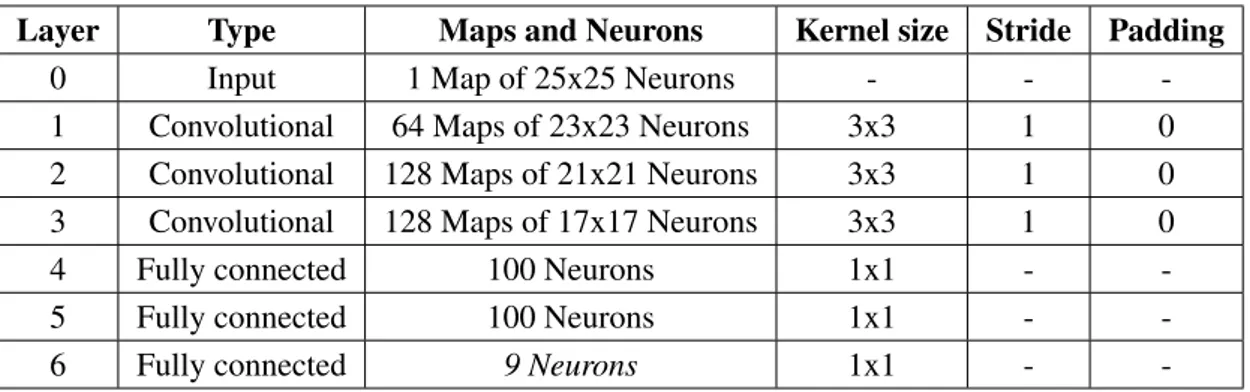
Melinscak et al. [48] performed retinal vessel segmentation using a CNN having max-pooling layers instead of subsampling or down-sampling. The layers of this CNN consist of a sequence of convolutional, max-pooling and fully connected layer. By using max-pooling it is possible to map input samples into output class probabilities using several hierarchical layers to classify extracted features [48] . This implementation is based on a CNN with 10 layers, whose architecture is presented on table3.4. The first layer is the input layer, then a bank of 2D filters is applied in each Table 3.4: Architecture of the implemented Convolutional Neural Network by Melinscak et al. [48].

Layer Type Maps and Neurons Kernel size Stride Padding

0 Input 1 Map of 65x65 Neurons - -

-1 Convolutional 48 Maps of 60x60 Neurons 6x6 1 0

2 Max-Pooling 48 Maps of 30x30 Neurons 2x2 1 0

3 Convolutional 48 Maps of 26x26 Neurons 5x5 2 2

4 Max-Pooling 48 Maps of 13x13 Neurons 2x2 1 0

5 Convolutional 48 Maps of 10x10 Neurons 4x4 2 0

6 Max-Pooling 48Maps of 5x5 Neurons 2x2 1 0

7 Convolutional 48Maps of 4x4 Neurons 2x2 2 0

8 Max-Pooling 48Maps of 2x2 Neurons 2x2 1 0

9 Fully connected 100 Neurons 1x1 -

-10 Fully connected 2 Neurons 1x1 -

-convolutional layer in order to obtain maps of features. Max-Pooling layers are fixed and take square blocks of Convolutional layers and reduce their output into a single feature. The selected feature is the most promising as Max-Pooling is carried out over the block. Following this, there are alternating steps of convolutional and Max-Pooling layers.

Finally, the last two layers are fully connected and they are used to further combine the previ-ous outputs, creating a 1D vector of features. The second fully connected layer has two neurons, one for each class, since the classification is binary (vessel or non-vessel). The final output is the probability of each pixel been being vessel [48].

This implementation was tested and trained on the DRIVE database and the most relevant results are presented on figure3.5 (in this particular case, the binary result of the segmentation

3.3 Supervised methods 21

wasn’t provided in the published paper, instead the presented image is result of the final softmax activation).

Figure 3.5: Best result of the best AUC score and Softmax activation obtained by Melinscak et al. [48].

Fu et al. [49] presented a segmentation method somehow similar to the work proposed by Melinscak et al. [48]. Contrasting with the methodology proposed by Melinscak et al. [48], Fu et al.[49] uses an image-to-image training system providing a multi-scale and multi-level visual response. This method uses a Fully Convolutional Neural Network to learn the discriminative features and generate a vessel probability map. Afterwards, a fully connected Conditional Random Field (CRF) accounts for global pixel correlation and produces a binary vessel segmentation result. Distinct from the method proposed by Melinscak et al. [48] that performs as a pixel-to-pixel classification, this proposed method treats the vessel segmentation as a contour detection problem. To tackle this, the Fully Convolutional Neural Network was built on top of a holistically-nested edge detection (HED) [50]. HED automatically learns rich hierarchical representations (guided by deep supervision on side responses) that are important to solve the challenging ambiguity in edge and object boundary detection. An example of a HED implementation is visible on the figure3.6 [50].

Considering this, Fu et al. [49] propose a four-stage implementation, in which each stage includes multiple convolutional and ReLu (Rectified Linear Unit) Layers. The side-output layers are connected to the last convolutional layer in each stage to deem the deep layer supervision [49]. The Conditional Random Fields are used to produce coarse maps at pixel-level segmentation and to suppress the lack of smoothness of the fully CNNs. The figure3.7 illustrates the presented approach.

One of the most interesting methods for retinal blood vessel segmentation using deep learning was proposed by Liskowski and Krawiec [51]. This method uses a deep neural network (CNN) trained on a large sample of examples pre-processed with global contrast normalization, and zero-phase whitening. Augmentation through geometric transformations and gamma correction was

22 State of the art

Figure 3.6: Network architecture for edge detection using HED [50].

Figure 3.7: Structure of the proposed method by Fu et al [49].

performed at training time [51].

The authors studied several variants of CNN architectures, such as including or not max-pool layers and the addition of structured prediction (where a network classifies multiple pixels simultaneously). This study uses three different databases (DRIVE, STARE and CHASE) to train, cross-train and test the all the architectures implemented. By doing so, this study is one of the most complete and detailed of all methodologies based on deep learning in the field of retinal blood vessel segmentation.

3.3 Supervised methods 23

pipeline). Afterwards, image processing is conducted, by means of global contrast normalization and zero-phase whitening. Even though deep learning architectures can learn from raw images, the authors experiments shown that such pre-processing increased the performance of the entire pipeline. For each training fundus image, 20 000 patches like this were generated at random, such that the training set has 400 000 patches in DRIVE and 380 000 in STARE [51]. The most relevant and noteworthy architectures studied by the authors are shown in table3.5.

Table 3.5: Two most relevant architectures proposed by Liskowski and Krawiec [51].

Implementation Layer Maps Kernel size Stride Padding

Plain Convolutional 64 4 x 4 1 0 Convolutional 64 3 x 3 1 1 Max-Pooling - 2 x 2 2 0 Convolutional 128 3 x 3 1 1 Convolutional 128 3 x 3 1 1 Max-Pooling - 2 x 2 2 0 Fully Connected 512 - - -Fully Connected 512 - - -Fully Connected 2 - - -No-POOL Convolutional 64 3 x 3 1 1 Convolutional 64 3 x 3 1 1 Convolutional 128 3 x 3 1 1 Convolutional 128 3 x 3 1 1 Fully Connected 512 - - -Fully Connected 512 - - -Fully Connected 2 - -

-The architectures presented on table3.5only differ in spatial pooling. The Max-Pooling pro-cess is performed over a 2 x 2 pixels window with a stride of 2 and is only used in the Plain implementation [51]. The No-POOL implementation does not use Max-pooling, since recent re-sults showed that networks which do not further down-sample the features might perform better when applied to small images [52].

Apart from these implementations, the authors considered four others, all using the Plain net-work architecture: GCN, ZCA, AUGMENTED and BALANCED. All are composed of a stack of convolutional layers that are followed by three Fully Connected layers (Table3.5). The main goal of these implementations was to analyse the performance of the Plain architecture when trained on data pre-processed by the methods previously described (Global Contrast Normalization, Zero-phase whitening and the image augmentations) and a on balanced data (with equal proportion of decision classes). An example of the data used in the training process is visible on the figures3.9 -3.10.

The different implementations were tested in both DRIVE and STARE databases with in-teresting results. Considering the overall experiment, the results outperform all of the previous algorithms published, relative to the most commons performance indicator, such as accuracy with average value superior to 0.97 on the STARE and area under the ROC curve averaging 0.99 on the

24 State of the art

Figure 3.8: Example of Train-ing patches after applying GCN transformation [51].

Figure 3.9: Example of Train-ing patches after applyTrain-ing ZCA whitening transformation [51].

Figure 3.10: Example of Train-ing patches usTrain-ing data augmen-tation [51].

STARE. The results also show that the proposed method is sensitive in the detection of fine vessel and fares well with pathological cases.

From the six implementations explained before, the best performance was achieved by the network trained on balanced data, obtaining the best-to-date results on both databases (considering the area under the ROC curve). The second best-performing architecture is the No-Pool. The two best performing architectures do not have pooling layers, what supports that down-sampling may be unworthy when small patches are being classified. Considering this, these layers may be discarded and by doing so, the dimensionality of the patches is kept across the entire network, allowing convolutional filters in successive layers to be applied at the same resolution.

Following this, Liskowski and Krawiec [51], using the two best architectures as base, also implemented structured prediction model. The addition of this model resulted on an improvement of the previously presented results increasing the AUC by 0.5% on DRIVE and 1.1% on STARE. In figure3.11, the best segmentations of this architecture in DRIVE (a) and STARE (b) databases are presented.

(a) (b)

Figure 3.11: Ground truth (left) and segmentation result (right) for two healthy subjects: (a) DRIVE and (b) STARE [51].

3.4 Summary and Comparison 25

3.4

Summary and Comparison

This chapter presented some of the most relevant approaches regarding retinal blood vessel seg-mentation. A summary of the performance of the described methods may be seen in table3.6. Such methods are grouped according to the learning technique and are presented in chronological order.

The fact that an extremely high percentage of the presented approaches used both the DRIVE and STARE databases allows a more simple, intuitive and incisive analyse and comparison of the performance indicators. However, in some of the methods, there are still a lack of consensus on which performance indicators should be considered to analyse and compare the overall perfor-mance of the algorithms.

Different methods based on different learning techniques have been proposed over time. The methods using unsupervised learning and based on morphological processing and vessel track-ing/tracing were the first to be proposed, studied and implemented. The results of these implemen-tations shown that the combination of different approaches delivers the best results considering the sensitivity and accuracy.

In recent years, the use of supervised leaning has grown exponentially. The implementation of machine learning based methodologies have shown an important improvement on specificity and accuracy, when compared to the unsupervised learning techniques.

Although machine learning methodologies have presented interesting results (as is example M.M Fraz et al. [3], Marin et al. [28] and Liskowski and Krawiec [51] ) the application of these are still conditioned to the existence of a ground truth. Nonetheless, when labelled data is available, as is the case of retinal fundus images, deep learning has been further improving the performance of computers in many daily tasks. In this particular task, deep learning has also outperformed other methods, as shown in the work of Liskowski and Krawiec [51].

26 State of the art

Table 3.6: Performance analysis of the methods presented in Chapter 3.

Performance indicators analysis

Learning Technique Methodology Algorithm Year Database Sensitivity Specificity Accuracy AUC 2o_{Human Observer - - -} DRIVE 0.7763 0.9723 0.9470

-STARE 0.8951 0.9384 0.9348

-Supervised Learning

Traditional Machine Learning

Staal et al. [40] 2004 DRIVE - - 0.9442 0.9520 STARE - - 0.9516 0.9614 Soares et al. [29] 2006 DRIVE - - 0.9466 0.9614 STARE - - 0.9480 0.9671 Ricci et al. [41] 2007 DRIVE - - 0.9563 0.9558 STARE - - 0.9584 0.9671 Marin et al. [42] 2011 DRIVE 0.7067 0.9801 0.9452 0.9588 STARE 0.6944 0.9819 0.9526 0.9769 M. M. Fraz et al. [43] 2012 DRIVE 0.7406 0.9807 0.9480 0.9747 STARE 0.7548 0.9763 0.9534 0.9768 CHASE_B1 0.7221 0.9711 0.9469 0.9712 Deep Learning

Wang et al. [44] 2014 DRIVE 0.8173 0.9733 0.9767 0.9475 STARE 0.8104 0.9791 0.9813 0.9751 Melinscak et al. [48] 2015 DRIVE - - 0.9466 0.9749

STARE - - - -Fu et al. [49] 2016 DRIVE 0.7294 - 0.9470 -STARE 0.7140 - 0.9545 -Liskowski and Krawiec [51] 2016 DRIVE 0.8149 0.9749 0.9530 0.9788

STARE 0.9075 0.9771 0.9700 0.9928

Unsupervised Learning

Unsupervised

Salem et al. [18] 2007 DRIVE 0.8215 0.9750 - -STARE - - - -Kande et al. [19] 2009 DRIVE - - 0.8911 0.9518

STARE - - 0.8976 0.9298 Villalobos-Castaldi et al.[20] 2010 DRIVE 0.9648 0.94803 0.9759 -STARE - - - -Match Filtering

Hoover et al. [22] 2000 DRIVE - - - -STARE 0.6751 0.9567 0.9267 -Zhang et al. [23] 2010 DRIVE 0.7120 0.9724 0.9382 -STARE 0.7177 0.9753 0.9484 -Morphological

Processing

Mendonça et al. [27] 2006 DRIVE 0.7344 0.9764 0.9452 -STARE 0.6996 0.9730 0.9440 -M.M Fraz et al. [35] 2010 DRIVE 0.7152 0.9769 0.9430 -STARE 0.7311 0.9680 0.9442 -Vessel

Tracking Delibasis et al. [34] 2010

DRIVE 0.7288 0.9505 0.9311 -STARE - - - -Multi-Scale approach Martinez-Perez et al.[36] 2007 DRIVE 0.7246 0.9655 0.9344 -STARE 0.7506 0.9569 0.9240

-Chapter 4

Methodology

Multiple approaches based on deep learning for the segmentation of retinal blood vessels have been implemented. Regarding those presented on chapter3, there are two different methodologies that use CNN’s in distinct manners in order to segment the vessels. These are the cornerstones of the work presented in this chapter.

The first methodology, used by Liskowski and Krawiec [51], Melinscak et al. [48], and Fu et al.[49] is an element-wise classification where the CNN is trained patch by patch and the output is the probability of the center pixel (or a block of center pixels in the case of structured prediction) being in a certain class (in this case a two class classification, as each pixel may be vessel or non vessel). These approaches use a large number M of small square N × N patches from raw RGB or pre-processed training set of images as input of the neural network. The network is trained and validated with said data and then tested with patches from the test dataset.

Other methodology of work is proposed by Wang et al. [44], where the authors use CNN as deep feature extractor. The main process is similar to the one previously presented, as it starts with a large number M of small square N × N patches from a pre-processed training dataset of images that are fed as input to the neural network. In contrast to the other methodology, the activations of a specific group of layers are used to train different machine learning classifiers (the authors use the Random forest classifier). The test images undergo the same process and the features extracted are fed into the classifier. To finalize the process an ensemble mechanism is used, from which the final classification of is obtained.

Regarding the first scenario, three different network architectures were implemented, in order to analyze how the architecture of the network as well as different parameters can influence the segmentation result. In what concerns the second framework, the approach proposed by Wang et al.[44] was implemented, and more complex ensemble mechanisms were tested. In addition, a Support Vector Machine classifier (SVM) in combination with feature selection algorithms was also implemented.

In the following section, the deviated solutions are described, starting with the data pre-processing mechanism which was used. Then, a detailed description of the implemented networks is provided. Lastly, the experiments regarding the work of Wang et al. [44], more precisely on