How well can models predict changes in species distributions? A 13-year-old otter model revisited

Hystrix, the Italian Journal of Mammalogy

Available online at:

http://www.italian-journal-of-mammalogy.it/article/view/11867/pdf doi:10.4404/hystrix-27.1-11867

Research Article

How well can models predict changes in species distributions? A 13-year-old otter model revisited

CIBIO/InBIO-Centro de Investigação em Biodiversidade e Recursos Genéticos, Universidade de Évora, 7004-516 Évora, Portugal

Keywords:

generalized linear models model performance model evaluation model extrapolation discrimination calibration Lutra lutra Article history: Received: 30 April 2016 Accepted: 24 June 2016 Acknowledgements

This work is part of JAG’s MSc dissertation, carried out within the Mas-ter’s in Conservation Biology of the University of Évora, under the super-vision of AMB and AM. AMB is supported by FCT and FEDER / COMPETE 2020 through contract IF/00266/2013, exploratory project CP1168/CT0001, and funds POCI-01-0145-FEDER-006821 to research unit UID/BIA/50027. We acknowledge the effort of over a hundred people who participated in the otter surveys that provided data for this study, and the sugges-tions of two anonymous reviewers who helped improve our manuscript.

Abstract

Species distribution and ecological niche models are increasingly used in biodiversity manage-ment and conservation. However, one thing that is important but rarely done is to follow up on the predictive performance of these models over time, to check if their predictions are fulfilled and maintain accuracy, or if they apply only to the set in which they were produced. In 2003, a distri-bution model of the Eurasian otter (Lutra lutra) in Spain was published, based on the results of a country-wide otter survey published in 1998. This model was built with logistic regression of otter presence-absence in UTM 10 km2_{cells on a diverse set of environmental, human and spatial} vari-ables, selected according to statistical criteria. Here we evaluate this model against the results of the most recent otter survey, carried out a decade later and after a significant expansion of the otter distribution area in this country. Despite the time elapsed and the evident changes in this species’ distribution, the model maintained a good predictive capacity, considering both discrimination and calibration measures. Otter distribution did not expand randomly or simply towards vicinity areas, but specifically towards the areas predicted as most favourable by the model based on data from 10 years before. This corroborates the utility of predictive distribution models, at least in the medium term and when they are made with robust methods and relevant predictor variables.

Introduction

The Eurasian otter (Lutra lutra) is a semi-aquatic carnivore whose worldwide distribution declined sharply between 1950 and 1970, largely due to direct persecution and habitat destruction. This trend was reversed by local conservation efforts towards the end of that cen-tury (Ruiz-Olmo and Delibes, 1998; Trindade et al., 1998). The spe-cies is still recovering nowadays, especially in Western Europe, but is considered Near Threatened globally, based mainly on sensitivity to changes and on ongoing declines in parts of its distribution range (IUCN, 2015).

Being able to predict the evolution of the geographical range of a species may be crucial when there is a need to design conservation or management plans that stay effective (e.g., Carone et al., 2014). Al-though it is difficult to collect variables that include all the ecological restrictions and species interactions that shape the geographical range of a species, it is often possible to develop accurate models (Liu et al., 2011). When creating a species distribution model (SDM), besides relevant information on environmental variables related to the occur-rence of the target species, we need a representative set of presence (and preferably also absence) records to use as “training data” for the model (Fielding and Bell, 1997). After building the model, we need to evaluate its predictive ability. It is generally recommended that this evaluation is based on “testing data” not used in the development of the model (Fielding and Bell, 1997).

One way of assessing whether a model has correctly captured the species-environment relationships, and is thus actually capable of pre-dicting species distributions, can be to confront the model with data

∗

Corresponding author

Email address: barbosa@uevora.pt (A. Márcia Barbosa)

from the “future” — i.e., data that did not exist at the time the model was built, and that ideally reflect actual changes in the target species’ distri-bution. If the model still performs well after such unforeseen changes, then we can reasonably assume that it has captured the relevant drivers of species occurrence, and is thus reliable for use in management and conservation planning.

The Eurasian otter (Lutra lutra) provides an excellent case study for such an analysis, for several reasons. First, it is a well-known species, whose ecological behaviour and habitat preferences have been widely studied, and which has been the subject of thorough nation-wide dis-tribution surveys (e.g., Delibes, 1990; Ruiz-Olmo and Delibes, 1998). Second, its distribution in Spain has been modelled previously, and the results were then published and extrapolated to a finer resolution (Barbosa et al., 2003). Third, a more recent otter survey in this coun-try (López-Martín and Jiménez, 2008) reflected a substantial expansion regarding the occurrence area that was used for training the previously published model. This provides an excellent opportunity to assess if this expansion is happening towards the most favourable places pre-dicted by the model based on data from ten years earlier, and if this SDM can thus keep a good performance on tracking the otter distribu-tion.

In this paper we test an otter distribution model against data from the model’s “future”, i.e., from ten years after the survey whose data were used for model training. We quantify the changes in otter distribution and assess if those changes were in agreement with the model predic-tions, rather than happening simply around the vicinity of the previous presence areas. We thus assess the utility of SDMs for informing man-agement and conservation plans.

Hystrix, the Italian Journal of Mammalogy ISSN 1825-5272 5th August 2016

Figure 1 – (a) Presence/absence of otter records on UTM 10×10 km cells, after the

pen-ultimate Spanish otter survey (Ruiz-Olmo and Delibes, 1998); (b) presence/absence points georeferenced from the last otter survey (López-Martín and Jiménez, 2008); (c) presence probability predicted for these points by the model of Barbosa et al. (2003), built on the data in a).

Methods

Model predictions were those obtained by Barbosa et al. (2003). The model consisted of a logistic regression (generalized linear model with binomial error distribution and logit link) of the presence/absence of otter records on UTM 10×10 km cells of mainland Spain (Fig. 1a). These records resulted from a previous nation-wide otter survey (Ruiz-Olmo and Delibes, 1998). The predictors were a set of environmental, human and spatial variables (Tab. 1), which were included in the model with a forward conditional stepwise selection procedure (Barbosa et al., 2003).

In order to assess the predictive power of the model, we used the results of the most recent otter survey in Spain (López-Martín and Jiménez, 2008) as test data. We gathered all maps with the results from each mainland Spanish province, including both presence and ab-sence points, digitized and georeferenced them in a single points layer. We used an open-source geographical information system, QGIS 2.4 (QGIS Development Team,QGIS, 2014), and its Georeferencer plugin.

Table 1 – Predictor variables used for building the otter distribution model evaluated here,

and the signs of those that were finally included in the model. For more details see Barbosa et al. (2003).

Type Variable Sign

Environmental Morning air humidity in January

Morning air humidity in July + Annual air humidity range

Potential evapotranspiration

Actual evapotranspiration +

Annual insolation

Annual solar radiation +

Mean January temperature –

Mean July temperature +

Annual mean temperature –

Annual temperature range Annual number of frost days Annual number of rain days

Annual mean precipitation +

Maximum precipitation in 24 hours Relative maximum precipitation Pluviometric irregularity Annual run-off

Soil permeability –

Mean altitude –

Human Distance to a motorway +

Distance to a town >100000 inhabitants + Distance to a town >500000 inhabitants +

Spatial Mean latitude +

Mean longitude –

We overlaid this map of recently surveyed presence and absence points to the UTM 10×10 km grid that was used for model training (Barbosa et al., 2003), to extract the sampled presences and absences at the same spatial resolution at which the model was built. We also ex-tracted the predicted probability value for each sampling point, using the model predictions downscaled to 1 km2 pixels (Fig. 7 of Barbosa et al., 2003), using the Point Sampling Tool plugin of QGIS.

Statistical analyses

To perform the statistical analyses, we used the open-source software R 3.1 (R Core Team, 2014). We first assessed the changes in otter distri-bution from the previous Spanish otter survey (Ruiz-Olmo and Delibes, 1998), used as model training data, to the latest survey (López-Martín and Jiménez, 2008), used here as model testing data. We quantified the gained, maintained and lost presences between both surveys on UTM 10×10 km grid cells.

We then confronted the model predictions with the test data derived from the latest survey. We used a suite of model evaluation measures implemented in the modEvA R package (Barbosa et al., 2013), which assess two different components of model performance: discrimina-tion (i.e., the ability of the model to distinguish presence from absence localities); and calibration or reliability (i.e., the deviations of continu-ous model predictions from actual observations). Although the latter component is usually neglected, it is just as important in the evaluation of species distribution models (Pearce and Ferrier, 2000; Wintle et al., 2005; Jiménez-Valverde et al., 2013).

To investigate whether the changes in otter distribution occurred simply around the vicinity of previously occupied areas rather than specifically according to the combination of predictor variables in the model, we also did a spatial interpolation model based on simple in-verse distance to presence (Takahashi et al., 2014), using the distPres function of the fuzzySim R package (Barbosa, 2015a). We then ap-plied the set of model evaluation measures to this spatial interpolation model as well.

To evaluate the predictions of the model when extrapolated to 1 km2 cells, we compared mean predicted probability among presence and

ab-sence points. For this we used box plot notches (Chambers et al., 1983) and the non-parametric signed rank test of Mann-Whitney-Wilcoxon (Wilcoxon, 1945).

Results

Observed changes in otter distribution

We georeferenced 4966 points surveyed in mainland Spain in the latest nation-wide otter survey (López-Martín and Jiménez, 2008). Among these, 3255 points (65.5%) were classified as presences and 1711 points (34.5%) were classified as absences (Fig. 1b).

When gridded to the 10×10 km UTM cells that were originally used for building the model (Barbosa et al., 2003), these recently surveyed points yielded 2625 presence cells and 2542 absence cells (i.e. cells with no presence records). When compared to the data from the

previ-ous otter survey (Ruiz-Olmo and Delibes, 1998), on which the model was built, there were 1384 new presences, representing a 90.6% in-crease; 1241 (81.3%) maintained presences; and 286 (18.7%) lost pres-ences, i.e., UTM cells with presence records in the 1998 survey and no presence records in the latest survey.

Evaluation of the model on 10 km2 _{grid cells}

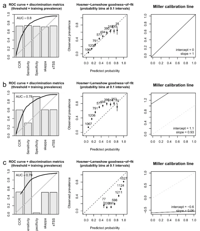
When applied to the test data from the latest otter survey, the model trained on the previous survey achieved generally similar performance measures. There was a visible decrease in sensitivity (i.e., the ability to detect presences) from the training to the test data (Fig. 2), indicating that the model did not predict such a substantial increase in the otter oc-currence area. However, test presences did have higher predicted prob-abilities than test absences, as the area under the curve (AUC) of the receiver operating characteristic (ROC) of the model applied to the test

Figure 2 – Model evaluation measures obtained for the otter distribution model of Barbosa et al. (2003) when confronted with the training data (a) and with more recent test data (b),

and the same measures for a distance interpolation of the training data compared to the test data (c). CCR: overall correct classification rate; TSS: true skill statistic. TSS and kappa were standardized (s) to vary between 0 and 1 and thus be directly comparable to the other measures (Barbosa, 2015b).

Table 2 – Proportion of explained deviance (D2) and different pseudo-R2measures ob-tained for the otter distribution model of Barbosa et al. (2003) when compared to the training data (Ruiz-Olmo and Delibes, 1998) and to more recent test data (López-Martín and Jiménez, 2008); and the same measures for a distance interpolation model applied to the test data.

Model vs. Model vs. Distance vs. Evaluation

training data test data test data

D2 0.19 0.18 0.13 R2 Cox-Snell 0.21 0.22 0.16 R2 Nagelkerke 0.30 0.29 0.21 R2 McFadden 0.19 0.18 0.13 R2 Tjur 0.22 0.19 0.13 R2 Pearson 0.19 0.21 0.24

data was not significantly different from the AUC of the model on the training data (Fig. 2; DeLong’s test for two ROC curves, calculated with the pROC package (Robin et al., 2011), p>0.05). The distance interpol-ation of training data had a slightly higher AUC than the model when classifying the test data, but the results of other discrimination meas-ures (including e.g. the widely used True Skill Statistic and Cohen’s kappa, which controls for chance effects in the agreement between pre-dictions and observations) were generally worse than those obtained by the Barbosa et al. (2003) model on the test data (Fig. 2).

The proportion of variation accounted for by the model also did not vary visibly among training and test data, with explained devi-ance and most pseudo-R2measures remaining essentially the same in both datasets. Conversely, the distance interpolation yielded visibly smaller values for nearly all these metrics (Tab. 2). Regarding calibra-tion, the model underestimated occurrence frequencies in the test data (again, not predicting such an extensive increase in the otter distribu-tion area), according to both the Hosmer-Lemeshow goodness-of-fit and the Miller calibration plots (Fig. 2). However, the Miller calibra-tion line was practically parallel to the diagonal, with a slope of nearly 1 — i.e., predictions were consistently below observations (bias), but varied proportionally to them (no spread). Conversely, the distance in-terpolation overestimated otter occurrence in the test data and not in a consistent or directly proportional way, as both Miller intercept and slope were far from the ideal values of 0 and 1, respectively (Fig. 2).

Evaluation of the model when downscaled to 1 km2 pixels

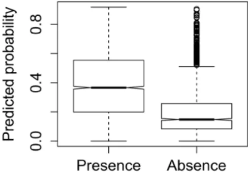
The values of predicted probability provided by the model downscaled to 1 km2resolution (Barbosa et al., 2003) were visibly higher for test presence than for test absence points (Fig. 3). The notches (“waists”) of their box plots did not overlap, thus providing strong evidence that the two medians differ (Chambers et al., 1983, p. 62). The Wilcoxon rank-sum test also showed a significant difference between the mean prob-ability values predicted for presence and absence points (W =1315001, p<2.2×10-16).

Figure 3 – Box plot of the otter presence probability values predicted by the model of

Barbosa et al. (2003) for the test presence and absence points obtained from the latest otter survey (López-Martín and Jiménez, 2008).

Discussion

Species distribution models are now routinely used in ecology and biogeography (see e.g. Jiménez-Valverde and Lobo, 2007 for a brief review). A trustworthy evaluation of their predictive capacity is cru-cial, especially if models are to be taken into account when designing conservation and management plans. Such evaluation should be made not only on data contemporaneous to the model, but also on data that the modellers had no way of accessing when the model was built. Here we evaluated an otter distribution model using test data from several years after the model was published, and which included visible changes in the distribution of the modelled species.

As is usual with widespread species, measures of model discrimin-ation (i.e., the ability to distinguish presence sites from absence sites) were already not very high for the original model when evaluated on the training data (Fig. 2a), and they remained essentially similar in the evaluation on the test data. Sensitivity was the clear exception, with a significant amount of new presences falling in areas predicted as having relatively low presence probability (Fig. 2b). However, this mismatch was only quantitative rather than qualitative: these areas still had gen-erally higher probability than those where the otter remained absent, as was evidenced by an AUC not significantly lower than that obtained for the model on the training data (Fig. 2a). This means that not many places outside the training occurrence areas had high probability of being occupied, although they were; but, within those areas, the otter expanded to the ones with still relatively high probability.

The recently occupied areas were necessarily in the vicinity of the previously occupied ones, so the model based on simple distance inter-polation also obtained a relatively high AUC. However, although the distance interpolation model did capture nearly all the new presences, it had very low specificity, i.e. was largely unsuccessful at predicting otter absences, unlike the distribution model of Barbosa et al. (2003), which did achieve a high prediction success on absences. Accuracy measures that take into account overall classification success correct-ing for chance effects, such as Cohen’s kappa, also detected a visibly better performance of model predictions against the distance interpol-ation (Fig. 2b,c).

Measures of model calibration and explained deviance provided even stronger support for the superior reliability of the generalised linear model over simple distance interpolation. While the model did under-estimate otter occurrence, its nearly parallel calibration line showed that it captured the species-environment relationships almost perfectly, unlike the distance interpolation (Fig. 2b,c). Hence, the otter expan-sion documented in López-Martín and Jiménez (2008) occurred not randomly, nor simply towards the neighbourhood of the occurrences detected in the previous otter survey, but rather precisely towards the areas predicted with higher probabilities by the model published sev-eral years before (Barbosa et al., 2003).

Resolution scale is important too, as coarse-scale data can some-times disguise fine-scale discontinuities (e.g., Sales-Luís et al., 2012). The analysed model was previously extrapolated to predict otter distri-bution at a 100-times finer resolution scale (Barbosa et al., 2003), and it was evaluated at this scale using point data from the previous otter survey (Barbosa et al., 2010). Here we evaluated the model also on point data from the latest survey. The comparison between point re-cords and downscaled model predictions kept in line with the previous results, with presence points located in pixels predicted with clearly higher probability values than absence points. There were, however, several outliers, with a set of absence points in areas predicted as hav-ing high probabilities of occurrence (Fig. 3), and a maximum predicted value for absences (0.958) very close to the maximum obtained for presences (0.964). There are thus few but visible areas of disagree-ment, where the model predicts highly favourable conditions for the otter to be present, but where no presence signs were detected. Field-ing and Bell (1997) suggest that such cases indicate ecological interfer-ences that the model could not predict — for example, dispersal barri-ers or biotic interactions such as competition or lack of prey. Another important justification might be the alteration or destruction of otter habitat, possibly associated to changes in the human variables over the

last decade (e.g., Pedroso et al., 2014). Further research should focus on understanding what kinds of obstacles are inhibiting the otter from completely occupying its potential range.

Conversely, there were generally low predicted values in the north-east (Fig. 1c), where the otter is known to be currently expanding. The analysed model was based on data from the beginning of the otter recov-ery in Spain (Ruiz-Olmo and Delibes, 1998), when this species was still mostly distributed in the western half of this country (Fig. 1a). The otter had previously gone virtually extinct in eastern Spain (Delibes, 1990) and has since recovered increasingly in this region (López-Martín and Jiménez, 2008), as has happened in other parts of Europe (Romanowski et al., 2013). This probably had some weight in the results: the model was built for the complete country at an initial stage of the eastern re-covery, so it gathered more occurrence information from the most typ-ical or common otter habitats in western Spain. Typtyp-ical habitats of the eastern Spanish otters, which can be different from those in the west, were thus less analysed by the model.

In addition, the model included two spatial variables, latitude and longitude (Tab. 1), reflecting spatial trends that are not explained by the available environmental and human variables (Barbosa et al., 2003). These variables can account for spatially contagious biotic processes such as reproduction, migration, and mortality (Legendre, 1993), and they may have limited the probability predictions in eastern Spain, where the recent otter expansion was aided, at least in part, by a re-introduction programme (Fernández-Morán et al., 2002).The existence of both favourable and unfavourable areas within the current otter range could also suggest a metapopulation structure or the occurrence of source-sink dynamics, with expanding populations occupying subop-timal habitats when opsubop-timal ones have reached their carrying capacity (Pulliam, 1988; Muñoz et al., 2005; John et al., 2010). Otters could also be increasing their habitat tolerances in formerly inadequate areas, as has already been observed in eastern Europe (Romanowski et al., 2013).

All in all, although the analysed model was developed with otter dis-tribution data from the last century, it showed considerable accuracy in predicting the results of a subsequent otter survey carried out ten years later, and in distinguishing the otter expansion areas from those where the species still does not naturally occur. This provides support for the utility of SDMs in conservation and management planning, at least when these models are built with robust and extrapolable meth-ods, as generalised linear models have widely proven to be (Ennis et al., 1998; Elith, 2000; Wintle et al., 2005; Farfán et al., 2008; Barbosa et al., 2009); with a diverse enough set of variables to capture the rel-evant correlates of the species’ distribution (Tab. 1); and with strong statistical methods to select among such variables (see Barbosa et al., 2003). Evaluating models against data from their future is a reliable and necessary way to assess their actual predictive power.

References

Barbosa A.M., Real R., Muñoz A.-R., Brown J.A., 2013. New measures for assessing model equilibrium and prediction mismatch in species distribution models. Divers. Distrib. 19: 1333–1338.

Barbosa A.M., Real R., Olivero J., Vargas J.M., 2003. Otter (Lutra lutra) distribution mod-elling at two resolution scales suited to conservation planning in the Iberian Peninsula. Biol. Conserv. 114: 377–387.

Barbosa A.M., Real R., Vargas J.M., 2009. Transferability of environmental favourability models in geographic space: the case of the Iberian desman (Galemys pyrenaicus) in Portugal and Spain. Ecol. Modell. 220: 747–754.

Barbosa A.M., Real R., Vargas J.M., 2010. Use of coarse-resolution models of species’ distributions to guide local conservation inferences. Conserv. Biol. 24: 1378–87. Barbosa A.M., 2015a. fuzzySim: applying fuzzy logic to binary similarity indices in

eco-logy. Methods Ecol. Evol. 6: 853–858.

Barbosa A.M., 2015b. Re-scaling of model evaluation measures to allow direct comparison of their values. J. Br. Ideas.

Carone M.T., Guisan A., Cianfrani C., Simoniello T., Loy A., Carranza M.L., 2014. A multi-temporal approach to model endangered species distribution in Europe. The case of the Eurasian otter in Italy. Ecol. Modell. 274: 21–28.

Chambers J.M., Cleveland W.S., Kleiner B., Tukey P.A., 1983. Graphical Methods for Data Analysis. Wadsworth and Brooks/Cole.

Delibes M., 1990. La Nutria (Lutra lutra) en España. Madrid: Ministerio de Agricultura, Pesca y Alimentación / ICONA.

Elith J., 2000. Quantitative Methods for Modeling Species Habitat: Comparative Perform-ance and an Application to Australian Plants. Quantitative Methods for Conservation Biology. New York: Springer-Verlag. p. 39–58.

Ennis M., Hinton G., Naylor D., Revow M., Tibshirani R., 1998. A comparison of statistical learning methods on the GUSTO database. Stat. Med. 17: 2501–2508.

Farfán M.A., Vargas J.M., Guerrero J.C., Barbosa A.M., Duarte J., Real R., 2008. Distri-bution modelling of wild rabbit hunting yields in its original area (S Iberian Peninsula). Ital. J. Zool. 75: 161–172.

Fernández-Morán J., Saavedra D., Manteca-Vilanova X., 2002. Reintroduction of the Euras-ian otter (Lutra lutra) in northeastern Spain: trapping, handling, and medical manage-ment. J. Zoo Wildl. Med. 33: 222–227.

Fielding A.H., Bell J.F., 1997. A review of methods for the assessment of prediction errors in conservation presence/absence models. Environ. Conserv. 24: 38–49.

IUCN, 2015. The IUCN List of Threatened Species, version 2015.1. Available from http: //www.iucnredlist.org.

Jiménez-Valverde A., Acevedo P., Barbosa A.M., Lobo J.M., Real R., 2013. Discrimina-tion capacity in species distribuDiscrimina-tion models depends on the representativeness of the environmental domain. Glob. Ecol. Biogeogr. 22: 508–516.

Jiménez-Valverde A., Lobo J.M., 2007. Threshold criteria for conversion of probability of species presence to either–or presence–absence. Acta Oecologica. 31: 361–369. John F., Baker S., Kostkan V., 2010. Habitat selection of an expanding beaver (Castor fiber)

population in central and upper Morava River basin. Eur. J. Wildl. Res. 56: 663–671. Legendre P., 1993. Spatial autocorrelation: trouble or new paradigm? Ecology. 74: 1659–

1673.

Liu C., White M., Newell G., 2011. Measuring and comparing the accuracy of species distribution models with presence-absence data. Ecography. 34: 232–243.

López-Martín J.M., Jiménez J. , 2008. La nutria en España. Veinte años de seguimiento de un mamífero amenazado. Málaga: SECEM.

Muñoz A.R., Real R., Barbosa A.M., Vargas J.M., 2005. Modelling the distribution of Bonelli’s eagle in Spain: implications for conservation planning. Divers. Distrib. 11: 477–486.

Pearce J., Ferrier S., 2000. Evaluating the Predictive Performance of Habitat Models De-veloped using Logistic Regression. Ecol. Modell. 133: 225–245.

Pedroso N.M., Marques T.A., Santos-Reis M., 2014. The response of otters to envir-onmental changes imposed by the construction of large dams. Aquat. Conserv. Mar. Freshw. Ecosyst. 24: 66–80.

Pulliam H.R., 1988. Sources, sinks, and population regulation. Am. Nat. 132: 652–661. QGIS Development Team, 2014. QGIS Geographic Information System.

R Core Team, 2014. R: A language and environment for statistical computing.

Robin X., Turck N., Hainard A., Tiberti N., Lisacek F., Sanchez J.-C., Müller M., 2011. pROC: an open-source package for R and S+ to analyze and compare ROC curves. BMC Bioinformatics. 12: 77.

Romanowski J., Brzeziński M., Zmihorski M., 2013. Habitat correlates of the Eurasian otter Lutra lutra recolonizing Central Poland. Acta Theriol. 58: 149–155.

Ruiz-Olmo J., Delibes M., 1998. La nutria en España ante el horizonte del año 2000. Málaga: Sociedad Española para la Conservación y Estudio de los Mamíferos. Sales-Luís T., Bissonette J.A., Santos-Reis M., 2012. Conservation of Mediterranean otters:

the influence of map scale resolution. Biodivers. Conserv. 21: 2061–2073.

Takahashi M.K., Eastman J.M., Griffin D.A., Baumsteiger J., Parris M.J., Storfer A., 2014. A stable niche assumption-free test of ecological divergence. Mol. Phylogenet. Evol. 76: 211–226.

Trindade A., Farinha N., Florêncio E., 1998. A distribuição da lontra Lutra lutra em Por-tugal – situação em 1995. Lisboa: ICN.

Wilcoxon F., 1945. Individual comparisons by ranking methods. Biometrics Bull. 1: 80–83. Wintle B.A., Elith J., Potts J.M., 2005. Fauna habitat modelling and mapping: A review and case study in the Lower Hunter Central Coast region of NSW. Austral Ecol. 30: 719–738.