Pesqui. Oper. vol.36 número2

doi: 10.1590/0101-7438.2016.036.02.0345

AN ALTERNATIVE REPARAMETRIZATION FOR THE WEIGHTED LINDLEY DISTRIBUTION

Josmar Mazucheli

_{, Em´ılio Augusto Coelho-Barros}

and Jorge Alberto Achcar

Received February 19, 2015 / Accepted June 4, 2016

ABSTRACT.Recently, [12] introduced a generalization of a one parameter Lindley distribution and named it as a weighted Lindley distribution. Considering this new introduced weighted Lindley distribution, we propose a reparametrization on the shape parameter leading it to be orthogonal to the other shape parameter. In this alternative parametrization, we get a direct interpretation for this transformed parameter which is the mean survival time. For illustrative purposes, the weighted Lindley distribution on the new parametrization is applied on two real data sets. The one parameter Lindley distribution and its generalized form are fitted for the considered data sets.

Keywords: generalized Lindley distribution, Lindley distribution, orthogonal parameters, survival analysis, weighted Lindley distribution.

1 INTRODUCTION

A non negative random variable T follows the two-parameter weighted Lindley distribution, [12], with shape parametersµ >0 andβ >0 if its probability density function is given by:

f (t |µ, β)= µ β+1

(µ+β) Ŵ (β)t

β−1_(1+t)e−µt_{, (1)}

wheret > 0 andŴ (β) = ₀∞tβ−1e−tdt is the gamma function. From(1), the corresponding survival and hazard functions, are given, respectively, by:

S(t|µ, β)= (µ+β) Ŵ (β, µt)+(µt) β_e−µt

(µ+β) Ŵ (β) , (2)

*Corresponding author.

1Universidade Estadual de Maring´a, Departamento de Estat´ıstica, Maring´a, PR, Brasil. E-mail: jmazucheli@gmail.com 2Universidade Tecnol´ogica Federal do Paran´a, Departamento Acadˆemico de Matem´atica, Corn´elio Proc´opio, PR, Brasil. E-mail: eabarros@utfpr.edu.br

and

h(t|µ, β)= µ

β+1_tβ−1_(1+t)e−µt

(µ+β) Ŵ (β, µt)+(µt)βe−µt, (3)

whereŴ (a,b),a >0 andb≥0, is the upper incomplete gamma function (see, [29]), defined as

∞

b ta−1e−tdt.

In (1), taking the shape parameterβ =1 we have the one parameter Lindley distribution as a special case. The one parameter Lindley distribution was introduced by Lindley (see, Lindley 1958 and 1965) as a new distribution useful to analyze lifetime data, especially in applications modeling stress-strength reliability. [13] studied the properties of the one parameter Lindley distribution under a careful mathematical approach. These authors also showed, in a numeri-cal example, that the Lindley distribution usually gives better fit for the data when compared to the standard Exponential distribution. A generalized Lindley distribution, which includes as special cases the Exponential and Gamma distributions was introduced by [36]. Ghitany and Al-Mutari (2008) considered a size-biased Poisson-Lindley distribution and [31] introduced the Poisson-Lindley distribution to model count data. Some properties of the Poisson-Lindley distri-bution, its derived distributions and some mixtures of this distribution were studied by [5, 6, 24]. A zero-truncated Lindley was considered in [10]. A study on the inflated Poisson-Lindley distribution was presented in [7] and the Negative Binomial-Poisson-Lindley distribution was introduced in [37]. The one parameter Lindley distribution in the competing risks scenario was considered in [26].

Since the standard one parameter Lindley distribution does not provide enough flexibility to analyze different types of lifetime data, the two-parameter weighted Lindley distribution could be a good alternative in the analysis of lifetime data. A nice feature of the two-parameter weighted Lindley distribution is that its hazard function has a bathtub form for 0 < β < 1 and it is increasing forβ≥1, for allµ >0.

It is important to point out, that in the last years, several distributions have been introduced in the literature to model bathtub hazard functions but in general these distributions have three or more parameters usually depending on numerical methods to find the maximum likelihood estimates which could be, in general, not very accurate. In this case good reparametrizations with less parameters could be very useful in applications. A comprehensive review of the existing know distributions that exhibit bathtub shape is provided in [30, 17, 3, 28]. In addition to the weighted Lindley distribution, that can be used to model bathtub-shaped failure rate, we also could consider as alternatives, four other two-parameter distributions introduced in the literature [18, 8, 15, 35] with this behavior.

matrix is diagonal. Other advantage of orthogonal parameters is related to the conditional like-lihood approach (for further details see, Cox & Reid, 1987; Lancaster, 2002; Louzada–Neto & Pardo–Fernandez, 2001; Louzada & Cavali, 2014).

The paper is organized as follows. In Section 2 the likelihood function for the two-parameter weighted Lindley distribution is formulated where we also present the proposed orthogonal reparametrization. Two examples considering real data sets are provided in Section 3 where its observed that the weighted Lindley distribution gives better fit for the data when compared to the one-parameter Lindley distribution and the generalized Lindley distribution. Some conclusions are presented in Section 4.

2 THE LIKELIHOOD FUNCTION

Lett=(t1, . . . ,tn)be a realization of the random sampleT=(T1, . . . ,Tn), whereT1, . . . ,Tn

are i.i.d. (identically independent distribution) random variables according to a two-parameter Lindley distribution, with shape parametersµ >0 andβ >0. From(1)the likelihood function can be written as:

L(µ, β|t)=

µβ+1 (µ+β) Ŵ (β)

n e−µT0

n

i=1

t_iβ−1(1+ti) , (4)

whereT0 = ni=1ti andŴ (β) =

∞

0 yβ−1e−yd yis the gamma function. From(4), the log-likelihood function forµandβ,l(µ, β|t), is given by:

l(α, β |t)=n(β+1)log(µ)−log(µ+β)−logŴ (β)−µT0+(β−1)T1+T2, (5)

whereT1=

n

i=1log(ti)andT2=

n

i=1log(1+ti).

Differentiating(5)with respect toµandβand setting the results equal to zero we have:

∂

∂µl(µ, β|t) = n β+1

µ −

1

(µ+β)

−T0=0, (6)

∂

∂βl(µ, β|t) = n log(µ)−

1

(µ+β)−ψ (β)

+T1=0, (7)

whereψ (β) = _dd_βlogŴ (β)is the digamma function. The maximum likelihood estimates, µˆ

andβˆ, for µ andβ, respectively, are obtained by solving equations(6)and(7)inµ andβ, respectively.

From(6), the maximum likelihood estimate forµis obtained as a function ofβ,µ (β)ˆ , given by:

ˆ

µ (β)=β (n−T0)+

β2_(n+T

0)2+4nβT0 2T0

. (8)

the maximum likelihood estimator forβ. With the obtained maximum likelihood estimator forβ

get the maximum likelihood estimator forµusing equation(8).

Based on a single observation, the observed information matrix,I(µ, β), is given by:

I(µ, β)=

⎛ ⎜ ⎜ ⎝

β+1

µ2 − 1

(µ+β)2 −

1

µ+

1

(µ+β)2

−_µ1 + 1 (µ+β)2

ψ′(β)− 1 (µ+β)2

⎞ ⎟ ⎟

⎠, (9)

whereψ′(β) = _dd2

β2 logŴ (β), and the terms in the(2×2)observed Fisher information matrix

(9)are obtained from the second derivatives given by,

I11(µ, β)= −

∂2

∂µ2l(µ, β|t) , I22(µ, β)= −

∂2

∂β2l(µ, β|t) and

I12(µ, β)= −

∂2

∂µ∂βl(µ, β|t) .

The maximum likelihood estimates forµandβ have asymptotic bivariate normal distribution with mean(µ, β)and variance-covariance matrix given by the inverse of the Fisher Information matrix(9)locally at the maximum likelihood estimatesµˆ andβˆ. Since the data is independent, the information matrix(9)is equal to the expected information matrix.

In this paper we propose to reparametrize the two-parameter weighted Lindley distribution such that(µ, β)is transformed to(θ , β), where:

θ=g(µ, β)= β (µ+β+1)

µ (µ+β) (10)

whereθ >0 is the mean of the weighted Lindley distribution with parametersµandβand

g−1(θ )=µ= β (1−θ )+

β2_(θ−1)2_{+4θ β (β+1)}

2θ .

Using the construction method of orthogonality parameters, proposed in [9], and from(9)we observe thatµis obtained as solution of the following orthogonality differential equation:

I11(µ,β)

β+1

µ2 − 1

(µ+β)2

∂µ ∂β − 1 µ + 1

(µ+β)2

I12(µ,β)

=0 (11)

In this new parametrization we have that the maximum likelihood estimate for θ is given by

ˆ

θ = n−1n_i=1ti andCov

ˆ θ ,βˆ

3 APPLICATIONS

In this section we fit the two-parameter weighted Lindley distribution (WL) to two real data sets. For comparative purposes we also have considered two alternative models: (L): the one parameter Lindley distribution,f (t |µ)=_µµ₊2₁(1+t)e−µt, and (GL): the generalized Lindley

distribution,f (t|µ, β, γ )=_{(µ+γ )Ŵ(β}µβ+1₊₁₎(β+γt)tβ−1e−µt, [36].

The first data set was reported by [4], and employed by [14] among others, represents the survival times (in days) of 72 guinea pigs infected with virulent tubercle bacilli, regimen 4.3. The regimen number is the common log of the number of bacillary units in 0.5 ml of challenge solution. The second data set was extracted from [33], see also [25], representing hours to failure of 59 test conductors of 400-micrometer length. All specimens ran to failure at a certain high temperature and current density. The 59 specimens were all tested under the same temperature and current density.

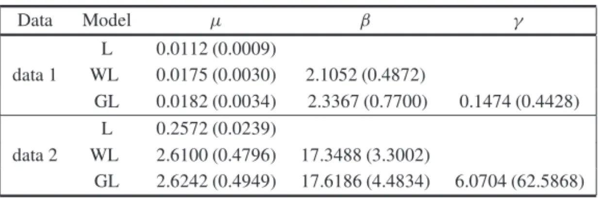
Table 1 list for the two data sets and models L, WL and GL the maximum likelihood estimates and their standard errors. For comparative purposes the estimates are also presented in the orig-inal parameterization and were obtained usingSAS/NLMIXED procedure, [32], by applying the Newton-Raphson algorithm. For the WL model, in the orthogonal parameterization, we have

θ = t = 176.82 (data set 1) andθ = t = 6.98 (data set 2). The standard errors are given, respectively, by 11.86 and 0.21.

Table 1 – Maximum likelihood (standard error) estimates for Lindley (L), weighted Lindley (WL) and generalized Lindley (GL) distribution.

Data Model µ β γ

L 0.0112 (0.0009)

data 1 WL 0.0175 (0.0030) 2.1052 (0.4872)

GL 0.0182 (0.0034) 2.3367 (0.7700) 0.1474 (0.4428) L 0.2572 (0.0239)

data 2 WL 2.6100 (0.4796) 17.3488 (3.3002)

GL 2.6242 (0.4949) 17.6186 (4.4834) 6.0704 (62.5868)

In Table 2 are listed standard model selection measures: −2×log-likelihood, AI C (Akaike’s Information Criterion, [1]) and B I C (Schwarz’s Bayesian Information Criterion, [34]). From the values of these statistics we conclude that the two parameter Lindley distribution provides a better fit for the data sets when compared to the two alternative models. For the WL model the obtained estimates forθare respectively given by: 176.82 (data set 1) and 6.98 (data set 2). The standard errors are given by, 11.86 and 0.21, respectively.

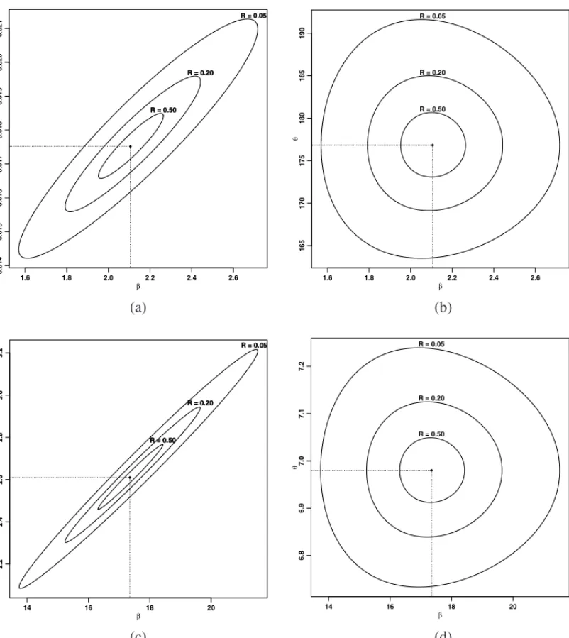
For illustrative purposes, we present in Figure 1 the 50%, 90% and 95% likelihood contour plots in the original and the proposed orthogonal parametrization. In contrast to panels(b,data set 1)

and(d,data set 2), the orientation of the contours in panels (a,data set 1)and(c,data set 2)

Table 2–Model selection measures.

Data Model -2 log-like AIC BIC

L 858.6 860.6 862.8

Data 1 WL 851.5 855.5 860.1

GL 851.3 857.3 864.2

L 316.7 318.7 320.8

Data 2 WL 223.6 227.6 231.8

GL 223.6 229.6 235.9

axes of the elliptical contours are parallel to the coordinate axes, and for this reason we have an indication that the correlation is equal to zero. Naturally, this is expected sinceθ andβ are estimated independently. These contours were built using the procedure described in [16] and also presented in [27].

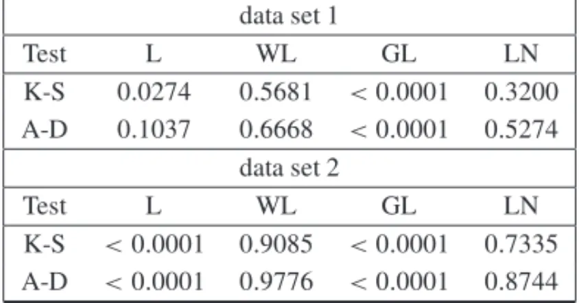
In Table 3 we present, for both data sets, the corresponding p-values to Kolmogorov-Smirnov (K-S) and Anderson-Darling (A-D) goodness-of-fit statistics. From these results, it is clear that the WL distribution provides a good fit to the given data sets. We also consider the Log-Normal distribution (LN) in the data analysis, since this distribution was considered by [14] (data set 1) and by [25] (data-set 2).

Table 3–Kolmogorov-Smirnov and Anderson-Darling goodness-of-fit statistics.

data set 1

Test L WL GL LN

K-S 0.0274 0.5681 <0.0001 0.3200 A-D 0.1037 0.6668 <0.0001 0.5274

data set 2

Test L WL GL LN

K-S <0.0001 0.9085 <0.0001 0.7335 A-D <0.0001 0.9776 <0.0001 0.8744

4 CONCLUDING REMARKS

In this paper we introduced an alternative parametrization for the shape parameter of the weighted Lindley distribution (WL) introduced by [12], which generalizes the one parameter Lindley dis-tribution. In the proposed parametrization, the new parameter have a direct interpretation and it is orthogonal to the shape parameter.

1.6 1.8 2.0 2.2 2.4 2.6

0.014

0.015

0.016

0.017

0.018

0.019

0.020

0.021

β

µ

R = 0.05 R = 0.05

R = 0.20 R = 0.20

R = 0.50 R = 0.50

1.6 1.8 2.0 2.2 2.4 2.6

165

170

175

180

185

190

β

θ

R = 0.05

R = 0.20

R = 0.50

(a) (b)

14 16 18 20

2.2

2.4

2.6

2.8

3.0

3.2

β

µ

R = 0.05 R = 0.05

R = 0.20 R = 0.20

R = 0.50 R = 0.50

14 16 18 20

6.8

6.9

7.0

7.1

7.2

β

θ

R = 0.05

R = 0.20

R = 0.50

(c) (d)

REFERENCES

[1] AKAIKEH. 1983. Information measures and model selection. In: ‘Proceedings of the 44th session of the International Statistical Institute, Vol. 1 (Madrid, 1983)’, Vol. 50, pp. 277–290. With a discussion in Vol. 3, pp. 209–219.

[2] BARNDORFF-NIELSENOE & COXDR. 1994.Inference and asymptotics, Vol. 52 ofMonographs on Statistics and Applied Probability, Chapman & Hall, London.

[3] BEBBINGTON M, LAI C & ZITIKIS R. 2007. Bathtub-type curves in reliability and beyond.

Australian & New Zealand Journal of Statistics,49(3): 251–265.

[4] BJERKEDALT. 1960. Acquisition of resistance in guinea pigs infected with different doses of virulent tubercle bacilii.Amer. J. Hyg.,72: 130–148.

[5] BORAHM & BEGUMRA. 2002. Some properties of Poisson-Lindley and its derived distributions.

Journal of the Indian Statistical Association,40(1): 13–25.

[6] BORAHM & DEKANATHA. 2001. Poisson-Lindley and some of its mixture distributions.Pure and Applied Mathematika Sciences,53(1-2): 1–8.

[7] BORAHM & DEKANATHA. 2001. A study on the inflated Poisson Lindley distribution.Journal of the Indian Society of Agricultural Statistics,54(3): 317–323.

[8] CHENZ. 2000. A new two-parameter lifetime distribution with bathtub shape or increasing failure rate function.Statistics & Probability Letters,49: 155–161.

[9] COXDR & REIDN. 1987. Parameter orthogonality and approximate conditional inference.Journal of the Royal Statistical Society. Series B,49(1): 1–39. With a discussion.

[10] GHITANYME, AL-MUTAIRIDK & NADARAJAHS. 2008. Zero-truncated Poisson-Lindley distri-bution and its application.Mathematics and Computers in Simulation,79(3): 279–287.

[11] GHITANYME & AL-MUTARIDK. 2008. Size-biased Poisson-Lindley distribution and its applica-tion.METRON – International Journal of Statistics,66(3): 299–311.

[12] GHITANYME, ALQALLAFF, AL-MUTAIRIDK & HUSAINHA. 2011. A two-parameter weighted Lindley distribution and its applications to survival data’,Mathematics and Computers in Simulation, 81: 1190–1201.

[13] GHITANY ME, ATIEH B & NADARAJAH S. 2008. Lindley distribution and its application.

Mathematics and Computers in Simulation,78(4): 493–506.

[14] GUPTA RC, KANNAN N & RAYCHAUDHURI A. 1997. Analysis of Lognormal survival data.

Mathematical Biosciences,139: 103–105.

[15] HAUPTE & SCHABE¨ H. 1992. A new model for a lifetime distribution with bathtub shaped failure rate.Microelectronics Reliability,32(5): 33–639.

[16] KALBFLEISCHJG. 1985.Probability and statistical inference. Vol. 2, Springer Texts in Statistics, second edn, Springer-Verlag, New York.

[17] LAI CD, XIE M & MURTHY DNP. 2001. Bathtub-shaped failure rate life distributions. In: ‘Advances in reliability’, Vol. 20 ofHandbook of Statistics.North-Holland, Amsterdam, pp. 69–104.

[19] LANCASTERT. 2002. Orthogonal parameters and panel data.Review of Economic Studies,69(3): 647–666.

[20] LINDLEYD. 1965.Introduction to Probability and Statistics from a Bayesian Viewpoint, Part II: Inference. Cambridge University Press, New York.

[21] LINDLEY DV. 1958. Fiducial distributions and Bayes’ theorem. Journal of the Royal Statistical Society. Series B. Methodological,20: 102–107.

[22] LOUZADAF & CAVALIW. 2014. On a double reparametrization for accelerated lifetime testing.

Chilean Journal of Statistics,5(1): 37–48.

[23] LOUZADA-NETOF & PARDO-FERNANDEZ. 2001. The effect of reparametrization on the accuracy of inferences for accelerated lifetime tests.Journal of Applied Statistics,28: 703–711.

[24] MAHMOUDIE & ZAKERZADEHH. 2010. Generalized Poisson Lindley distribution. Communica-tions in Statistics Theory and Methods,39: 1785–1798.

[25] MART´INJ & P ´EREZCJ. 2009. Bayesian analysis of a generalized lognormal distribution. Computa-tional Statistics & Data Analysis,53: 1377–1387.

[26] MAZUCHELIJ & ACHCARJA. 2011. The Lindley Distribution Applied to Competing Risks Lifetime Data.Computer Methods and Programs in Biomedicine,104(2): 188–192.

[27] MEEKERWQ & ESCOBARLA. 1998.Statistical Methods for Reliability Data. John Wiley & Sons, New York.

[28] NADARAJAHS. 2008. Bathtub-shaped failure rate functions.Quality & Quantity,43(5): 855–863.

[29] OLVERFWJ, LOZIERDW, BOISVERTRF & CLARKCW. (eds.) 2010.NIST Handbook of math-ematical functions, U.S. Department of Commerce National Institute of Standards and Technology, Washington, DC.

[30] RAJARSHIS & RAJARSHIMB. 1988. Bathtub distributions: A review.Communications in Statistics. Theory and Methods,17: 2597–2621.

[31] SANKARANM. 1970. The discrete Poisson-Lindley distribution.Biometrics,26: 145–149.

[32] SAS. 2010.The NLMIXED Procedure, SAS/STATR _{User’s Guide, Version 9.22, Cary, NC: SAS} Institute Inc.

[33] SCHAFFTHA, STATONTC, MANDELJ & SHOTTJD. 1987. Reproducibility of electromigration measurements.IEEE Transactions on Electronic Device,34(3): 673–681.

[34] SCHWARZGE. 1978. Estimating the dimension of a model.Annals of Statistics,6(2): 461–464.

[35] SMITHRM & BAINLJ. 1975. An Exponential Power Life-Test Distribution. Communications in Statistics,4(5): 469–481.

[36] ZAKERZADEHH & DOLATIA. 2009. Generalized Lindley distribution. Journal of Mathematical Extension,3(4): 13–25.