The impact of a “Minimum Guaranteed Income Program” in Portugal
Miguel GOUVEIA
FCEE, Universidade Católica Portuguesa and
Carlos FARINHA RODRIGUES
Abstract
The objective of this paper is to estimate the impact of the Portuguese Minimum Guaranteed Income Program (RMIG). We estimate its impact on the distribution of household incomes and poverty as well as the size of government expenditures necessary to finance the program. The baseline adopted is constructed under the assumption of no behavioural responses to the transfer mechanism and of total participation of all eligible households. The simulation shows that 4,8% of domestic households and 5,7% of the population are eligible to receive the RMIG. The Program has a small but positive impact in reducing inequality. However, taking labour supply effects into account results in a smaller gain in inequality reduction. Similarly, we have a small but positive impact on the poverty rate for individuals. This gain, however, is almost cancelled when labour supply reactions are taken into account. However the most important consequences of the RMIG are sharp gains in the measures of poverty severity and intensity. In these dimensions, taking into account the labour supply incentives of the RMIG does not reduce substantially the positive impacts of the Program.
Keywords: Income Distribution, Inequality, Poverty Alleviation, Social Policy
JEL Classification: D63, I38
Correspondence to:
Miguel Gouveia, Departmento de Economia, Universidade Católica Portuguesa, Palma de Cima, 1600 Lisboa, Portugal. (E-mail: [email protected] )
or
Carlos Farinha Rodrigues, CISEP, Instituto Superior de Economia e Gestão, Rua Miguel Lupi 20, 1200 Lisboa, Portugal (E-mail: [email protected] )
The authors gratefully acknowledge INE (Instituto Nacional de Estatística-Portugal) for having authorised the use of micro-data sets from the household budget surveys.
1. Introduction
In 1996 the government began experiments with localised introductions of a Minimum Guaranteed Income Program (RMIG) in Portugal. After that experimental stage the RMIG had its official beginning as a means-tested universal access program in late 1997.
The main objective of this paper is to present a study of the RMIG effects. We estimate its impact on the distribution of household incomes and welfare as well as the size of government expenditures necessary to finance the program.
The analysis will be carried out in three stages. In the first stage we use the 1995 Household Budgets Survey (HBS95) to establish a baseline. Initially we operationalize basic concepts such as the definition of total household income, earnings, income from capital, and government transfers. We also have to establish appropriate equivalence scales. Finally, we estimate a central case poverty line, as well as a few alternatives to this central case.
Once these steps are taken we target the individual distribution of equivalent income as the basic object of analysis. We characterise the baseline scenario along several dimensions: an array of inequality measures (Gini, Atkinson, and Generalised Entropy (GE), these last two with several inequality aversion parameter values; an array of Poverty Measures including the poverty rate, the poverty gap, and other Foster’s measures (F).
In a second stage we introduce the parameters of the RMIG Law into a calculator that maps household demographic characteristics and income (total and composition) into transfers. Next, we simulate the distribution of income resulting from the program. This is done under the assumption of no behavioural responses to the transfer mechanism and of total participation of all eligible households. After this simulation is carried out, the analysis proceeds in two directions. One is to characterise the resulting income distribution exactly in the same way as we did in the first stage. Then, we can systematically examine the differences in indicators of inequality and poverty. These differences are our measures of the outcomes of the RMIG Program. The second direction is to compute the total amount of transfers for the HBS95 sample and to infer from this the total amount of public expenditures involved in the national implementation of the RMIG program.
The third stage refines the analysis by considering the possibility of behavioural changes induced by the transfers of the RMIG. Here, the analysis will be more tentative as there is little information and scientific literature concerning labour supply in Portugal. The
HBSs have only some information on labour market participation and no information at all regarding hours or any other intensive margin measure of labour supply. In this section we will combine information from the HBS database with the information from empirical labour supply analyses performed for other countries to estimate the effects of the RMIG on the labour supply of the households. We anticipate little or no response from households with elderly or handicapped members, but we have very imprecise priors on what the response sizes for other households might be.
2. The Departure point
In order to assess the impact of the introduction a Minimum Guaranteed Income Program in Portugal we begin by an examination of the distribution of income and the extent of inequality and poverty before the implementation of the Program.
The Household Budget Survey, conducted by the Portuguese Statistical Office (INE) in 1994/95, will be used as the base dataset to characterise the departure situation in terms of income distribution. It has a structure similar to the earlier HBSs studied in Gouveia and Tavares (1995), Gouveia and Albuquerque (1994), Rodrigues (1993,1994,1996), Costa (1994) and Ferreira (1992).
The sample consists of 8130 households which have been select in order to be representative of the whole population.
The definition of disposable income used in this survey is very comprehensive: it includes income from earnings, investment income, transfer and capital receipts, income in kind as production for home consumption and imputed rents. Income is net of taxes and of social security contributions. The OECD scale is used to deflate the household incomes and to obtain the equivalent income of each individual in the household.(1). The price level was updated to 1996, the year for the construction of the Baseline Scenario and the departure point to all simulations.
Table 1 portrays the individual distribution of equivalent income by deciles. It presents the mean income, decile shares and cumulative shares for each decile. The last column shows the decile distribution expressed as percentages of the median income.
(1)
The equivalent scale recommended by the OECD is 1 for the first adult, 0.7 for other adults and 0.5 for children aged less than 14.
Table 1
Portugal 1996 – Individual distribution of equivalent income, by Decile
Decile Decile Mean Income Decile Shares Cumulative Shares Mean Income as % of Median 1 358,30 0,03023 0,03023 38,19 2 528,36 0,04469 0,07492 56,31 3 652,14 0,05501 0,12992 69,51 4 759,38 0,06439 0,19432 80,94 5 876,36 0,07386 0,26817 93,40 6 1011,26 0,08576 0,35394 107,78 7 1170,21 0,09871 0,45265 124,72 8 1398,42 0,11825 0,57089 149,05 9 1807,95 0,15281 0,72371 192,69 10 3261,30 0,27629 1,00000 347,59 All 1170,95 124,80
Summary measures of inequality2 are presented in Table 2. The Gini Index shows a value of 34.8%, a large number by comparison with other European countries.
Table 2
Portugal 1996 – Summary Measures of Inequality
Gini 0.34797 Atkinson (ε= 0.5) 0.09871 Atkinson (ε= 1) 0.18190 Atkinson (ε=2) 0.31900 Entropy (α=0) 0.20077 Entropy (α=1) 0.21634
Finally table 3 summarises the findings regarding poverty using different poverty lines computed as 40%, 50% and 60% of median income. Focusing on the 50% line, a
2 For detailed informations on these measures see Atkinson (1970,1983), Cowell (1981,1994)
standard first proposed by Fuchs (1967), the table reveals that around 10% of the population can be considered as poor.
Table 3
Portugal 1996 – Poverty Measures
% of the Median 40% 50% 60% Poverty Line 375,54 469,43 563,31 F0 - Head Count 0,04823 0,10499 0,17523 F1 - Severity 0,01091 0,02367 0,04314 F2 - Intensity 0,00411 0,00873 0,01622
3. Methodology to build the different scenarios: The Baseline Scenario
The construction of the Baseline Scenario constitutes a decisive step in modelling the impact of the introduction a Minimum Guaranteed Income Program. The main objective is to try to reproduce the legal framework established by the Law that creates the Program. It identifies the households that are eligible to receive the minimum income, the amount of the subsidy that each household will receive and the total cost of the Program.
The main stages in building the Baseline Scmnario can be synthesised as follows:
i) Construction of the equivalence scale underlying the RMIG legislation. The equivalence scale established by the RMIG Law is very close to the OECD scale but it weights differently the second adult in the household.
ii) Identification of the “minimum income” for each household in the dataset. This basic income is computed multiplying the value of the Social Pension in 1996 (20000 escudos) by the number of equivalent adults (RMIG scale) existing in each household;
iii) Construction of the “reference income” of each household. This is the income that serves as a reference for the determination of the RMIG eligibility. The reference income is obtained by the aggregation of all monetary sources of income of the household but where only 80% of the wages and salaries are included;
iv) Identification of households that are eligible to receive the subsidy. Any household whose reference income is less than its defined minimum income will
automatically be included in the Program;
v) Determination of the annual subsidy for each household in the program. The subsidy that each household receives is equal to the difference between the minimum income calculated for this household and its reference income;
vi) Construction of the post-transfer income distribution. This distribution is built from the initial one by adding up the amount of the RMIG transfers to all eligible households.
The Baseline Scenario is constructed under the assumption that there are no behavioural responses to the transfer mechanism. The assessment of the impact of the RMIG will be done by comparing the original distribution of income (pre-RMIG distribution) with the one that results from the application of the Program (Post-RMIG distribution.
The differences between the two distributions, in terms of inequality and poverty, can be interpreted as the outcome of the RMIG Program. This is done using the range of methods and indicators of presentation of the distribution described in the previous sections. The main questions that we try to answer are: who benefits the most from the program, what are the costs associated with its implementation, what are its effects on inequality and poverty.
Table 4 summarises the main macroeconomic outcomes of the application of the program. It shows that 4.8% of the total households and 5.7% of the total population have an income low enough to be entitled to the RMIG. One first conclusion that we can draw from the figures is that only half of the people in poverty (with the poverty line established as 50% of the median income) will benefit from the program.
Table 4
Baseline Scenario – Macroeconomic Indicators
Household Participation Rate 150170 (4.8%)
Individual Participation Rate 533514 (5.7%)
Total Program Expenditure (109 escudos) 30.575 Mean Household Transfer ( 103 escudos ) 203.6
The program implies a public expenditure in transfers of 30.6 x 10⁹ escudos (1996 prices). This amounts to 0.18% of the Portuguese 1996 GDP and 0.39% of the 1996
total public expenditures3. The mean household transfer is 203.6 thousand escudos, which represents an average increment of 18.5% in annual income of the households involved in the program.
Table 5 gives us a first picture of the distributional effects of the RMIG transfers, showing the households receiving these transfers where are located in the distribution. The RMIG has an important effect over the share of total income detained by the first decile that increases by more than 2 percentage points. After the fourth decile the effects are not significant.
Table 5
Lorenz Curves - Impact of the RMIG Program Decile Pre-RMIG Post-RMIG Variation (%)
1 0.03023 0.03279 8.47% 2 0.07492 0.07782 3.88% 3 0.12992 0.13288 2.27% 4 0.19432 0.19700 1.38% 5 0.26817 0.27094 1.03% 6 0.35394 0.35611 0.61% 7 0.45265 0.45445 0.40% 8 0.57089 0.57264 0.31% 9 0.72371 0.72470 0.14% 10 1.00000 1.00000
Tables 6 and 7 illustrate the effectiveness of the RMIG as an instrument to reduce inequality and poverty, as a factor to improve the well being of the population. Table 6 shows that the RMIG as a small but positive impact in inequality. All the indices present a reduction of the inequality levels, but the indices that are relatively more sensitive to changes at the bottom of the distribution register larger reductions.
Table 6
Inequality Measures - Impact of the RMIG Program
Pre-RMIG Post-RMIG Variation (%)
Gini 0.34797 0.34378 -1.20% Atkinson (ε= 0.5) 0.09871 0.09568 -3.10% Atkinson (ε= 1) 0.18190 0.17439 -4.13% Atkinson (ε=2) 0.31900 0.29545 -7.38% Entropy (α=0) 0.20007 0.19163 -4.55% Entropy (α=1) 0.21634 0.21137 -2.30%
The results of the application of the Guaranteed Minimum Income Program in terms of reduction of poverty are displayed in table 7. Taking the poverty line defined as 50% of the median income we find that the RMIG has a slight impact on the poverty rate. This is not an obvious result because the RMIG level per adult is about 52% of the poverty line and thus one would not expect to have any households pushed above that line. However, we have to keep in mind that the reference income used to define the income transfers under the RMIG law does not coincide with our much more comprehensive income definition. A result of this discrepancy is that some households with comprehensive income close to the poverty line are nevertheless eligible to receive transfers under RMIG, an event that explains the positive impact of the RMIG on the poverty rate. The number of individuals on poverty reduces from 10,5% of the population to 9,8%. Although this reduction seems very modest it implies that around 21000 households and more than 66000 persons leave poverty.
Table 7
Poverty Measures - Impact of the RMIG Program
Pre-RMIG Post-RMIG Variation (%)
Poverty Line (40% of Median Income) 375.54 375.54
F0 - Head Count 0.04823 0.03658 -24.15%
F1 Severity 0.01091 0.00464 -57.47%
F2 Intensity 0.00411 0.00086 -79.12%
Poverty Line (50% of Median Income) 469.43 469.43
F0 - Head Count 0.10499 0.09795 -6.71%
F1 Severity 0.02367 0.01702 -28.08%
F2 Intensity 0.00873 0.00428 -50.98%
Poverty Line (60% of Median Income) 563.31 563.31
F0 - Head Count 0.17523 0.17201 -1.84%
F1 Severity 0.04314 0.03667 -15.00%
More significant than the reduction on the incidence of poverty are, however, the alterations in the severity and in the intensity of the poverty4. The effectiveness of the program in reducing the severity (F1) and the intensity (F2) of poverty are impressive (respectively, 28% and 51%). Those figures imply that the RMIG Program could have a very positive effect in reducing situations of extreme poverty.
5. The RMIG and the Incentive Effects on Labour Supply
Introduction
The previous quantitative analysis on the implementation of the RMIG assumed the program would not have a significant effect on economic behaviour. This section presents a refinement of the analysis where we take predictable changes of behaviour into account.
From an economic point of view the areas that may be considered more important include labour supply5, the intensity of effort in job search, investment in human capital, saving, risk taking, etc. Here, we will concentrate solely on what is arguably the most important area: labour supply.
Ideally, the simulation of the changes of behaviour generated by the RMIG should be made relying on a structural econometric model of labour supply. However, we resorted to a less ambitious simulation methodology to create scenarios that captured the labour supply reaction to the RMIG. This methodology rests in the parameterisation of labour supply functions with estimates of the wage and exogenous income labour supply elasticities. The key point is that the methodology used does not need any information on hours of work, a feature required to use the household survey data since the survey does not have information on any measure of labour supply such as hours per week or even days per year.
The methodology also assumes that there is no rationing of labour supply on the demand side of the labour market and that the RMIG does not modify the productivity of the potential workers.
There is a question that is not dealt with in this paper. The RMIG may involve mandatory work or training. Naturally, the idea is that these requirements both serve as a screening device and as a forced investment in human capital that will facilitate an exit
4For details on these measures see Sen (1979,1997),
Foster, J., Greer, J. and Thorbecke, E. (1984) or Ravallion (1994).
5
out of poverty. However, in so far as these work and training requirements cause an additional reduction in market labour supply the RMIG becomes a more expensive program. In that sense the requirements will add to the disincentive effects generated by the transfers and to lead to additional reductions in labour market effort.
The basic model
The specification starts with a standard linear regression explaining labour supply with coefficients β and the following variables:
H hours worked
w, is the net wage rate
τ is the tax on wages I exogenous income X other relevant variables.
H = β0 + β ω1 + β2 I + β3 X
From the previous equation we find the percentage change in labour supply due to net wage and exogenous income changes:
∆ H ∆ ∆ H I I =
π
ω
+ω
π
1 2where π1 is the wage elasticity and π2 is the exogenous income elasticity: π1 = β ω H π β 2 = I H
The percentage change in the net wage rate due to RMIG is
∆ ω
ω
≈ −
τ
∆H H Rmig y Rmig y e e = − + − + π τ1 π2 0 0 2 ( ) / ,
where ye0 is the initial exogenous income of the household. The analysis maintains the assumption that participation in the RMIG does not affect the gross wage rate in any way, implying that the percentage change in total earnings is the same as in hours worked.
Killingsworth (1983, p. 119-125, p. 193-199, p. 202), shows that the estimates in the literature vary greatly and that there is a systematic difference between men and women. Thus, it is reasonable to admit that the uncompensated wage elasticity of labour supply is in the neighbourhood of 0,1- 0,2 for men and 0,3 - 0,4 for women. We will use several assumptions but will consider a baseline scenario with an elasticity of 0.2. As for the exogenous income elasticity, we have that the literature also displays reasonable amplitude of estimates, again with a systematic difference between men and women. We will perform simulations assuming alternative values for this parameter considering a baseline of - 0.15.6
One final issue that needs to be considered in the programming of the simulations is the existence of incomes that are not considered as such by the rules of the RMIG. This is the case of the implicit incomes in owner-imputed rents and production of foodstuffs for own consumption. The handling given to these incomes in the modelling was to include them as exogenous income relevant to determine the variation in labour supply but obviously, not to include them in the computation of the RMIG for each family unit.
Non-convexities and endogenous program participation
A last problem is modelling the participation in RMIG. It is obvious that households with initial total incomes below the RMIG threshold are eligible to participate. It is equally obvious that households with exogenous incomes above the RMIG will never be eligible. The question is to what extent will households reduce their market labour supply in order to become eligible to participate in the RMIG. An analytical handling of this problem is not trivial.
6
The elasticities are needed to predict the changes in labour income of all eligible households. These changes depend on changes in hours but also of changes in effort intensity, types of jobs (less demanding jobs pay lower wages), etc.. When choosing values for the elasticity parameters all these aspects of labour supply should be taken into account
Figure 1 G r o s s I n c o m e F r o m W o r k C o n s u m p t i o n R M I G a b x z
Hausman (1980, 85) and others have shown that programs with a transfer/benefit structure of the kind found in the RMIG generate a nonconvex budget restriction as illustrated in Figure I. This nonconvexity increases the difficulty in modelling participation in the program.
A lower limit on participation
The static participation case corresponds to assuming that the RMIG does not have any effect on endogenous participation, i.e., that nobody with initial total income above the RMIG decreases labour supply so as to become eligible. This case implies that the participation rates will be minimal. In more formal terms, consider a household with initial labour income yl0 and exogenous income y
e
0. The lower labour income limit for non participation is yl0 * 0.2 + y e 0 > RMIG, or y > 1.25 * (RMIG - y ) l 0 e 0
Figure 1 illustrates a situation where this lower limit is not accurate. An individual in a before RMIG situation chooses to work just enough to have an income equal to the eligibility level. Given the existence of the RMIG she will chose to reduce hours of work and become eligible to the program.
Upper limit on participation
The maximum participation scenarios correspond to recomputing the labour incomes for all those with exogenous income below the RMIG assuming that they participate in the program. After this simulation of the impact of the RMIG on labour supply we verify if
the simulated total income is larger than the eligibility threshold given by the RMIG plus 20% of these gross labour incomes of the work. If that is the case, then the household does not have any advantage in participating in the RMIG, and our calculations place it outside the program. Otherwise the household participates in the RMIG.
Using equation (4) above we compute a percentile reduction of the worked hours ∆H/H. The upper limit labour income for non-participation in RMIG, calculated for each household in the database, is given by (1+∆H/H) * yl0 + ye0 > RMIG +0.2 * yl0 (1-∆ H/H), i.e. y > 1.25 * (RMIG - y ) (1 + H / H l 0 e 0 ∆ )
If the participation condition is met, i.e. earnings are smaller than the threshold above, the transfer T from the RMIG program to the household will be given by
T = Rmig - (0.8 ( 1+∆H/H) * yl 0+ y
e 0).
This equation also applies to the previous scenario, but in that case only to those households with earnings below the threshold defined for that case.
This second case errs on the other side of the previous case, setting thresholds too high and inflating participation rates. Figure 2 shows that some households included in the RMIG according to this rule would actually choose to be outside.7
An "ad hoc" intermediate participation estimate
It is easy to see that both the previous scenarios will err in their accounting for participation in the program. The first sets a threshold too low, both in terms of income and in terms of the implied participation rate. Clearly there will be households with higher incomes that will choose to reduce labour income so as to benefit from the program.
7Graphs 1 and 2 show the same budget constraint but each set of indifference curves comes
Figure 2 G r o s s I n c o m e f r o m W o r k C o n s u m p t i o n R M I G a b x z
A rigorous solution to the problem involves specifying a utility function and have the choice formalised as picking the situation with the highest level of utility. That would require information on wage rate and hours that is not available. The methodology we ended up using has a "ad hoc" nature: we took the threshold level of labour income to be the average of the two thresholds defined previously, or:
∆H/H + 1 0.5 + 0.5 ) y -(RMIG * 1.25 > yl0 e0 .
In this scenario the transfers will be given by the same equation as in earlier scenarios with the sole difference being that it only applies to households with incomes under the
threshold ab o v e.
The Results
Numerous scenarios were simulated taking into account a variety of values for the key elasticity parameters and for the modelling of the participation decision. As one would expect the amount spent in transfers and the participation rates of individuals and households all increase the larger the elasticity parameters assumed. Simulations using the upper limit on participation (not shown) have lower mean household transfers than the other scenarios with behaviour changes because they place households in the program that are closer to the eligibility income limits and that therefore receive small transfers.
Below, we report a selection of the results obtained with the intermediate assumptions on participation. Occasionally we will make reference to results not shown for reasons of space but available by request.
Table 8
Simulation with Incentives –Intermediate Level of Participation
Baseline A B C D E
Wage Elasticity 0 0.2 0.3 0.2 0.1 0.08
Exogenous Income Elasticity 0 -0.15 -0.15 -0.2 -0.1 -0.1
Total Program Expenditure ( 109 escudos) 30.6 56.8 71.0 67.0 41.6 40.3
Household Participation Rate (%) 4.78 7.21 8.30 8.02 5.81 5.66
Individual Participation Rate (%) 5.67 8.87 10.20 9.88 7.01 6.83
Mean Household Transfer (103 escudos ) 203.6 250.7 272.0 265.2 227.9 226.6
The results above show that direct expenditure and participation rates can double in the scenarios with larger elasticities. Even in the more conservative cases the explicit introduction of behaviour has sizeable effects.
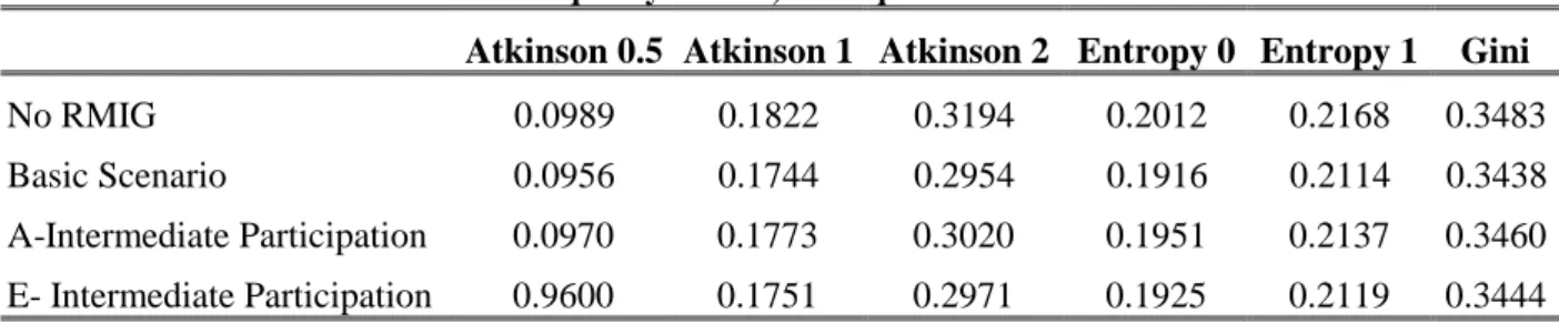
Table 9 shows the impact of the program in a set of inequality indices. Including the labour supply responses reduces the RMIG gains in inequality reduction by comparison with estimates assuming no behavioural changes, but there is still a gain when the comparison is made with reference to the no RMIG scenario. 8
Table 9
Incentives and Inequality Indices, Net Equivalent Incomes
Atkinson 0.5 Atkinson 1 Atkinson 2 Entropy 0 Entropy 1 Gini
No RMIG 0.0989 0.1822 0.3194 0.2012 0.2168 0.3483 Basic Scenario 0.0956 0.1744 0.2954 0.1916 0.2114 0.3438 A-Intermediate Participation 0.0970 0.1773 0.3020 0.1951 0.2137 0.3460 E- Intermediate Participation 0.9600 0.1751 0.2971 0.1925 0.2119 0.3444 8
Cases with large elasticities and upper limit participation levels have indices of inequality that are larger with the RMIG than in the no RMIG case.
Poverty measures respond in much the same way as inequality indexes, as Table 11 shows.
Table 10
Incentives and Poverty Indices, Net Equivalent Incomes F0 Head Count F1 Severity F2 Intensity No RMIG 0.1058 0.0238 0.0088 Basic Scenario 0.0980 0.0170 0.0043 A-Intermediate Participation 0.1047 0.0204 0.0055 E- Intermediate Participation 0.0987 0.0178 0.0046
Comparing the situation without RMIG and the simulations with intermediate participation rates, there is a small reduction in the prevalence of poverty. One notices, however, that the poverty rates were uniformly lower when incentive are ignored. Simulations with larger elasticities and using the upper limit for participation show that in such an extreme case the poverty rate can be even larger than in the no RMIG scenario.
However, if the positive impact on poverty rates can be diminutive and in extreme cases reversed the positive impact on severity (the poverty gap) is proportionally larger. Finally, the impact on intensity is not only larger but also not reversed even in the most extreme cases simulated.
These results legitimise a conclusion: the RMIG may not be very effective in diminishing the number of the poor in Portugal, but it will certainly have a large and positive impact in reducing the situations of extreme poverty.
6. Conclusions and suggestions for research
Main results
This paper reported exploratory work with the purpose of evaluating the impact of the Portuguese Minimum Guaranteed Income program on the inequality of the income distribution, on poverty levels and its consequences in terms of public expenditures.
The baseline adopted to estimate the impact of the Guaranteed Minimum Income (RMIG) is the distribution of the income in 1995 from the Household Budget Survey. Estimates for a no-behaviour-changes scenario are that 4,8% of domestic households and 5,7% of the people are eligible to receive the RMIG with a public expenditure in transfers with the amount of 30.6 × 10⁹ escudos (1996 prices).
The paper then deals with program induced changes in behaviour namely changes in labour supply. A variety of cases are studied. In the simulation considered to be most reliable results show that 7,2% of households and 8,9% of the people are eligible to participate in the RMIG. If all the eligible households participate, the expenditure with the transfers amounts to 56. 8 × 10⁹ escudos.
The Minimum Income Guaranteed program has a small but positive impact in reducing inequality. Before the program the Gini of the individual distribution of equivalent income is 0.348 and after the program it goes to 0.344 if no behavioural changes occur. However, taking labour supply effects into account the gain in inequality reduction is smaller and in the reference scenario the Gini reaches a value of 0.346. Similarly, we have a small but positive impact in the poverty rate for individuals that goes from 10.6% before RMIG to 9.8% after. This gain, however, is almost cancelled when labour supply reactions are taken into account since the estimated rate after the RMIG becomes 10.5%. Naturally, these weak results are linked to the difference between the estimated relative poverty line (470 × 103 escudos) and the minimum guaranteed income proper, (240× 103). However, to evaluate the RMIG for its impact in the poverty rates alone is to lose its most important positive impact. The most important consequences of the RMIG are sharp gains in the measures of poverty severity and intensity (F1 and F2). In these dimensions, despite somewhat lessened impacts, taking into account the labour supply incentives of the RMIG do not reduce substantially the positive impacts.
Further research
The exploratory nature of this work revealed some areas where there are large gaps in our knowledge that should be covered. This could be feasible as the administrative records of the program and labour supply surveys become available to the research community allowing for work as in Kershaw (1976,1977), Hausman and Wise (1985) or Munell (1986).
The first gap relates to the “take-up” of the program. The quantitative analysis presented assumed that all RMIG eligible households participate in the program and receive the transfers specified. This is an approach that needs to be refined since the percentage of
the eligible people that will in fact apply to the program will likely be significantly below 100%.
The second gap is the absence of a structural econometric model for labour supply. If the necessary data becomes available it will be possible to estimate such a model. Its availability would help to perfect the estimates in this paper and permit a rigorous analysis of policy changes, such as increasing the eligibility thresholds or lowering the implicit marginal tax rates.
The third gap relates to dynamics. Ultimately, the goals of the RMIG program are not only to alleviate poverty but also to help households escape from it. To look at this question we need a dynamic analysis of how participation in the RMIG affects the hazard rates of entry into poverty and exit from it.
REFERENCES
Atkinson, A. B. (1970) "On the Measurement of Inequality," Journal of Economic Theory, 244-63.
Atkinson, A. B. (1983), The Economics of Inequality (2nd Ed).
Atkinson, A.B., T. Smeeding. (1995), “Inequality in OECD Countries”, OECD, Social Policy Studies nº 18.
Burtless, G. and J. Hausman (1978), “ The effect of taxes on labour supply: Evaluating the Gary Negative Income Tax Experiment”, Journal of Political Economy, 86.
Costa, A. Bruto da (1994), "The Measurement of Poverty in Portugal", Journal of European Social Policy, 4, 2, 95- 115.
Cowell, F. (1981), Additivity and the Entropy Concept: an Axiomatic Approach to Inequality Measurement”, Journal of Economic Theory, 25(1), August 1981
Cowell, F. (1984), “The structure of American Income Inequality”, Review of Income and Wealth; 30(3) September 1984
Cowell, F. (1994), Measuring Inequality, LSE Handbooks in Economics, London2ª Ed. Ferreira, L. (1992), “Pobreza em Portugal - Variação e Decomposição de Medidas de Pobreza a partir dos Orçamentos familiares de 1980-1981 e 1989-1990”, Estudos de Economia, 12, 4, 377-393
Foster, J., Greer,J. and Thorbecke,E. (1984), “A Class of Decomposable Poverty Measures”, Econometrica; 52(3), 761-66.
Fuchs, V. (1967), “Redefining Poverty and Redistributing Income”, The Public Interest, 8, 88-95.
Gouveia, M, J. Tavares (1995), "The Distribution of Household Income and Expenditure in Portugal: 1980 and 1990", Review of Income and Wealth, Mars.
Gouveia, M., R. Albuquerque (1994), “A Distribuição dos Salários em Portugal: 1980 e 1990”, Boletim Trimestral do Banco de Portugal, Março.
Hausman, J. (1980), Labour Supply, in: Eds. H. Aaron e J. Pechaman (1980), How Taxes Affect Economic Behaviour, Brookings.
Hausman, J. (1985), Labour Supply, in (Eds.) Feldstein e Auerbach, Handbook of Public Economics, North-Holland.
Hausman, J., D. Wise (1985), Social Experimentation, Chicago, University Press. Kershaw, D. (Ed.) (1976-1977), The New Jersey income-maintenance experiment Vols. I, II e III. New York, Academic Press.
Killingsworth, M. (1983), Labour Supply, Cambridge University Press.
King, M. (1983), “Welfare Analysis of Tax Reform using Household Data”, Journal of Public Economics, 21, 183-215.
Lambert, Peter (1993), The Distribution and Redistribution of Income. A Mathematical Analysis, 2nd ed. (Manchester: University Press).
Munnell, A. (Ed.), (1986), Lessons from the income maintenance experiments, Boston, Federal Reserve Bank of Boston.
Moffitt, R. (1992), “ Incentive Effects of the U.S. Welfare System: A Review”, Journal of Economic Literature, 30, 1, 1-61.
Ravallion, M. (1994), Poverty Comparisons, Harwood Academic Publishers, Chur Switzerland.
Rodrigues, C.F. (1993), The Measurement and Decomposition of Inequality in Portugal [1980/81 - 1989/90]“, Microsimulation Unit Discussion Paper MU9302, Cambridge, Department of Applied Economics.
Rodrigues, C. F. (1994), “Repartição do Rendimento e Desigualdade: Portugal nos anos 80”, Estudos de Economia, 14, 4, 399-427.
Rodrigues, C.F. (1996), “Medição e Decomposição da Desigualdade em Portugal [ 1980 - 1990]“, Revista de Estatística, vol. 1 nº 3.
Sadka, E. (1976), “On Income Distribution, Incentive Effects and Optimal Income Taxation”, Review of Economic Studies, 43, 261-268
Sen, A. (1979), “Issues in the measurement of poverty,” Scandinavian Journal of Economics, 285-307.
Sen, A. (1997), On Economic Inequality, Expanded Edition with a Substantial Annexe by James Foster and Amartya Sen, Clarendon Paperbacks