Equity valuation using accounting numbers in low and high Beta Firms

(1)

I

Lancaster University Management School

Department of Accounting & Finance

Equity Valuation Using Accounting Numbers

in Low and High Beta Firms

Candidate:

Pedro Miguel Coutinho

Supervisor:

Dr. Geraldo Cerqueiro

September 2013

This dissertation is submitted in partial fulfilment of degree of

Master of Science in Finance

(2)

(3)

III

Abstract

The aim of this paper is to study the performance of different accounting valuation models across firms with different beta levels. In order to create this analysis more realistic, both sub samples will be distinguished, according to their leverage level, in quartiles.

Initially, not only several studies developed concerning equity valuation using accounting-based valuation models, which will provide an important theoretical support to this analysis, but also a brief reflection on the relevance of the variable beta will be introduced. Then, stock-based and flow-based accounting valuation models are analyzed across low beta firms and high beta firms. While valuation models on low beta firms perform better when selected companies with extreme leverage levels, when applied for companies with average leveraged levels, these same models show better results on high beta firms.

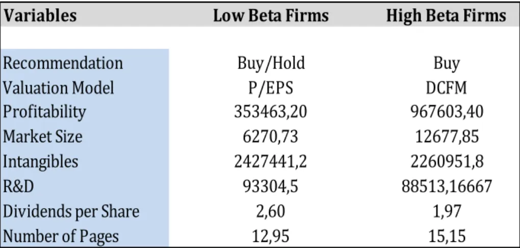
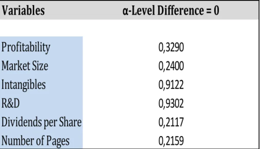
In order to understand whether analysts take into consideration the results provided by the previous analysis, a small sample analysis, applied for some UK companies with different beta values, examines not only the investment recommendations and the valuation models used in practice by brokers’ reports, but also other relevant variables, such as, the firm’s profitability, market size, intangible-intensity, R&D expenses and the number of pages per broker report.

(4)

IV

I Table of Contents

...

IV

II List of Tables

...

VI

III Abbreviations

...

VII

1. Introduction...1

2. Review of Relevant Literature...2

2.1. Usefulness of Equity Valuation...2

2.2. Usefulness of Accounting Numbers...3

2.3. Valuation Models...5

2.3.1. Perspectives of Valuation...5

2.3.2. Stock Based Valuation Model...5

2.3.2.1. Selection of Comparable Firms...6

2.3.2.2. Computing the Benchmark Multiple...8

2.3.2.3. Selection of the Value Driver...8

2.3.3. Flow Based Valuation Models...9

2.3.3.1. Dividends Discount Model...9

2.3.3.2. Discounted Free Cash-Flow Model...11

2.3.3.3. Residual Income Valuation Model...13

2.3.3.4. Ohlson Juettner-Nauroth Model...15

2.4. Valuation Models Performances...16

2.5. Review of Literature of Beta Variable...18

3. Large Sample Analysis...21

(5)

V

3.2. Research Question...22

3.3. Research Design...22

3.3.1. Data and Pooled Sample Selection...22

3.3.2. Valuation Models...23

3.4. Empirical Results...25

3.4.1. Descriptive statistics...25

3.4.2. Significant Level Tests between Sample Partitions...28

3.4.3. Significant Level Tests between valuation models...29

3.4.4. Power of Valuation Models...30

3.4.5. Robustness Test...31

3.5. Concluding Remarks...34

4. Small Sample Analysis...36

4.1. Introduction...36

4.2. Hypothesis development...36

4.3. Research Design (Sample and Data)...38

4.4. Empirical Evidence...40

4.4.1. Descriptive Statistics...40

4.4.2. Significant Level tests...42

4.5. Concluding Remarks...43

5. Conclusion ...44

(6)

VI

II - List of Tables

Table 1 – Sample Data Selection...23

Table 2 – Sub Sample Division...23

Table 3 - Descriptive Statistics: Valuation Errors...26

Table 4 – Comparison of Prediction Errors between Sample Partitions...28

Table 5 - Models valuation performance...29

Table 6 – Explanatory power of valuation models...31

Table 7 – Robustness Test...32

Table 8 – Explanatory Power of Valuation Models...33

Table 9 – Sample Selection...39

Table 10 – Descriptive Statistics...40

(7)

VII

III - Abbreviations

Abnormal Income Growth Book Value of Equity Book Value

Firms’ Beta

Capital Expenditures Cash Flow

Cash Flow From Investment Activities

Cash Flow From Operations Clean Surplus Relationship Discounted Cash Flow

Discounted Cash Flows Model Dividends Discount Model Dividends

Equity

Earnings P/Share

Earnings Before Interest and Taxes

Earnings Before Interest, Taxes, Depreciations and Amortizations Enterprise Value

Free Cash Flow Growth Rate

Generally Accepted Accounting Principles

Initial Public Offering

International Financial Reporting Standard AIG BV CAPEX CF CFI CFO CSR DCF DCFM DDM DIV E EPS EBIT EBITDA EV FCF g GAAP IPO IFRS Cost of Debt Cost of Equity Market Value Median Mean

Merger and Acquisitions Net Operating Assets

Net Operating Assets after Taxes Net Income

Net Working Capital

Ohlson Juettner-Nauroth Model Operating Income

Price to Book Ratio Price-Earnings Ratio P-Value

Quartile 1 Quartile 3

Research & Development Risk Free Rate

Residual Income Valuation Model Market Return

R-Squared

Standard Deviation Tax Rate

Market Value of Debt Market Value of Equity

Weighted Average Cost of Capital kd MV MD MN M&A NOA NOPAT NI NWC OJM OI P/ B PER pv Q1 Q3 R&D Rf RIVM Rm SD Tc WACC

(8)

1

1. Introduction

The main aim of this paper is to study the performance of different accounting valuation models of firms with different beta levels. Having the main objective drawn, it will also be relevant to study the possibility of possible dissimilarities across low and high beta firms.

To begin with, as regards the large sample analysis, a large sample of low and high beta non-financial firm values will be estimated using four different accounting valuation models. To provide the reader with a more realistic analysis, sample data were grouped, in the first place, into quartiles according to the companies’ leverage value and, only then, distinguished in two categories: low and high beta firms. For each of these sub samples, preferential accounting valuation models were selected according to their valuation errors and explanatory power.

After this, we will take a small sample analysis in order to verify if the results given in the previous analysis are applied and used by analysts or not. At this point, not only several brokers’ reports but also other sources of information will be carefully observed and discussed for each of the two sub samples in order to understand if valuation models users apply different valuation models in practice. In addition to this, other relevant variables, which were collected from several databases, will also be studied in order to identify possible dissimilarities among the set of these sub samples.

As regards the structure of this thesis, the first section gives a brief introduction of what will be discussed throughout the all paper, raising and explaining the relevance of the research question in study: the performance of different accounting valuation models on firms with different beta levels. The following section will present not only several studies developed concerning equity valuation using accounting-based valuation models, which will provide an important theoretical support to our analysis, but also a brief reflection on the relevance of the variable beta. In the next section, a large sample analysis will be

(9)

2 presented and empirical results will be carefully discussed. After this section, a small sample analysis will be provided, where several brokers’ reports of a selected sample of companies will be taken into consideration, in order to compare, on the hand, the results given in the large sample analysis with the techniques applied by practitioners, and, on the other hand, to study other relevant variables across these two sub samples. Finally, a conclusion will be drawn exposing the main results obtained from both analysis and some possible suggestions to further relevant researches will be added.

2. Review of Relevant Literature 2.1 Usefulness of Equity Valuation:

Nowadays, it is an undeniable fact that valuation process is a crucial technique that is present in almost every financial decision that has to be made.

To begin the analysis of this topic, it is important to look at the purpose of equity valuation and what it must be meant by equity valuation.

As some important theorists have argued, in simple terms, equity valuation can be described as the actualization process of the forecast expected payoffs to shareholders (Lee, 1999).

It is possible to account two different perspectives to value a firm, the entity perspective and the equity perspective. As regards the first one, it does not take in consideration the capital structure of the firm, valuing, on the contrary, the firm as an all, independently of its source of funding. On the other hand, the second perspective can be described as an equity perspective which only focuses its attention on the capital provided by equity holders and consequently ignores the capital provided by debt holders. Thus, through this perspective, the capital structure is taken into account. (Citigroup Global Markets, 2008)

(10)

3 We must add that the purpose of equity valuation is linked with many different reasons. Generically, the main purposed is linked with the need of quoted share prices, transforming forecasts of key variables into a value estimate (Penman, 2003).

However, the motivations beyond this purposed assume many different rolls. Not only the private companies that want to go public, but also the ones that are under an acquisition process, need to be valued. Moreover, and even though that markets are assumed to be efficient, some firms can be wrongly priced, and so, in order to check that, a valuation process is needed. (Damodaran, 2013) (Malkiel, 1989)

Throughout this section, it will be first presented a short reflection regarding the usefulness of accounting income numbers that will introduce an extensive explanation of different accounting valuation models.

2.2 Usefulness of accounting numbers:

“Valuation is as much an art as it is a science”. (Lee, 1999)

To begin the analysis of this topic it is important to highlight that equity valuation is a rigorous process that requires special attention to various relevant details. Accounting data is considered one of the most precious tools for investors and, when combined with other tools, provide a strong source of information on a particular firm. Although this information does not provide all the tools needed to correctly estimate the intrinsic value of an asset, it gives a relevant help to the valuation’s process.

Taking this important fact into consideration, and in order to create the right conditions for a realistic estimation, analysts should not only be very familiar with this data, but also understand how to deal with it. Hence, it is expected that the information content in accounting numbers is correctly represented by the stock prices.

(11)

4 In spite of these facts, the usefulness of accounting data to valuation models was questionable by several theorists, being considered over many decades a delicate topic of discussion among several specialists, such as, Canning (1929), Gilman (1939) and Littleton (1940).

According to Ball and Brown (1968), the information content in income figures faced some inconsistent. The net income figure is derived from a set of procedures, which may vary among themselves during a period of time. In addition to this, net income can not be considered as a fact unless a unique set of rules is considered. Thus, not only content but also timing of the net income must be fully analysed.

Taking this into account, Ball and Brown developed a series of studies concerning these issues and concluded that, despite all the theorical limitations, the annual income data is the figure that reflects the main flow of information available about the firm over the year.

Therefore, investors should take into account that information content in income data is only correctly represented in stock prices, and therefore considered a useful source of information to investors, when the reported net income is distinguished from the expected income. Under these circumstances, it is reasonable to consider the net income content. (Beaver, 1968)

Beaver (1968) also analysis the same issue, mainly looking at how investors reacts to earnings announcements.

Under these considerations, it is believed that earnings do not express correctly all the information value. This idea was supported by two main reasons: the first one, the large measurement errors in earnings and, the second one, the availability of other sources of information to investors expressing exactly the same.

(12)

5 Empirical evidences have concluded that stocks prices and returns rates tend to move together (30%-40% of variability is market-wild). Therefore, when net income differs from expected income, there is usually a market reaction in the same way.

To sum up, although accounting data is not the perfect source of information to investors, it is still the best available one.

2.3 Valuation Models:

2.3.1 Perspectives of Valuations:

It is possible to identify a large number of accounting valuations models that allow investors to estimate the intrinsic value of a company. These models can be basically distinguished according two different perspectives: the stock-based perspective and the flow-based perspective. Their main difference is based on the need to estimate a series of parameters.

As regards the stock-based valuation models, the main multiples ratios will be carefully explained throughout this paper; while for the flow-based valuation models it will be taken into consideration the Residual Income Valuation Model (RIVM) and the Ohlson/Juettner-Nauroth valuation model (OJM).

2.3.2 Stock-based valuation models:

Theoretically, the multiple-based valuation is considered an easy model to apply due to the unnecessary forecasting data, such as, earnings, growth, discount rates among others. (Pennan, 2003) (Palepu et. Al, 1999)

Market-multiple models are basically built through three main steps. The first one consists on identify comparable companies, which have identical characteristics to the target firm. Secondly, it is time to calculate the benchmark

(13)

6 multiple from the peer group. Thirdly, the benchmark multiple have to be applied to the equivalent value measure of the target firm. (Pennan 2003) (Palepu et al. 2000)

As it was mention before, valuation models can be applied to two different perspectives: the entity perspective and the equity perspective. According to Citigroup Global Markets, the multiple-based valuation must be preferential applied to the entity perspective since it does not take into account the capital structure of the target firm. On the other hand, if the model is applied to the equity perspective, it will be influence by the leverage level of the firm. (Pennan, 2003)

Regarding the fact that the multiples valuation provides the equity or enterprise value of a specific firm through the application of the benchmark multiple to the target company’s value driver, it is very important to pay special attention to the peer group’s choice.

Although its theorical straightforwardness, and according to Goedhart, Koller and Wessels, multiple-based models also depend on a series of assumptions that directly or indirectly influence the accuracy of the valuation process.

2.3.2.1 Selection of Comparable firms:

The peer group’s selection is not an easy process and the identification of those firms is often a hard task. There are two main decisions that should be taken into consideration when selecting the comparable firms: selecting one or more comparable firms and selecting companies from the same industry or across industries.

On the one hand, selecting only one company as a comparable firm increases the probability to find a firm that best describes the target one. On the other hand, selecting more than one firm decreases the probability of working with a too

(14)

7 specific firm since are only used average values. In addition to this, the target firm should not be selected as a comparable firm, since it would bias the average.

Furthermore, if the group is composed only by companies from the same industry the peer group’s sample reduces and consequently the similarity of the target firm increases.

According to Liu, Nissim and Thomas (2002), multiple’s performance decreases when all firms in cross-section are used as comparable firms. Contrary to the common belief, different industries are not associated with different ‘best’ multiples.

Relative performance is relatively advantaged over time and across industries. However, the frequency of pricing errors increases when comparing firms from the same industry.

Therefore, it is reasonable to assume that companies from the same industries are the most desirable ones. (Liu, Nissin, Thomas, 2002) (Penman, 2003)

However, and to sum up, analysts should also know that each industry has its specific characteristics and so, when the selection of the comparable firms is made only from companies from the same industry, the results will change according to the industry that analysts are work with.

2.3.2.2 Computing the Benchmark Multiple:

Although there are many different options available to compute the benchmark multiple, each one influences the target firm’s value in a particular way. The most common benchmark multiples available to use are the mean, the median, the weighted average and the harmonic average.

According to Baker and Ruback (1999), the multiple’s performance increases when the harmonic average is considered. Through this benchmark multiple, not

(15)

8 only the effect of insignificant denominators are reduce, but also it yields less upward-biased estimates. In contrast, market-multiples expressing from normal mean tend to be overvalued. (Liu, Nissim and Thomas)

2.3.2.3 Selection of the value driver:

Another important step is the selection of the value driver that is most correlated with the company’s value. There are several value drivers used to perform the valuation, but some of which can perform better valuations than others.

There is a large consensus that multiples based on forward earnings explain reasonably well price movements and performance increases when horizon lengthens. Therefore, intrinsic value measures, based on residual income models perform worse than forward earnings. Although the correlation between intrinsic value measures is low, the correlation between intrinsic value drivers is much higher. (Liu et al., 2002) (Fernández, 2001)

If multiples based on forward earnings cannot be found, the next most appropriated ones are the historical earnings, followed by cash flow and book measures. Finally, sales drivers are the ones that perform worse. It was concluded that enterprise value multiples generally perform worse the equity value multiples. (Goedhart et al. 2005)

According to Liu et al. (2002), earnings are the best driver which provides the lowest pricing error. In contrast, Goedhart et. Al (2005) argue that the PER multiple is quite sensitive to the capital structure and so EBITDA to Enterprise Value would be less susceptible to capital structure’s changes. Therefore, for high levered companies, EBITDA multiples are reasonable accurate and are not very different from DCF models. Plus, EBITDA also performs better than EBIT and sales.

However, Liu et al. (2002) and Fernández (2001) also argued that EBITDA driver does not take into account changes in working capital nor in capital investments.

(16)

9 2.3.3 Flow-Based Valuation Models

In theory, all models give the same results but that does not happen in practice due to some inconsistencies.

2.3.3.1 Dividend Discounted Model:

The Dividend Discount Model (DDM), attributed to Williams (1938), calculates the firm’s intrinsic equity value by estimating the present value of the future expected dividends, discounting them at the respectively discount factor, the cost of equity (Ke). In other words, this valuation model calculates the intrinsic equity value by forecasting cash flows to shareholders. Therefore, it is easily understood that this valuation model has a strong dependence on the payout ratio and the earnings growth. (Damodaran, 2005)

It is impossible to forecast expected cash dividends forever and so this approach only forecasts future dividends until a specific horizon and then assumes a continuing-value term.

There are two different ways to apply the continuing-value term. The first one does not consider any growth rate over the time and so it is assumes the same cash dividend forever. The second scenario, recognised as the Gordon growth model, assumes a specific growth rate for cash dividends after the explicit forecasting period. (Damodaran, 2002)

The following equations give the two different ways to compute the intrinsic equity value through a DDM:

Whit no growth:

(17)

10 With growth:

When first examined, this flow-based valuation model seems to be too linear when compared with other models, since it requires much less assumptions to get the same results. In theory, dividends are usually quite unproblematic to forecast due to their reasonable regularity in the short-term. Thus, and taking this into account, its volatility is much smaller when compared with other models. (Penman, 2003)

However, this linearity also faces some relevant obstacles that should not be forgotten. The first issue to take into consideration is the logical limitation to apply this model for non-dividends firms. Therefore, this valuation model is only possible when we are analysing firms that pay out dividends. (Penman, 2003)

Additionally, and according to Yoga and Larrian (2007), dividends alone are much less correlated with the company’s value than other items, such as, cash flows or interest payments.

Furthermore, this valuation model does not take into account that equity value is a residual claim and thus it might not show the true value of the firm if the company decides to distribute less dividends than the potential ones as a strategy to increase the cash balance. Therefore, dividends must be considered as the distribution of wealth instead of its creation. (Damodaran, 2005) (Penman, 2003)

2.3.3.2 Discounted Free Cash Flow Model:

One of the most recognised valuation models is the discounted free cash flow model (DFCFM). Different approaches can be applied through this valuation model but all of them have the same goal: forecast the present value of future

(18)

11 cash flows discounting them by the appropriate discount factor. (Luehrman, 1997)

This flow-based valuation model can be shortly defined as the cash flow available to all stockholders, estimating the value of the firm rather than the equity value. (Damadoran, 2005)

Comparing this valuation model with the previous one, here the estimated variable forecast are the cash flows to all stockholders instead of the cash dividends available to shareholders.

In order to compute the DFCFM, analysts should take into consideration some important details. The first step to focus their attention is the definition of free cash flow, theoretical designated as the cash available to stockholders after all investments. The following formula illustrates how to compute it:

The following step should be to know what the appropriate discount factor to use. Since this valuation model estimates the value of the firm, the right discounted factor to apply should be the weighted average cost of capital (WACC). (Copeland, 2000)

The following formula illustrates how to computer it:

In addition to this, a terminal value must be also assumed. Since it is impossible to forecast infinite free cash flows, analysts should consider applying a terminal value after the explicit forecasting period. Again, this perpetuity can be assumed as a flat or a growth rate. The following formulas illustrate how this model

(19)

12 estimates the intrinsic equity value of the firm assuming no growth and then assuming a growth rate (g):

As it is expressed in the formulas above, and alternatively to the DDM, the intrinsic value of equity can be estimated by forecasting the free cash flows, computing the value of the firm as a all, and then subtract the debt value. (Penman, 2003)

DFCFM seems to be an easy and popular approach among analysts in general. When compared with other variables, cash flows are fairly easy to considered due to their unchanged by accruals. (Penman, 2003)

However, as in the case of DDM, this valuation model also has some relevant limitations that should not be forgotten.

This valuation model takes only into consideration the inflows related with the operational activities. Therefore, it does not consider potential gains from investment activities. For instance, if a company makes a large investment that exceeds the cash flows provided by operations activities, the free cash flow will be negative, even if the net present value (NPV) is positive, in the short term. Thus, investments are all considered as a value loss and their potential value is not included in cash flows. (Penman, 2007)

Moreover, in this case, analysts are not forecasting the real value of free cash flows. Instead, they will be forecasting earnings and so this valuation model

(20)

13 requires some adjustments that will help to solve these differences, transforming earnings into free cash flows. (Damodaran, 2002)

2.3.3.3 Residual Income Valuation Model:

The Residual Income Valuation Model (RIVM) has recently been the subject of renewed attention. Indicated first by Preinreich (1938) and later by Peasenell (1982) it has again been picked up in the works of Ohlson (1995) and in later collaboration by the same author with Feltham (1996).

According to said authors the value of this model is in its valuation approach based on accounting mechanisms for wealth creation, book value, abnormal earnings, instead to just wealth distribution, dividends. This translates into the firm’s activity as the central factor for wealth creation instead of the financing of said activity.

The following equations show not only how intrinsic equity value is computed through this valuation model but also how analysts get the residual income value:

As shown in the previous equation, not only the accounting book value of equity but also the present value of forecasted residual income influence this valuation model.

According to Penman (2003), residual income represents the excess earnings when compared to a normal return on capital employed.

Moreover, the equity perspective items can be also shifted to entity ones if one so chooses to apply the model in said frame of reference with few adjustments.

(21)

14 Easily understood through the previously equation, this model is derived from the combination of the book value and the present value of the residual income. Therefore, in an equity perspective, if a company expects a normal return, the estimated equity value will be the same as the equity book value, excluding the premium. Alternatively, when the firm expects to earn more, the equity intrinsic value will be bigger than the book value. This is also true for the entity valuation approach. (Ohlson, 2005)

Not being part of the forecast flow component, in this valuation model the book value is crucial and is at the base of the strength of this model, which can be employed on companies with all types of payout ratios.

Moreover, properties of accrual accounting are used by this model, which take into consideration the potential value, combining the gained and lost value. Unlike the DCFM, this model takes into account investment activities, reflecting in a series of cash flows, not a cost. The RIVM is therefore short-sighted, having a shorter explicit forecast horizon compared to the DCFM (Penman, 2003).

When compared this valuation model with other flow-based valuation models, such as, DDM and DCFM, researchers concluded that the value estimate by the RIVM is the most accurate one.

Furthermore, it was also concluded by researchers that RIVM works better for valuations within an explicit horizon periods. (Penman, 1998) (Francis et al., 2000)

The weakness in this model however, is the intricacy of its accounting (Penman, 2003). Therefore, a certain understanding of accrual accounting is needed to expedite the discovery of relevant information. Hence, analysts usually prefer forecasted earnings over residual income.

Lastly, even though that RIVM has a huge dependence on clean surplus accounting, literature recognizes that clean surplus relation is violated by earnings definition. (Ohlson, 2005)

(22)

15

2.3.3.4 Ohlson/Juettner-Nauroth Model:

Otherwise known as the Abnormal Income Growth (AIG) Model, the Ohlson/Juettner-Nauroth Model (OJM) is an extension from the DDM.

It attempts to correct some imperfections present in the RIVM, not only substituting the current book value by the ensuing periodical capitalized earnings but also adding the actualized difference between income value and usual return on income value, also known as, the capitalized abnormal income growth (AIG). (Ohlson, 2005)

The following formula shows how the intrinsic equity value is computed through the OJM:

The equity perspective items can also be shifted to entity ones if one so chooses to apply the model in said frame of reference with few adjustments.

After a carefully analysis, this OJM seems to have some advantages over the RIVM.

First of all, when compared with the RIVM, it is easily understood, through the above equation, that the anchor term encompasses a larger fraction of the firms’ value and therefore, the remaining value that comes from the terminal value represents a quite smaller proportion on the company intrinsic value. Moreover, and according to Ohlson (2005), having a valuation focus on book value can be worse than a valuation focus on income numbers.

Moreover, since this valuation model focus on earnings, which reasonable express the value creation, it will not rely on clean surplus relation.

Additionally, Ohlson also makes the argument that through this way, the market values become closer among each other when compared to the book values, and so more accurate.

(23)

16 Even though that explicit forecast horizon is smaller than the one applied in other models, a reasonable understanding of accrual accounting is also mandatory.

Lastly, income figures are the ones that are analysed in investment activities, not book value. (Penman, 2003)

2.4 Valuation Models Performances

Due to the large variety of accounting valuation models, there is no consensus in which valuation model best reflects the fair value of a company. Over the last decades, the world has witnessed a lot of discussions between academics and practitioners about what the most appropriate valuation method to use should be, but a unique conclusion has not been found yet. On the one hand, most of academics defend that flow-based valuation models are better accounting valuation models than the stock-based ones in order to estimate the intrinsic value of a firm. On the other hand, practitioners tend to apply much more stock-based valuation models in their valuations. (Demirakos et al., 2004)

According to Gleason (2008), a flow-based valuation model slightly improves the precision on the valuation of the target firm.

In contrast, practitioners usually apply stock-based valuation models as the main approach to estimate the price target of a firm and, if needed, combined them with flow-based valuation models. (Baker, 1999)

Additionally, Courteau et al. (2007) also argue that companies’ valuation improves extremely when multiples are combined with flow-based valuations models. In spite of this fact, the author defends that flow-based models are better than multiples and, therefore, analysts should consider them as the preference framework.

(24)

17 flow-based models as first choice of valuation, also claiming that multiple models must only be used when combined with more complex approaches. Moreover, he also contradicts what Courteau said, arguing that flow-based models do not improve the valuation accuracy.

In spite of all these different opinions, the main conclusion behind these studies is that analysts should tailor their valuation approaches to the specifications of the industry.

Empirical studies about 104 analysts’ reports divided by 26 large UK firms in three sectors pointed out interesting conclusions that we should consider in this paper. According to this set of reports, the dominant valuation model is usually either a price to earnings multiple model or an explicit multi-period DCF valuation model. It is important to highlight that none of the analysts used price to cash flow as their main model. Contrary to what was initially expected, some analysts who apply DCF models still use comparatives as their main accounting valuation model.

According to this interesting study, price-to-earnings multiple method is the dominant approach in 53.4% of reports, followed by multi-period DCF model with 20.7%. Moreover, it was also observed that shorter reports usually prefer the use of comparatives when compared with larger reports.

2.5 Review of Literature of Beta Variable

In order to clearly understand how the business world works, it is crucial to define companies as a complex and extensive concept of study. Each company has its particular specification and therefore, each one reacts differently according to different factors.

There are many different variables that investors should take into consideration when deciding in what stock to buy. One of the most important one is the risk

(25)

18 that they are disposed to face. A basic rule of finance say that there is a directly correlation between risk and return and therefore, an investor who is disposed to face more risk has also a higher probability to get a better return. In contrast, an investor who is not willing to face so much risk is also reducing the probability to get a huge return.

Beta value is one possible way that investor have to know what is the risk factor for a particular stock, determining if a particular firm fluctuates more or less in relation to the overall market. Therefore, beta should be considered as a crucial variable that investors should take into account before purchased a particular companies’ stock. (Renee Booker, 2009)

Beta variable says, in simple terms, what is the risk of a particular stock when compared to the market itself. It measures the correlation between a particular stock and the overall financial market, and is usually estimated through a representative index. In other words, beta estimates the systematic risk that a company faces, examining the stock’s volatility in relation with the market’ movements. (Renee Booker, 2009)

This variable must be distinguished in two different perspectives: the unlevered perspective and the levered one.

While, the unlevered beta, beta of the firm, compares the risk of the company with no debt to the risk of the overall market, taking out the financial effects from leverage, the levered beta combines the unlevered beta with the financial leverage of the firm.

The overall market has a beta value equal to one. A company that presents a beta value lower than one, means that is less volatile than the market itself. On the other hand, a company with a beta value higher than one fluctuates more than the aggregate market, showing a higher volatility than the market itself.

(26)

19 Thereby, low beta firms are usually considered companies less risky than the market, while high beta firms are usually considered more risky firms. (Pablo Fernández, 2006)

According to Damodaran, The unlevered beta tend to be as higher as the more discretionary the product or service of the company is. Hence, some implication can be verified.

Firstly, non-cyclical firms tend to have lower beta values than cyclical firms. Secondly, companies that works with basic goods also tend to have lower betas than the firms that work with luxury goods. Additionally, goods or services with lower prices tend to have lower betas than the ones with high prices. Lastly, growth firms tend to show higher beta values. (Damodaran)

The proportion of costs represented by the fixed ones is also another indicator of the unlevered beta. Companies with a higher proportion tend to have a higher beta. Again, this fact allows investors to conclude some implication. Firstly, flexible cost structure companies have lower betas than the ones with high infrastructures needs. Moreover, smaller firms tend to have higher betas than larger firms. Lastly, mature firms tend to have lower betas than young firms. (Damodaran)

As regards to the levered beta, and considering that other things remain constant, companies with higher beta values are usually companies with a greater proportion of capital raised from debt. (Damodaran)

Here, one possible implication is that lowly levered companies tend to have lower beta values than firms with more debt. This implication is easily to understand through the above equation:

(27)

20

3. Large Sample Analysis: 3.1 Introduction

As it was carefully explained in the previous section of this paper, there are many different accounting valuations models that allow analysts to estimate the intrinsic value of a company.

Even though that the application of the accounting valuation models should give similar conclusions, it is also known that, according to the assumptions and inputs variables applied, some models can outperform other models.

The following section of this paper examines if these valuation models perform differently according to a particular research question. One of the most sensitive variable presented in the flow-based valuation models that analysts should take into consideration when estimate a company’s intrinsic value is the beta.

As it was carefully explained, this variable, that estimates the systematic risk faced by a company, measures the stock’s volatility in relation with the market’ movements. (Renee Booker, 2009)

By definition, the overall market as a beta equal to 1. Thus, when a firm has a beta higher than 1, it means that its volatility is bigger than the market itself. In short, the company is riskier than the market. On the other hand, if the company has a beta lower than 1, it means that its volatility is smaller than the market and consequentially the firm is less risky than the market itself.

Therefore, beta represents an important role in a firms’ valuation, being a precious variable that analysts must take into consideration when compute the minimal return required by shareholders, the cost of equity (Ke).

(28)

21

3.2 Research Question:

Throughout the following section, the aim is to evaluate whether different accounting valuation models perform differently according to different firms’ betas – lower or higher than one.

It seems to be an interesting question to test, preventing future valuation model users that some models might perform better than others to evaluate a company according to its respective beta.

In order to proceed with this evaluation, companies should be first grouped into similar groups according to a specific key variable, making this study looks more realistic. Taking this into account, the research question in study will be tested only for companies with similar leverage levels.

3.3 Research Design

3.3.1 Data and Pooled Sample Selection:

The initial data used to proceed with the large sample analysis was provided by the I/B/E/S and Compustat databases and contains information of 10432 U.S non-financial public companies between the years of 2006 and 2011. Compustat provides data for accounting variables mostly from companies’ financial statements, while I/B/E/S collects data from recommendations and equity analysts’ forecasts measured at the 15th _{of April.}

The full sample data treatment is carefully illustrated in table 1. First of all, we must highlight that all firms with negative, zero, or non-available earnings were excluded from the original sample. Moreover, companies with negative or no book value were also excluded. Finally, 21 companies with no peer group available were also excluded, reaching a final number of 7379 U.S. non-financial public companies available to proceed with the large sample analysis.

(29)

22

As it was previously explained, and in order to turn this analysis more realistic, these final selected firms were also aggregated into four different groups according to their leverage levels. Thus, as it is illustrated in table 2, the final sample is shown in quartiles according to their leverage levels. Within each quartile, and according to the research question in study, companies were divided in high or low betas firms.

3.3.2 Valuation Models:

Throughout this empirical analysis, it was considered four different accounting valuation models. Two of which are stock-based valuation models while the other two are flow-based valuation models. In addition to this, within the stock-based models, it was selected two equity-level multiples. It is important to clarify that this selection was supported by the conclusion presented before, arguing that earnings and book value are the two classic measures.

To begin with, the first multiple used was the price to earnings (P/E) multiple, selecting the median 2-year forward earnings forecast, provided by Compustat data that were adjusted for stock splits as the value driver. This preference relies on the better performance of this driver. In other words, forward earnings

Initial data 10432

Excluded:

Negative or zero earnings -2441 Non available earnings -300 Negative or no Book Value -291

No peer group -21

Total 7379

Low Beta Firms (β < 1) 3121 High Beta Firms ( β > 1) 4258

Total sample 7379

1º quartile - Leverage Level 1846 Low Beta Firms (β < 1) 749 High Beta Firms ( β > 1) 1097 2º quartile - Leverage Level 1845 Low Beta Firms (β < 1) 749 High Beta Firms ( β > 1) 1096 3º quartile - Leverage Level 1845 Low Beta Firms (β < 1) 798 High Beta Firms ( β > 1) 1047 4º quartile - Leverage Level 1845 Low Beta Firms (β < 1) 826 High Beta Firms ( β > 1) 1019

(30)

23 perform the best, and performance increases when horizon lengthens. Forward P/E dominates all other multiples and 2-year forward EPS also dominates 1-year and current EPS. Furthermore, distribution of valuation errors is generally left skewed and this effect is less pre-eminent for forward multiples. (Liu, 2002) (Francis, 2000)

As an alternative multiple, it was used the price to book multiple (P/B), selecting the book value, provided by Compustat data, as the value driver.

We should highlight that the selection of comparable firms was made according to the three-digit SIC code, once it is defended by Alford (1922) that this one gives a superior results when compared to the twp-digit SIC code.

Benchmark multiples were computed through the harmonic mean of comparable companies multiples, once this method decreases the effects of extreme values. (Liu, 2002)

It is also important to consider that the two flow-based valuation models selected were the RIVM and the OJM. In addition to this, these models were selected due to their outstanding performance mentioned in the previous section.

RIVM was computed through the sum of the current company’s book value and the present value of all future residual income. According to the Edwards-Bell-Ohlson (EBO)-type approach, future residual income is divided in two different parts. First, it was forecast the residual income for the first two years and then it was estimated a terminal value for all periods beyond the explicit forecast horizon period. For the first two years a consensus forecast was applied, using the median I/B/E/S earnings forecast. As terminal value, it was assumed a growing perpetuity of 2%.

As it was mentioned in the previous section, RIVM has some practical disadvantages due to its direct contact with CSR. Alternatively to RIVM, OJM,

(31)

24 which is based directly on earnings forecasts, is considered a better valuation model to use by analysts in general. The implementation of this model is also divided in two different parts. Use forecasts of the median earnings per share plus a terminal value as a growing perpetuity. In this case, the considered explicit forecast horizon period was only one single period. As terminal value, it was applied the one-year-ahead abnormal earnings growth. In the beginning, it was assumed a conservative growth rate of 0%.

Both models above mentioned are actualised through the appropriate discount factor. Since they reflect the intrinsic equity value, they should be discounted at the cost of equity. In this case, the cost of equity reflects the return that equity holders demand. In addition, capital asset price model (CAPM), which is illustrated in the following formula, is the most accepted model to estimate the cost of equity (Ke).

Where Rf represents the risk free rate (long-term U.S. Treasury bond yield), β a constant beta factor, Rm the market risk, computed through a weight average of the market returns from 1988 until 2007, and (Rm-Rf) the market risk premium.

3.4 Empirical Results

Throughout this section, empirical results of the large sample analysis will be presented and carefully discussed.

3.4.1 Descriptive Statistics:

Descriptive statistics of valuation errors summarized in table 3, are a simple way to analyse the big picture on the whole empirical results of the large sample analysis.

(32)

25

Table 3 – Descriptive Statistics: Valuation Errors

Full Sample Model Mean Std. Deviation Std. Error Mean Median Signed Prediction Errors (a) V(P/EPS2) 0,0329 0,4881 0,0057 -0,0093 V(P/B) 0,0826 1,5007 0,0175 -0,1105 V(RIV) -0,2706 0,6235 0,0073 -0,3912 V(OJ) -0,3280 0,4492 0,0052 -0,4084 Abs Prediction Errors (b) V(P/EPS2) 0,3104 0,3780 0,0044 0,2252 V(P/B) 0,5449 1,4007 0,0163 0,3904 V(RIV) 0,4823 0,4789 0,0056 0,4455 V(OJ) 0,4475 0,3303 0,0038 0,4395

Low Beta Firms Model Mean Std. Deviation Std. Error Mean Median High Beta Firms Model Mean Std. Deviation Std. Error Mean Median Signed Prediction Errors (a) V(P/EPS2) ,0211 ,4562 ,0082 -,0080 Signed Prediction Errors (a) V(P/EPS2) ,0415 ,5100 ,0078 -0,0105

V(P/B) ,0818 1,9361 ,0347 -,0965 V(P/B) ,0832 1,0752 ,0165 -0,1173

V(RIV) ,0063 ,7865 ,0141 -,1372 V(RIV) -,4736 ,3505 ,0054 -0,5216

V(OJ) -,1310 ,5220 ,0093 -,2184 V(OJ) -,4725 ,3171 ,0049 -0,5224

Abs Prediction Errors (b) V(P/EPS2) ,2847 ,3571 ,0064 ,2098 Abs Prediction Errors (b) V(P/EPS2) ,3294 ,3916 ,0060 0,2382

V(P/B) ,5433 1,8601 ,0333 ,3872 V(P/B) ,5461 ,9298 ,0142 0,3946

V(RIV) ,4260 ,6612 ,0118 ,3034 V(RIV) ,5235 ,2704 ,0041 0,5280

V(OJ) ,3543 ,4051 ,0073 ,2983 V(OJ) ,5157 ,2404 ,0037 0,5266

1º Quartile - Low Beta Firms Model Mean Std. Deviation Std. Error Mean Median 1º Quartile - High Beta Firms Model Mean Std. Deviation Std. Error Mean Median Signed Prediction Errors (a) V(P/EPS2) -,0515 ,4909 ,0179 -,1251 Signed Prediction Errors (a) V(P/EPS2) -,0558 ,6062 ,0183 -0,1323

V(P/B) ,1594 3,6888 ,1348 -,1698 V(P/B) -,0270 1,1281 ,0341 -0,2260

V(RIV) -,1258 ,6890 ,0252 -,2887 V(RIV) -,5382 ,3585 ,0108 -0,5938

V(OJ) -,2380 ,4676 ,0171 -,3449 V(OJ) -,5388 ,3281 ,0099 -0,5914

V(P/B) ,6738 3,6302 ,1326 ,4248 V(P/B) ,5342 ,9939 ,0300 0,4390

V(RIV) ,4682 ,5206 ,0190 ,3840 V(RIV) ,5924 ,2592 ,0078 0,5973

V(OJ) ,4214 ,3123 ,0114 ,3983 V(OJ) ,5853 ,2352 ,0071 0,5964

2º Quartile - Low Beta Firms Model Mean Std. Deviation Std. Error Mean Median 2º Quartile - High Beta Firms Model Mean Std. Deviation Std. Error Mean Median Signed Prediction Errors (a) V(P/EPS2) ,0308 ,5634 ,0206 -,0117 Signed Prediction Errors (a) V(P/EPS2) ,0570 ,4998 ,0151 0,0184

V(P/B) ,0792 ,7244 ,0265 -,0713 V(P/B) ,0924 ,7346 ,0222 -0,0627

V(RIV) -,0003 ,8630 ,0316 -,1623 V(RIV) -,4723 ,2910 ,0088 -0,5150

V(OJ) -,1357 ,5798 ,0212 -,2456 V(OJ) -,4710 ,2684 ,0081 -0,5107

V(P/B) ,5015 ,5283 ,0193 ,3887 V(P/B) ,5132 ,5335 ,0161 0,3866

V(RIV) ,4290 ,7487 ,0274 ,3109 V(RIV) ,5042 ,2312 ,0070 0,5181

V(OJ) ,3619 ,4727 ,0173 ,3108 V(OJ) ,4977 ,2150 ,0065 0,5134

3º Quartile - Low Beta Firms Model Mean Std. Deviation Std. Error Mean Median 3º Quartile - High Beta Firms Model Mean Std. Deviation Std. Error Mean Median Signed Prediction Errors (a) V(P/EPS2) ,0325 ,3048 ,0108 ,0221 Signed Prediction Errors (a) V(P/EPS2) ,0548 ,4122 ,0127 0,0136

V(P/B) ,0502 ,7657 ,0271 -,0573 V(P/B) ,1270 ,8941 ,0276 -0,0606

V(RIV) ,0507 ,5950 ,0211 -,0676 V(RIV) -,4460 ,3499 ,0108 -0,4833

V(OJ) -,0971 ,3556 ,0126 -,1709 V(OJ) -,4473 ,2752 ,0085 -0,4859

V(P/B) ,4611 ,6132 ,0217 ,3386 V(P/B) ,5016 ,7509 ,0232 0,3334

V(RIV) ,3744 ,4650 ,0165 ,2718 V(RIV) ,4812 ,2996 ,0093 0,4839

V(OJ) ,2918 ,2249 ,0080 ,2561 V(OJ) ,4745 ,2250 ,0070 0,4878

4º Quartile - Low Beta Firms Model Mean Std. Deviation Std. Error Mean Median 4º Quartile - High Beta Firms Model Mean Std. Deviation Std. Error Mean Median Signed Prediction Errors (a) V(P/EPS2) ,0670 ,4294 ,0149 ,0435 Signed Prediction Errors (a) V(P/EPS2) ,1161 ,4827 ,0151 0,0661

V(P/B) ,0444 ,8889 ,0309 -,0858 V(P/B) ,1469 1,4296 ,0448 -0,1133

V(RIV) ,0890 ,9317 ,0324 -,0736 V(RIV) -,4340 ,3896 ,0122 -0,4927

V(OJ) -,0624 ,6242 ,0217 -,1559 V(OJ) -,4286 ,3771 ,0118 -0,4982

V(P/B) ,5422 ,7055 ,0245 ,3927 V(P/B) ,6403 1,2865 ,0403 0,4229

V(RIV) ,4349 ,8286 ,0288 ,2644 V(RIV) ,5136 ,2761 ,0086 0,5030

V(OJ) ,3470 ,5225 ,0182 ,2598 V(OJ) ,5027 ,2703 ,0085 0,5079

(a) Signed Prediction Errors (Bias) = (Vj-Pj)/Pj (b) Absolute Prediction Errors (Accuracy) = |Vj-Pj|/Pj

(33)

26 In this case, the four valuation models were tested in terms of their valuation errors, carefully distinguished in terms of their accuracy and bias, also designated as, absolute prediction errors and signed prediction errors, respectively. In order to get a deeper understanding, empirical results were also presented in various perspectives according to the data sample treatment previously explained. For each sub sample and valuation model, mean, standard deviation, standard error mean and median are presented. The reason why median is also presented is to solve the hypothetical probability of some outliers which could influence the mean seriously. Thereby, median has showed to be a more stable indicator rather than others. (Damodaran, 2002)

An interesting point to take into account is that over the all sub-samples the median signed prediction errors is mostly negative. Therefore, the actual price is usually higher than the intrinsic value provided by the four valuation models. A possible explanation can be the limited information used by these four valuation models, since they only focus their analysis on the accounting data.

On the whole, over the various sub samples, among the other models P/EPS2 multiple is the model that presents the lowest valuation error. In contrast, OJM is the one that presents the highest valuation error.

As regards low or high beta firms, all valuation models present a lower prediction error for low beta firms than for high beta firms. Consequently, it is a logical conclusion that firms that are more influenced by the market volatility, would be more difficult to estimate rather than the ones that do not oscillate so much. Additionally, it was also concluded that valuation models perform best on firms with more leverage when compared to the ones with a smaller leverage level.

(34)

27

3.4.2 Significant level tests:

This analysis follows the application of the Wilcoxon test, testing the difference in mean and median for each valuation model between low beta firms and high beta firms. As it is illustrated in table 4, this test was applied to both prediction errors.

According to these results, the null hypothesis that the mean and the median of valuation errors between low and high beta firms are the same, assuming a significant level of 5%, is almost rejected for RIV and OJ models. Therefore, it is reasonable to say that for these two models, the difference in mean and median between low and high beta firms is significant.

Signed Prediction Errors (Bias) = (Vj-Pj)/Pj ; Absolute Prediction Errors (Accuracy) = |Vj-Pj|/Pj.

Means and median signed prediction errors for all valuation models are reported. It is also reported the significance level related to the Wilcoxon test of whether the mean and median within the valuation models errors are the same for low beta firms and high beta firms.

Table 4 – Comparison of Prediction Errors between Sample Partitions

Full Sample

Low Beta High Beta p-value p-value

Signed Prediction Errors

P/EPS2 ,0211 ,0415 0,285 0,119

P/B ,0818 ,0832 0,747 0,942

RIVM ,0063 -,4736 0,000 0,000

OJ -,1310 -,4725 0,000 0,000

Absolute Predicte Errors

P/EPS2 ,2847 ,3294 0,000 0,000

P/B ,5433 ,5461 0,823 0,232

RIVM ,4260 ,5235 0,000 0,000

OJ ,3543 ,5157 0,000 0,000

1º Quartile 2º Quartile

Low Beta High Beta p-value p-value Low Beta High Beta p-value p-value

Signed Prediction Errors Signed Prediction Errors

P/EPS2 -,0515 -,0558 0,02 0,002 P/EPS2 ,0308 ,0570 0,277 0,508

P/B ,1594 -,0270 0,161 0,031 P/B ,0792 ,0924 0,576 0,633

RIVM -,1258 -,5382 0,000 0,000 RIVM -,0003 -,4723 0,000 0,000

OJ -,2380 -,5388 0,000 0,000 OJ -,1357 -,4710 0,000 0,000

Absolute Predicte Errors Absolute Predicte Errors

P/EPS2 ,3351 ,3583 0,877 0,863 P/EPS2 ,2981 ,3292 0,543 0,027

P/B ,6738 ,5342 0,3 0,88 P/B ,5015 ,5132 0,649 0,384

RIVM ,4682 ,5924 0,000 0,000 RIVM ,4290 ,5042 0,107 0,000

OJ ,4214 ,5853 0,000 0,000 OJ ,3619 ,4977 0,000 0,000

3º Quartile 4º Quartile

Low Beta High Beta p-value p-value Low Beta High Beta p-value p-value

Signed Prediction Errors Signed Prediction Errors

P/EPS2 ,0325 ,0548 0,612 0,961 P/EPS2 ,0670 ,1161 0,016 0,046

P/B ,0502 ,1270 0,128 0,258 P/B ,0444 ,1469 0,071 0,132

RIVM ,0507 -,4460 0,000 0,000 RIVM ,0890 -,4340 0,000 0,000

OJ -,0971 -,4473 0,000 0,000 OJ -,0624 -,4286 0,000 0,000

Absolute Predicte Errors Absolute Predicte Errors

P/EPS2 ,2248 ,2755 0,003 0,011 P/EPS2 ,2845 ,3537 0,000 0,000

P/B ,4611 ,5016 0,391 0,916 P/B ,5422 ,6403 0,043 0,035

RIVM ,3744 ,4812 0,000 0,000 RIVM ,4349 ,5136 0,154 0,000

OJ ,2918 ,4745 0,000 0,000 OJ ,3470 ,5027 0,00 0,000

Mean Valuation Errors

Mean Valuation Errors Mean Valuation Errors

Median Valuation Errors

Median Valuation Errors Median Valuation Errors

(35)

28 In spite of those assessments, the same conclusion should not be applied for the two stock-based valuation models. In the majority of the cases, with 5% of significant level, there are no strong and reliable evidences to reject the null hypothesis.

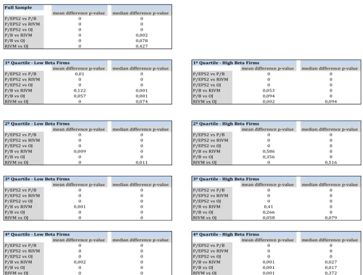
3.4.3 Differences in valuation errors between different valuation models:

In order to test the null hypothesis that the mean and median difference between models is the same, Wilcoxon test was applied once again. This time, the test was only applied for the absolute prediction errors, since the crucial point to test was the magnitude of the error and not the error itself.

Full Sample

mean difference p-value median difference p-value

P/EPS2 vs P/B 0 0 P/EPS2 vs RIVM 0 0 P/EPS2 vs OJ 0 0 P/B vs RIVM 0 0,002 P/B vs OJ 0 0,078 RIVM vs OJ 0 0,427

mean difference p-value median difference p-value mean difference p-value median difference p-value

P/EPS2 vs P/B 0,01 0 P/EPS2 vs P/B 0 0

P/EPS2 vs RIVM 0 0 P/EPS2 vs RIVM 0 0

P/EPS2 vs OJ 0 0 P/EPS2 vs OJ 0 0

P/B vs RIVM 0,122 0,001 P/B vs RIVM 0,053 0

P/B vs OJ 0,057 0,001 P/B vs OJ 0,094 0

RIVM vs OJ 0 0,074 RIVM vs OJ 0,002 0,094

P/EPS2 vs P/B 0 0 P/EPS2 vs P/B 0 0

P/B vs RIVM 0,009 0 P/B vs RIVM 0,586 0

P/B vs OJ 0 0 P/B vs OJ 0,356 0

RIVM vs OJ 0 0,011 RIVM vs OJ 0 0,516

P/B vs RIVM 0,001 0 P/B vs RIVM 0,41 0

P/B vs OJ 0 0 P/B vs OJ 0,266 0

RIVM vs OJ 0 0 RIVM vs OJ 0,058 0,079

P/B vs RIVM 0,002 0 P/B vs RIVM 0,001 0,027

P/B vs OJ 0 0 P/B vs OJ 0,001 0,017

RIVM vs OJ 0 0 RIVM vs OJ 0,001 0,372

1º Quartile - Low Beta Firms

1º Quartile - High Beta Firms

Table 5 – Models valuation performance

Significant levels for the Wilcoxon test comparing the mean and median absolute prediction errors between models are reported for the full sample, for low beta firms, distinguished for different quartiles, and for high beta firms, distinguished for different quartiles.

(36)

29 Analysing carefully table 5, it can it said that the null hypothesis is always rejected when P/EPS2 model is compared with other valuation model. Even so, the same result is not always true when compared the other three models among each others.

Taking these results tested into account for the median comparison between models, the null hypothesis is rejected in almost all the cases excluding the comparison between the RIVM and the OJM model, not only for the full sample data but also for the 2nd_{quartile of leverage level in the high beta firms, since} there cannot be pointed strong and relevant evidences to reject the null hypothesis with only 5% of significance level.

On the other hand, as regards the median differences between models, the situation has shown to be slightly different. In this case, the comparison among P/B, RIVM and OJM is not always rejected, with special attention to the comparison between P/B and RIV models, showing a difference p-value of almost 59%.

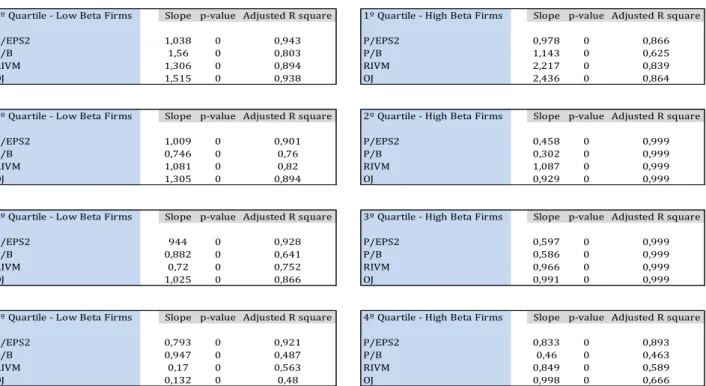
3.4.4 Power of Valuation Models (OLS):

The following test is probably the most important one among the other above analysed in this paper to take factual conclusions concerning the explainability of stock prices in value estimates by each different model.

Taking table 6 into account for analysis, the conclusions we can draw are quite interesting. First of all, in all different scenarios, P/EPS2 ratio is the valuation model that shows the highest unvaried regression, being around a range from 90% to 99%. In this way, and according to these results, this model is the one that best explains the stock prices of companies, notwithstanding their leverage levels or whether they have a low or high beta value. In second place, the valuation model that best explains stock prices is the OJM, followed by RIVM and then P/B model.

(37)

30 In addition to these conclusions drawn, it is also possible to observe that for companies with an extreme leverage level (1st_{and 4}th_{quartile), all models better} explain the stock price of low beta firms than high beta firms. In contrast to this, if we consider average leverage levels, stock prices are best explained for high beta firms.

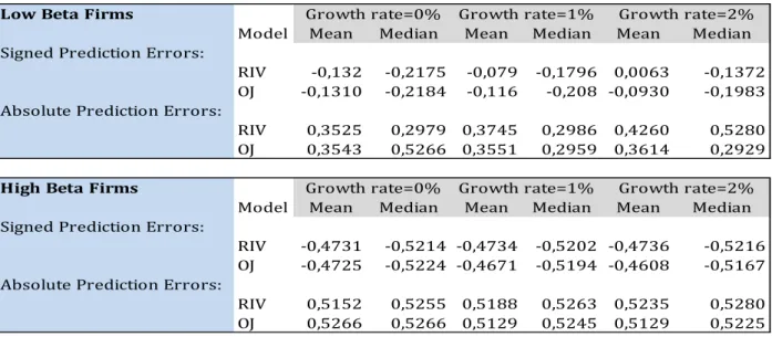
3.4.5 Robustness Test:

As a final test to be discussed in this section, a sensitive analysis was made for the four valuation models. In this case, the variable in question was the growth rate, since this one is considered in studies developed by several theorists as being one of the variables that most influences the empirical outcome.

As it was previously explained, the growth rate is only considered for flow-based models in analysis, i.e. RIV model and OJ model. In the beginning, the growth rate

1º Quartile - Low Beta Firms Slope p-value Adjusted R square 1º Quartile - High Beta Firms Slope p-value Adjusted R square

P/EPS2 1,038 0 0,943 P/EPS2 0,978 0 0,866

P/B 1,56 0 0,803 P/B 1,143 0 0,625

RIVM 1,306 0 0,894 RIVM 2,217 0 0,839

OJ 1,515 0 0,938 OJ 2,436 0 0,864

P/EPS2 1,009 0 0,901 P/EPS2 0,458 0 0,999

P/B 0,746 0 0,76 P/B 0,302 0 0,999

RIVM 1,081 0 0,82 RIVM 1,087 0 0,999

OJ 1,305 0 0,894 OJ 0,929 0 0,999

P/EPS2 944 0 0,928 P/EPS2 0,597 0 0,999

P/B 0,882 0 0,641 P/B 0,586 0 0,999

RIVM 0,72 0 0,752 RIVM 0,966 0 0,999

OJ 1,025 0 0,866 OJ 0,991 0 0,999

P/EPS2 0,793 0 0,921 P/EPS2 0,833 0 0,893

P/B 0,947 0 0,487 P/B 0,46 0 0,463

RIVM 0,17 0 0,563 RIVM 0,849 0 0,589

OJ 0,132 0 0,48 OJ 0,998 0 0,666

Table 6 – Explanatory power of valuation models

Results of estimating the following regression: Pj,F= , where Pj,F is the observed share price of Dividend Paying Firms j; VF,j is the value for security j for the respective models are reported. Regression is estimated for low beta firms, presented for distinguished quartiles, and for high beta firms, presented for distinguished quartiles.

(38)

31 assumed was 2% for the RIV model and 0% for the OJ model. In this case, the growth rate will flow around 0%, 1% and 2%.

As we can see in table 7, the main descriptive statistics, such as, mean and median, suffer a slightly change when the growth rate was altered. Not only the low beta firms but also the high beta firms, the mean and the median signed prediction errors for both models decreases as growth rate increases.

Thus, both valuation models show almost always a slight improvement within signed prediction errors. In contrast, the same descriptive variables of the absolute prediction errors increase as growth rate increases for both valuation models, showing a worsening within absolute prediction errors.

Due to the slightly increased in the absolute prediction errors for both valuation models, the univariate regression will also be altered accordingly.

Looking at table 8, it is easily observable that for both flow-based valuation modes the explanatory power of decreases when the growth rate increases in the all sub samples in analysis.

Low Beta Firms

Model Mean Median Mean Median Mean Median Signed Prediction Errors:

RIV -0,132 -0,2175 -0,079 -0,1796 0,0063 -0,1372 OJ -0,1310 -0,2184 -0,116 -0,208 -0,0930 -0,1983 Absolute Prediction Errors:

RIV 0,3525 0,2979 0,3745 0,2986 0,4260 0,5280 OJ 0,3543 0,5266 0,3551 0,2959 0,3614 0,2929 High Beta Firms

Model Mean Median Mean Median Mean Median Signed Prediction Errors:

RIV -0,4731 -0,5214 -0,4734 -0,5202 -0,4736 -0,5216 OJ -0,4725 -0,5224 -0,4671 -0,5194 -0,4608 -0,5167 Absolute Prediction Errors:

RIV 0,5152 0,5255 0,5188 0,5263 0,5235 0,5280 OJ 0,5266 0,5266 0,5129 0,5245 0,5129 0,5225 Growth rate=0% Growth rate=1% Growth rate=2%

Growth rate=0% Growth rate=1% Growth rate=2%

Signed Prediction Errors (Bias) = (Vj-Pj)/Pj , Absolute Prediction Errors (Accuracy) = |Vj-Pj|/Pj

(39)

32

1º Quartile- Low Beta Firms

Model OLS Coefficient OLS R square OLS Coefficient OLS R square OLS Coefficient OLS R square RIVM 1,5410 0,9190 1,4360 0,9110 1,3060 0,8940

OJ 1,5150 0,9380 1,4150 0,9090 1,2640 0,8500

1º Quartile- High Beta Firms Growth rate=0% Growth rate=1% Growth rate=2%

OJ 2,4360 0,8640 2,4120 0,8630 2,3830 0,8620

2º Quartile- Low Beta Firms Growth rate=0% Growth rate=1% Growth rate=2%

OJ 1,3050 0,8940 1,2930 0,8920 1,2750 0,8890

OJ 0,9290 0,9990 0,9090 0,9990 0,8860 0,9990

OJ 1,0250 0,8660 1,0160 0,8670 0,9990 0,8660

OJ 0,9910 0,9990 0,9870 0,9990 0,9990 0,9820

OJ 0,1320 0,4800 0,1150 0,4660 0,0980 0,4520

OJ 0,9980 0,6660 0,9620 0,6570 0,9220 0,6470

Growth rate=2% Growth rate=0% Growth rate=1%

Table 8 – Explanatory Power of Valuation Models

Results of estimating the following regression: Pj,F= , where Pj,F is the observed share price of Dividend Paying Firms j; VF,j is the value for security j for the respective model are reported for RIVM and OJM when the growth rate is equal to 0%, 1%, and 2%. Regression is estimated for low beta firms, presented for distinguished quartiles, and for high beta firms, presented for distinguished quartiles.