CNN-Based Refinement for Image Segmentation

(1)

F

ACULDADE DE

E

NGENHARIA DA

U

NIVERSIDADE DO

P

ORTO

CNN-Based Refinement

for Image Segmentation

José Soares Rebelo

Mestrado Integrado em Engenharia Informática e Computação Supervisor: Jaime dos Santos Cardoso, PhD

Second Supervisor: Kelwin Fernandes

(2)

c

(3)

CNN-Based Refinement

for Image Segmentation

José Soares Rebelo

Mestrado Integrado em Engenharia Informática e Computação

Approved in oral examination by the committee:

Chair: Alexandre Valle de Carvalho, PhD

External Examiner: Adrian Galdran, PhD Supervisor: Jaime dos Santos Cardoso, PhD

(4)

(5)

Abstract

Image segmentation is the area of computer vision that tries to partition an image into multiple parts, according to some semantic meaning. This is one of the core computer vision problems, and crucial to many applications. Medical imaging is one of such applications that can benefit from automatic image segmentation, due to the large amounts of experience necessary to properly evaluate the images and conditions, and even then facing ambiguity and sometimes leading to disagreement, even between medical professionals.

Traditional image segmentation algorithms operate by iteratively working over an image, as if refining a segmentation until a stopping criterion is met, as the used algorithm determines.

Deep learning is currently playing a crucial role in computer vision, replacing the traditional approaches of feature engineering with learned representations of data. The technology break-throughs in processing power have allowed for the creation of deep neural networks that achieve state-of-the-art performance in many problems, one of them being image segmentation. How-ever, the concept of segmentation refinement is not present anymore, since usually the images are segmented in a single step.

This work focuses on the refinement of image segmentations using deep convolutional neu-ral networks, first by exploring improvements for a method for image segmentation by quality inference. This approach tries to segment an image by first predicting the quality of an existing segmentation and then refining it through gradient descent, by modifying the input segmentation mask while trying to maximize the expected quality. Possible improvements include data aug-mentation, siamese networks, different quality metrics and possible stopping criteria. After that, a network for direct segmentation refinement with an extra quality output is introduced.

We show that data augmentation tuned to the base model and the application of siamese net-works can be used to improve the quality inference performance, despite not improving the seg-mentation refinement process, and that the quality concept can be used as a regularizer while training a network for direct segmentation refinement, achieving better performance results.

(6)

(7)

1 Introduction 1 1.1 Context . . . 1 1.2 Motivation . . . 2 1.3 Goals . . . 2 1.4 Dissertation Structure . . . 3 2 Literature Review 5 2.1 Image Segmentation . . . 5 2.2 Traditional Approaches . . . 5 2.2.1 Thresholding methods . . . 6 2.2.2 Clustering methods . . . 6 2.2.3 Region-based methods . . . 7 2.2.4 Edge-detection methods . . . 7 2.3 Deep Learning . . . 8 2.3.1 Encoder-Decoder Architectures . . . 8 2.3.2 Regularization . . . 10 2.4 Evaluation Metrics . . . 12

2.5 Iterative Segmentation Refinement . . . 14

2.6 Conclusion . . . 14

3 Image Segmentation 17 3.1 Segmentation by Quality Inference . . . 17

3.1.1 Data Augmentation tuned to the base model . . . 21

3.1.2 Stopping Criterion for the Refinement Process . . . 21

3.1.3 Siamese Networks . . . 22

3.1.4 Different Output Metrics . . . 23

3.2 Direct Refinement Networks . . . 23

3.3 Quality Output Extension . . . 24

3.4 Summary . . . 24

4 Implementation and Results 25 4.1 Introduction . . . 25

4.1.1 Datasets . . . 26

4.2 Data Augmentation tuned to the base model . . . 27

4.2.1 Interpolation between masks . . . 27

4.2.2 Training and results . . . 28

4.3 Stopping Criterion for the Refinement Process . . . 30

(8)

CONTENTS

4.4.1 Results . . . 31

4.5 Different/Multiple Output Metrics . . . 32

4.6 Refinement U-Net and Quality Output Extension . . . 34

4.6.1 Results . . . 35 4.7 Summary . . . 36 5 Conclusion 39 5.1 Overview . . . 39 5.2 Contributions . . . 40 5.3 Future Work . . . 40

5.3.1 Direct gradient optimization for backpropagation refinement . . . 40

5.3.2 Fine-tuning for transfer learning . . . 41

5.3.3 Quality-based ensembles . . . 41

5.3.4 Multi-Class Segmentation . . . 41

5.3.5 Weakly supervised learning in sequences of similar images . . . 41

5.3.6 Weakly annotated data . . . 41

5.3.7 Alternative refinement architectures . . . 41

5.3.8 Oracle as stopping criterion for other refinement processes . . . 42

(9)

List of Figures

2.1 SegNet architecture . . . 9

2.2 U-Net architecture . . . 9

2.3 Regularization on a polynomial function fit . . . 11

3.1 Traditional deep learning models / New oracle model . . . 17

3.2 Oracle network: reversed encoder-decoder concept . . . 18

3.3 Oracle network approaches: single stream and dual stream . . . 18

3.4 Oracle network: overview diagram . . . 19

3.5 Oracle network: streams diagram . . . 19

3.6 Oracle network: gossip block . . . 20

3.7 Bad refinement case: predicted and actual dice coefficient . . . 22

3.8 Bad refinement case: segmentation deterioration . . . 22

3.9 Triplet Loss . . . 23

4.1 Datasets - image and segmentation samples . . . 26

4.2 Mask shape interpolation steps . . . 28

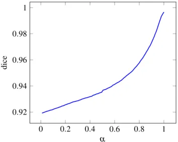
4.3 Dice variation along interpolation between base mask and ground-truth . . . 28

4.4 Siamese Network Implementation . . . 31

4.5 Oracle: Multiple outputs . . . 33

4.6 Hausdorff Distance - Irregular behavior example . . . 34

(10)

(11)

List of Tables

3.1 Original data augmentation transformations . . . 20

4.1 Model hyperparameters . . . 26

4.2 Datasets used and partition sizes . . . 26

4.3 Interpolation for Data Augmentation: Refinement performance results . . . 29

4.4 Interpolation for Data Augmentation: Quality prediction performance results . . 30

4.5 Siamese Network Segmentation: Performance Results . . . 31

4.6 Siamese Network Quality Prediction: Performance Results . . . 32

4.7 Multiple output metrics: refinement performance results . . . 33

4.8 Multiple output metrics quality prediction performance . . . 33

4.9 Refinement U-Net Performance . . . 35

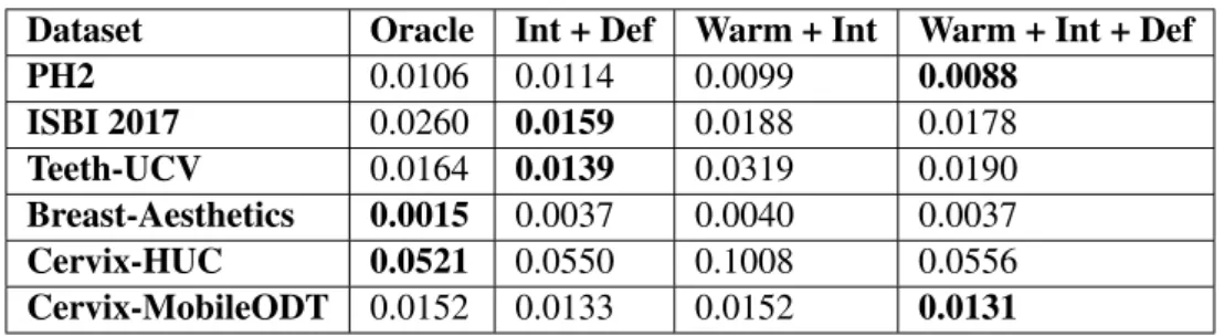
4.10 Refinement U-Net Performance, with quality output and automatic iterations . . . 35

(12)

(13)

Abbreviations

CAD Computer Aided Diagnosis CPU Central Processing Unit CNN Convolutional Neural Network CRF Conditional Random Field

DCNN Deep Convolutional Neural Network FN False Negative

FP False Positive

GPU Graphical Processing Unit MAE Mean Absolute Error MSE Mean Squared Error RNN Recursive Neural Network ROI Region of Interest

TN True Negative TP True Positive

(14)

(15)

Chapter 1

Introduction

Contents 1.1 Context . . . 1 1.2 Motivation . . . 2 1.3 Goals . . . 2 1.4 Dissertation Structure . . . 3

This first chapter gives an overview of the dissertation, by introducing its context, motivation and goals. Finally, it presents the structure of the remaining chapters.

1.1 Context

Image segmentation consists of partitioning an image in multiple parts, without information about what exactly each part represents [48]. However, this expression is normally used when referring to semantic image segmentation, which also tries to partition an image into multiple parts, but those should have some semantic meaning, i.e. belong to one of multiple classes. This represents one of the great challenges for computer vision, since image segmentation is at the base of many computer vision problems.

Traditional image segmentation algorithms, like region-growing methods, usually operate by iteratively working over the image, optimizing some sort of function or performing some operation until a stopping criterion is reached, and the image is considered segmented.

Medical imaging plays a crucial role in the diagnosis and treatment of patients. The medical images are, however, dependent on the visual interpretation of the medical professionals, which is time consuming and prone to error, since some areas require many years of experience in order to properly analyze such medical images. Furthermore, the subjective nature of the interpretation sometimes leads to disagreement, even between experient medical professionals. This motivates the research into Computer Aided Diagnostic (CAD) systems, which should assist the medical professionals and allow for a faster and more accurate diagnosis, as well as reducing the associated costs. At the base of such systems is the image analysis, particularly the semantic segmentation.

(16)

Introduction

1.2 Motivation

In the past years, deep learning has overshadowed traditional algorithms in many areas, by achiev-ing state-of-the-art performance over the old approaches, and sometimes even outperformachiev-ing hu-mans. One of those areas is image segmentation, where deep learning has shown promising re-sults [17].

While deep learning has also been applied to medical image analysis [47], the requirement for huge amounts of data has limited its applications in the field. In the past years some new datasets have been made available, with enough images to allow for the training of deep neural networks.

Deep learning architectures vary, but most apply the same single-step paradigm to image seg-mentation where one image is given to the network as input, and the segseg-mentation is obtained as output. This contrasts with the traditional iterative segmentation methods which needed multiple iterations, usually starting from scratch or from a coarse segmentation and progressing towards a more fine result.

Fernandes et al. [11] have developed a novel segmentation paradigm that tries to segment an image indirectly, by first learning the concept of segmentation quality, and then applying back-propagation over an initial segmentation multiple times in order to iteratively refine it.

1.3 Goals

This research focuses on the study of the architecture presented by Fernandes et al. [11], the iden-tification of some possible improvements, their implementation and testing. This includes the exploration of methodologies such as multitask, transfer learning, siamese networks and regular-ization, as well as research into the possible integration of iterative refinement techniques into deep learning architectures.

The developed and implemented solutions will be evaluated on multiple medical imaging datasets with image segmentation metrics and compared to the base results obtained with the original architecture.

Specifically, the main goals can be elaborated as follows:

1. Research into an alternative data augmentation technique, by introducing segmentations that better prepare the network for the segmentation refinement process.

2. Research into possible stopping criteria for the segmentation refinement process.

3. Research into the application of triplet loss and siamese networks to the quality inference, comparison and segmentation refinement.

4. Research into the usage of different and/or multiple quality metrics for quality inference and segmentation refinement.

5. Research into the direct refinement of a segmentation using an encoder-decoder architecture, possibly extended with a quality output.

(17)

Introduction

1.4 Dissertation Structure

The remainder of this dissertation is structured as follows:

• Chapter 2, “Literature Review” (p. 5), provides a literature review on the areas of image segmentation and deep learning, ending with the main work upon which this dissertation builds.

• Chapter 3, “Image Segmentation” (p. 17), addresses the architecture for segmentation by quality inference at a deeper level, exposing the possible areas of improvement focused by this work, as well as suggested solutions to be explored.

• Chapter 4, “Implementation and Results” (p.25), describes the implementation of the so-lutions proposed in Chapter3, the difficulties faced while executing them and the obtained results.

• Chapter5, “Conclusion” (p.39), concludes this dissertation with an overview of the accom-plished results. Additionally, it includes suggestions for further work.

(18)

(19)

Chapter 2

Literature Review

Contents 2.1 Image Segmentation . . . 5 2.2 Traditional Approaches . . . 5 2.3 Deep Learning . . . 8 2.4 Evaluation Metrics . . . 12

2.5 Iterative Segmentation Refinement . . . 14

2.6 Conclusion . . . 14

This chapter gives an overview into image segmentation, starting with an outline on the clas-sic image segmentation approaches before moving to deep learning and its complementary tech-niques. Finally, it introduces the concept of image segmentation by quality inference, which will be the main base of this dissertation.

2.1 Image Segmentation

Image segmentation consists of classifying each pixel in an image according to its semantic mean-ing. The raw images usually contain some portions that are not relevant to the problem at hand, making it necessary to find the region of interest (ROI), before starting the actual segmentation process.

Each pixel in an image can belong to one of the classes to be considered for segmentation, which can be classified on a broader scale as foreground / background or, on a more fine basis, as each of the more specific classes to be considered for segmentation.

2.2 Traditional Approaches

Traditional image segmentation methods (those which do not use neural networks) make heavy use of domain knowledge in order to properly segment the images, in a process known as feature en-gineering. Feature engineering is a crucial part of many traditional machine learning approaches,

(20)

Literature Review

by using human knowledge and intuition to modify the feature space of the data being analyzed in order to highlight the desired features for further processing [28]. This consists of a lengthy trial and error process that requires large amounts of human involvement and expertise. There is no universally defined method to determine what constitutes a feature, since that is heavily dependent on the problem and type of application.

Depending on what kind of features and how they are being analysed, the traditional ap-proaches for image segmentation can be divided in 4 main techniques [41]: thresholding, clus-tering, region-based and edge-based approaches.

2.2.1 Thresholding methods

Thresholding consists of one of the simplest image segmentation methods, where the pixels are partitioned depending on their intensity value [3]. Thresholding can be further divided into two main types: global and local thresholding.

Global thresholding

Global thresholding uses a single threshold value for the whole image. It can be used only when the pixels from the background and foreground of an image belong to sufficiently distinct distributions. For each pixel f (x, y), the resulting value t(x, y) is decided according to a threshold T .

t(x, y) =    1, if f (x, y) > T 0, if f (x, y) ≤ T (2.1) There are multiple techniques that can be used to determine the threshold. One of the most used ones is Otsu’s method [40]. Otsu’s method determines the the threshold value that optimally separates the two classes, by minimizing their combined spread (intra-class variance).

Local adaptive thresholding

A single threshold will not perform well for many types of images, since most will have uneven illumination. Local thresholding works by applying a different threshold value T (x, y) to each pixel, which depends on the local statistics around it, such as range or variance [39].

t(x, y) =    1, if f (x, y) > T (x, y) 0, otherwise (2.2) 2.2.2 Clustering methods

Clustering algorithms aim to group a set of objects in such a way that objects in the same group (a cluster) show similarities when compared to the remaining objects in the cluster [44]. In image segmentation, the objects to cluster are the pixels belonging to the image to be segmented, and the similarity to be considered is one or more predefined features which depend on the problem being

(21)

Literature Review

tackled. They can range from just using the color of the pixels to more advanced feature vectors that take into consideration extra information from the surrounding area.

The K-means clustering approach aims to partition n observations into k clusters, in which the observations belong to the cluster with the nearest mean [5]. This is an NP-hard problem, but there are some efficient heuristic algorithms that can iteratively converge to a local optimum.

Fuzzy C-means [8] is an adaptation of the K-means algorithm for fuzzy clustering, i.e. each data point can now belong to more than one cluster.

Gaussian mixture models assume that each data point is generated from a mixture of a number of Gaussian distributions with unknown parameters [13]. This can be seen as a generalization of the K-means clustering, by incorporating information about the covariance of the data as well as the centers of the latent Gaussian distributions.

2.2.3 Region-based methods

Region-based methods attempt to determine the segmentation region directly, according to a set of predefined criteria [41]. They can be split into two main types: region growing, and region splitting and merging.

Region growing

In region growing methods, the segmentation regions start from a group of seed pixels, which are iteratively increased by appending to each region neighboring pixels that are similar, according to the defined rules [37]. The region growing stops when no more pixels can be added according to some stopping criterion, like the size or shape of the region, or the non-existence of any more candidate pixels.

The watershed algorithm [49] is based on the simulation of a flooding process. It takes a gray-scale image as input and interprets it as a height map, where the intensity values and the height are directly proportional. The algorithm starts by placing a water source at the regional minimums, and a watershed is found when two bodies of water become connected, marking a segmentation border.

Region splitting and merging

Instead of choosing seed points like the previous approach, region splitting and merging divides the image into a set of unconnected regions and then those regions are merged.

2.2.4 Edge-detection methods

Edges in images consist of groups of pixels that present a rapid transition in intensity, when com-pared to their neighbors. Region boundaries and edges are closely related. There is often a sharp change in intensity at the region boundaries [41] and therefore edge detection techniques have also been used as another segmentation approach.

(22)

Literature Review

Active contour models [27] try to segment images along the edges, while also trying to keep a smooth segmentation border. This is achieved by using an energy function which will be mini-mized.

A deformable spline referred to as snake placed on an image. An energy function is defined, consisting of the sum of the snake’s internal and external energy. The internal energy controls the deformations made to the snake, while the external energy consists of a combination of the forces caused by the image and possible constraints introduced by the user.

Given an initial position for the snake, the energy function is then iteratively optimized, using for example gradient descent.

2.3 Deep Learning

Contrary to the conventional techniques, deep learning allows for the automatic learning of the necessary features for the task at hand, eliminating the manual feature engineering step required before [47]. Its booming usage and success in the last few years can be attributed to the technology advances in processing power, both central processing units (CPUs) and graphical processing units (GPUs), to the availability of large amounts of data and to the advancements in the algorithms.

Deep Convolutional Neural Networks (DCNNs) have demonstrated large success in image-related machine learning tasks. Their training is, however, limited by the amount of training data that is available for their specific task.

In 2009, Jia Deng et al. [26] introduced the ImageNet dataset, which contained 3.2 million in-dividually annotated images. The first big deep learning leap happened in 2012, when Krizhevsky et al. [32] successfully trained a deep convolutional neural network on the ImageNet dataset, win-ning the ImageNet Large Scale Visual Recognition Challenge, achieving an error rate of 15.3%, compared to the 26.2% achieved by the second place candidate. This caused a massive increase in interest and research in the field of deep learning, which has seen many different improvements, techniques and architectures since then.

2.3.1 Encoder-Decoder Architectures

The most used technique for segmentation tasks using deep neural networks consists of encoder-decoder architectures [1]. Encoder-decoder architectures operate in two phases: first, an input image is encoded into a smaller representation, which contains some semantic meaning. On the second step, the image is then decoded into the final segmentation. The encoding step is made of a sequence of convolution and max-pooling layers. The decoding step uses upsampling and convolutions, in a similar symmetric fashion. SegNet [1] was one of the first models to use such an implementation.

Encoder-decoder models have difficulties in avoiding the so-called checkerboard problem caused by the upsampling process. During the encoding step, some information is inevitably lost, which prevents the decoder from producing a refined segmentation, since adjacent pixels in the up-sampled feature map lack relationship information.

(23)

Literature Review

Figure 2.1: SegNet architecture [1]

RefineNet [34] tackles this problem by introducing long-range residual connections to the deeper layers, propagating the earlier captured features, allowing for a higher-resolution segmen-tation.

Pixel Deconvolutional Networks [14] introduce direct relationships between intermediate fea-ture maps, overcoming the checkerboard problem and showing more accurate segmentation re-sults.

Figure 2.2: U-Net architecture [45]

One very successful evolution of the SegNet is the U-Net [45], which won the ISBI cell track-ing challenge 2015, by a large margin. The U-Net uses an encoder-decoder architecture, but before

(24)

Literature Review

each downsampling step in the encoding path, the resulting feature map is concatenated to the cor-responding level in the decoding path, as shown in Figure 2.2. This allows for high resolution features to be combined with the upsampled output, leading to a more precise output avoiding the previously mentioned checkerboard problem.

Outside of the encoder-decoder models, Jegou et al. [25] have achieved state-of-the-art results with a network based on DenseNet [20], which connects each layer to every other layer, in feed-forward fashion.

To improve the DCNNs localization, some modules can be introduced to broaden the context understanding, such as Conditional Random Fields (CRFs) [6], Recurrent layers [51] and Dilated Convolutions [54].

Recurrent layers [51] are composed of 4 RNNs (Recursive Neural Networks) coupled together in a way that captures the local and global spacial structure from the input data. This is done by first sweeping the image vertically with two RNNs (one from bottom to top, the other from top to bottom), using non-overlapping patches. Then, the resulting projections from both RNNs are concatenated, creating a composite feature map which is then swept horizontally by a new pair of RNNs, in the same manner, but without using patches.

Dilated convolutions [54] use the same convolution filter parameters in a dilated form, man-aging to enlarge the receptive field and thus incorporating more context without introducing extra parameters or computation cost.

Besides architectures, there are training techniques that can lead to an easier training of deep neural networks without a large amount of training data. One such technique is transfer learn-ing [53]. Deep neural networks trained on natural images exhibit similar features on the first layers, not tied to a specific dataset, like edge detectors. This makes it possible to train a network first on a large dataset such as ImageNet, and then locking the first layers, training just the next ones on the desired dataset.

Iglovikov and Shvets [22] have shown that using the weights from a VGG11 network pre-trained on the ImageNet dataset as the encoding path of a U-Net leads to better results even with a small training dataset, having won the Kaggle’s “Carvana Image Masking Challenge”.

2.3.2 Regularization

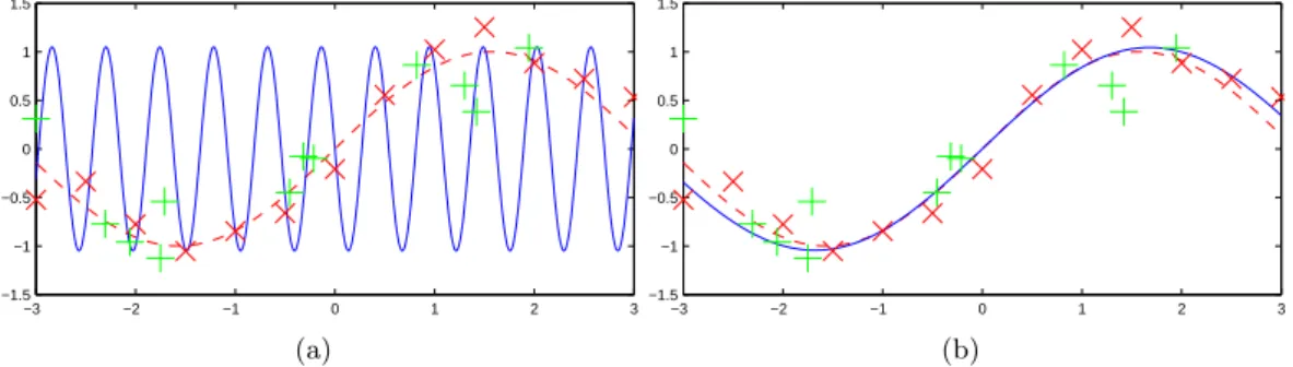
Regularization is a key strategy to avoid overfitting [15]. Overfitting occurs when the network starts to learn the actual training data and possibly the noise associated with it, instead of the fea-tures that lead to the expected output, and thus failing to generalize for new examples. One of the simplest examples can be seen when trying to fit a polynomial curve to sampled data (see Fig-ure2.3). With the right fit, the curve will miss some points but it will be smooth and close enough to the original function. When it overfits, it will display an erratic behavior and be completely off, despite fitting almost perfectly to the training samples. In neural networks, overfitting occurs when the training error is still decreasing, but the validation error starts getting worse, indicating that the network is losing the capacity to generalize.

(25)

Literature Review Supervised Learning X , C p(x, c) U (c, f (x|θ)) − λP (θ) θ c∗_{= f(x}∗_|θ)

x∗ _{Figure 13.4: Empirical risk approach. Given}

the dataset X , C, a model of the data p(x, c) is made, usually using the empirical distribu-tion. For a classifier f(x|θ), the parameter θ is learned by maximising the penalised empir-ical utility (or minimising empirempir-ical risk) with respect to θ. The penalty parameter λ is set by validation. A novel input x∗_{is then assigned to}

class f(x∗_{|θ), given this optimal θ.}

−3 −2 −1 0 1 2 3 −1.5 −1 −0.5 0 0.5 1 1.5 (a) −3 −2 −1 0 1 2 3 −1.5 −1 −0.5 0 0.5 1 1.5 (b)

Figure 13.5: (a): The unregularised fit (λ = 0) to training given by ×. Whilst the training data is well fitted, the error on the validation examples, + is high. (b): The regularised fit (λ = 0.5). Whilst the train error is high, the validation error (which is all important) is low. The true function which generated this noisy data is the dashed line; the function learned from the data is given by the solid line.

Drawbacks of the empirical risk approach

• It seems extreme to assume that the data follows the empirical distribution, particularly for small amounts of training data. To generalise well, we need to make sensible assumptions as to p(x) – that is the distribution for all x that could arise.

• If the utility (or loss) function changes, the discriminant function needs to be retrained.

• Some problems require an estimate of the confidence of the prediction. Whilst there may be heuristic ways to evaluating confidence in the prediction, this is not inherent in the framework.

• When there are multiple penalty parameters, performing cross validation in a discretised grid of the parameters becomes infeasible.

• It seems a shame to discard all those trained models in cross-validation – can’t they be combined in some manner and used to make a better predictor?

Example 60 (Finding a good regularisation parameter). In fig(13.5), we fit the function a sin(wx) to data, learning the parameters a and w. The unregularised solution fig(13.5a) badly overfits the data, and has a high validation error. To encourage a smoother solution, a regularisation term Ereg = w2 is used.

The validation error based on several different values of the regularisation parameter λ was computed, finding that λ = 0.5 gave a low validation error. The resulting fit to novel data, fig(13.5b) is reasonable.

13.2.4 Bayesian decision approach

An alternative to using the empirical distribution is to fit a model p(c, x|θ) to the train data D. Given this model, the decision function c(x) is automatically determined from the maximal expected utility (or

258 DRAFT March 9, 2010

Figure 2.3: Regularization on a polynomial function fit. Training samples in red, validation ex-amples in green, original function represented by the red dashed line. (a) The unregularized fit. (b) The regularized fit [2]

L1 and L2 regularization are the most common types of regularization. These penalize very large weights by including them as a regularization term in the cost function that is being opti-mized. Smaller weights lead to simpler models, which reduces overfitting.

L1 Regularization

In L1 regularization, the weights affect the cost function linearly with the sum of their absolute values, scaled by a factor of λ , that scales the regularization strength.

CostFunction= Loss + λ ×

_∑

|w| (2.3)

L2 Regularization

In L2 regularization, the weights affect the cost function quadratically with the sum of their squared values, also scaled by a factor of λ .

CostFunction= Loss + λ ×

_∑

w2 (2.4)

Weight Decay [16] acts directly on the weight updates, multiplying them by a factor slightly smaller than 1, preventing them from growing too large. This is equivalent to L2 Regularization for stochastic gradient descent if the weight decay factor if reparametrized based on the learning rate, but not for adaptative gradient algorithms such as Adam [36].

Another cause of overfitting is the co-adaptation between neurons on the training data. This consists of some network units relying on others to extract certain features, while the desire is for each unit to extract the necessary features by itself.

Dropout [19] is another regularization technique that prevents co-adaptations by randomly disabling units throughout the network. This effectively causes a drop in the network capacity, forcing it to learn multiple models at the same time and averaging them.

(26)

Literature Review

DropConnect [52] acts in a similar way, but instead of fully disabling a unit it just disables some of the connections to it. DropConnect is a basically generalization of Dropout, since it can lead to even more models, in addition to the ones that Dropout already makes possible.

Stochastic depth [21] drops entire layers, bypassing them with identity functions, and this way managing to train very deep networks beyond 1200 layers, while still getting improvements in test error.

Early-stopping [15] is one type of cross-validation strategy, where the network training is stopped when the performance on a validation set stops improving. Then, the obtained network is tested on a third set called the test set, to verify that no overfitting occurred on the validation set.

Batch Normalization [24] makes normalization a direct part of the network, by performing it for each training batch between layers. This is useful because as the parameters of the previous layer change, its output distribution is now different, which can saturate the non-linearities in the current layer. Using batch normalization stabilizes the network, allowing for higher learning rates and decreasing the importance of optimal weight initialization.

Most of the described regularization techniques work explicitly, by reducing the effective ca-pacity of the network [18]. Data augmentation [42], on the other hand, has proved to be effective at improving the generalization performance of a network by introducing artificial modifications in the existing training samples, like rotations, crops, flips and deformations in the case of images. Since the network itself is not changed, its capacity remains unchanged. It has been shown that data augmentation alone can achieve the same performance or higher when compared to models trained with other regularization techniques [18], especially when facing small datasets.

2.4 Evaluation Metrics

Although the results can be visually analyzed, in order to objectively evaluate and compare the per-formance of any segmentation algorithm or variation in parameters, some metrics must be chosen. Fenster and Chiu [9] define and review 3 types of metrics: accuracy, precision and efficiency.

The accuracy of a segmentation determines how close it is to a reference segmentation, which can be the ground-truth or a segmentation determined by an expert in the field that is being studied. These terms are normally used interchangeably.

For each class, each segmented pixel can be then be seen as a True Positive (TP), True Neg-ative (TN), False Positive (FP) or False NegNeg-ative (FN). TP and TN represent the pixels that were correctly classified as belonging or not to the class, respectively. Similarly, FP and FN represent the pixels that were misclassified as belonging or not to that class, respectively.

(27)

Literature Review

Sensitivity

Sensitivity or Recall, determines the true positive fraction, that is, the fraction of pixels that were correctly classified as belonging to the class.

Sensitivity= |TP|

|TP| + |FN| (2.5)

Specificity

Specificity determines the the fraction of pixels that were correctly classified as not belonging to the class.

Speci f icity= |TN|

|TN| + |FP| (2.6)

Accuracy

Accuracy determines the fraction of pixels that were correctly classified. Accuracy= |TP| + |TN|

|TP| + |TN| + |FP| + |FN| (2.7)

Dice Similarity Coefficient

Dice Similarity Coefficient, also known as F1 score, is the most used metric in medical segmenta-tion. It determines the overlap ratio between the reference and the obtained segmentasegmenta-tion.

DSC = 2 × |TP|

2 × |TP| + |FP| + |FN| (2.8)

Jaccard Index

Jaccard Index determines the intersection over union between the reference and the obtained seg-mentation.

JAC = |TP|

|TP| + |FP| + |FN| (2.9)

The Jaccard Index is related to the Dice Similarity Coefficient, both being within a factor of 2 from each other:

DSC =2 × JAC

1 + JAC (2.10)

The metrics were described in a binary classification setting (either the pixel belongs to a class or not). However, they can be used in multi-class classification via micro or macro averaging [35], where the results are averaged using all the classes to produce one final result.

Sometimes, comparing the segmented areas directly alone doesn’t describe the performance accurately. Kim and Huang [29] use the Jaccard index, combined with both the Euclidean distance between the centroids of the ground truth and the obtained area and with the aspect ratio of both areas.

(28)

Literature Review

Choosing the proper evaluation metric for the problem at hand is also important, since metrics can have a bias towards/against some properties. Taha et al. [50] devise a method for ranking metrics according to their overall bias.

In many medical imaging applications there is the problem of class imbalance, which occurs when the training data contains many more examples for one class than for the others, making it so that the network becomes biased towards predicting that class [17]. This can be especially problematic for medical applications, since the class with fewer examples usually corresponds to lesions, for example, which will make the network report a lot of false positives. Hashemi et al. [17] developed an asymmetric loss function to mitigate this issue, achieving state-of-the-art results.

2.5 Iterative Segmentation Refinement

There is already some existing work on applying deep learning to the problem of iterative segmen-tation refinement.

Kim et al. [30] use an encoder-decoder network similar to the U-Net, augmented with an extra input for an already existing segmentation. The existing segmentation is subjected to convolutional layers, before concatenating the obtained feature maps with the ones from the image. A new objective function based on the Dice coefficient is also proposed, which captures the improvement in Dice coefficient between iterations.

Lessmann et al. [33] use CNNs to iteratively segment images of vertebrae. By processing the image in patches from top to bottom, the network retains information about the already segmented vertebrae and uses it to find and segment the next not yet segmented vertebra.

Segmentation methods usually work directly on obtaining output segmentation. Fernandes et al. [11] present a network that infers the quality of a segmentation given an image and seg-mentation pair. The segseg-mentation quality consists of some evaluation metric like those described in Section2.4(dice coefficient in the original work). This allows for data augmentation through the unsupervised generation of synthetic segmentations for an image, given that the segmentation quality for the objective function can be easily determined, having the ground-truth before being augmented.

With the trained model, it is then possible to iteratively refine a segmentation through back-propagation on the input segmentation, towards a local maximum for the quality.

This architecture will be the used as a base for the dissertation, and will be described further in Section3.1.

2.6 Conclusion

The area of image segmentation is an ever-evolving and very challenging field, showing the need for the combination of multiple techniques in a pipeline to tackle it successfully, from image pre-processing and feature analysis to the segmentation refinement. Traditional methods work, but

(29)

Literature Review

need to be fine-tuned for specific situations, and in some fields they lack objective evaluation. Deep learning is promising, but currently faces problems with the lack of training data, especially in the medical field.

There is some existing work into segmentation refinement using deep convolutional neural networks, with promising results. Usually the quality concept is optimized while training segmen-tation networks, but never directly in the network itself. The quality inference notion and subse-quent application to image segmentation introduces a new concept that shows a lot of potential, albeit with some drawbacks and areas for improvement that will be the focus of this dissertation.

(30)

(31)

Chapter 3

Image Segmentation

Contents

3.1 Segmentation by Quality Inference . . . 17

3.2 Direct Refinement Networks . . . 23

3.3 Quality Output Extension . . . 24

3.4 Summary . . . 24

This chapter presents the architecture for image segmentation by quality inference at a deeper level, some problems and possible improvements that will be explored during this dissertation.

3.1 Segmentation by Quality Inference

Briefly introduced in Chapter2, the technique proposed by Fernandes et al. [11] uses a deep net-work that predicts the segmentation quality, allowing for the iterative refinement of a segmentation using backpropagation. The model that originates from this architecture will be referred to from now on as oracle.

Traditional deep learning segmentation techniques work directly on learning a model, depicted in Figure3.1awhich, given an image, predicts the desired segmentation by optimizing some metric of quality. Both the input and output spaces are multidimensional, giving rise to the necessity of strong techniques for data augmentation in order to facilitate learning.

Model Mask Image (a) Traditional Model Image Quality Mask (b) Oracle Figure 3.1: Traditional deep learning models / New oracle model

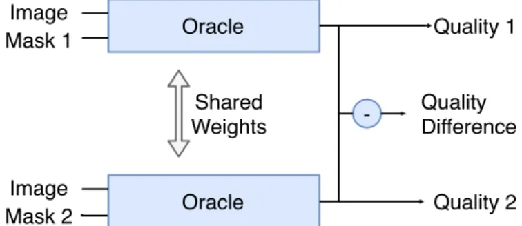
In this oracle architecture, the input consists of an image and mask pair, and the output is now a single number (see Figure3.1b).

Conceptually, one possible interpretation consists of reversing the decoder from an encoder-decoder network, turning the segmentation output into an input and using both inputs to learn a

(32)

Image Segmentation

proxy function, now using the old latent dimension as a quality output, as illustrated in Figure3.2. The inference process for the segmentation refinement can then be achieved through iterative backpropagation on the input mask, maximizing the expected quality, with an associated step size in order to avoid large segmentation changes through large gradients.

Image Mask

Quality

Figure 3.2: Oracle network: reversed encoder-decoder concept

The oracle implementation can be done in one of two ways:

(a) concatenating the mask to the image as an additional channel and using a traditional CNN (see Figure3.3a)

(b) having two separate streams, one for the input image and other for the segmentation mask and then concatenating their latent representation (see Figure3.3b)

⊕ _CNN Quality

Fig. 3: Diagram representing a potential single-mixed stream approach to the problem.

CNN

⊕ Quality

Fig. 4: Diagram representing a potential dual stream approach to the problem.

regularized loss function

min

θ

X

k

Lθ(f (ik, mk), qk) + λR(θ), (1)

where L can be instantiated to the squared error of the estimated quality and the corresponding ground-truth quality and R is a regularizer of the model complexity (e.g. L2).

In this approach, we assume that, during training, a quality function for each image-mask pair is available.

The most straightforward strategy to solve this problem would be to use a traditional Convolutional Neural Net-work (CNN) where the mask is appended to the image as an additional channel (see Fig. 3). These two data sources (i.e. image and mask) belong to different categories (real-valued and binary) but are handled by the same operation (i.e. convolution) which may difficult the learning process.

An alternative approach would be to have separate streams for the input image and masks (see Fig. 4), being merged in the final dense blocks by concatenating their latent representation. The main drawback of this model would be that as we move deeper through the network, the intrinsic loss of resolution would limit the analysis of low-level patterns. Moreover, since each stream works with a different type of data, it is not clear how similar would be their latent representation.

In this work, we propose a deep architecture to tackle this problem, allowing an early integration of the information from image and masks. The main intuition behind this architecture is (i) having two streams that attempt to model the regions defined as foreground and background respectively by the input mask; (ii) streams communicate – “gossips” – to each other in order to increase/decrease their confidence on the recognition of their corresponding regions. In the rest of this section, we formalize the proposed architecture and its training

Mask Input 1-Mask Stream Stream dense dense ... ... dense dense ⊕ dense ... dense Quality

Fig. 5: Diagram of the general Gossip network.

M1 I1 I2 M2 con v con v gossip gossip con v con v gossip gossip pooling pooling pooling pooling I1 I2 M1 M2

Fig. 6: Diagram of the two streams containing the gossip blocks. Ft Ft Fo Fo Io Mt It con v con v Ft Fo × × − i − _Fˆ_t Gossip block

Fig. 7: Diagram of the gossip block. Thick arrows define the first argument of the operations that are not commutative. (a) Single stream

⊕ _CNN Quality

CNN

⊕ Quality

regularized loss function

min

θ

X

k

Lθ(f (ik, mk), qk) + λR(θ), (1)

In this work, we propose a deep architecture to tackle this problem, allowing an early integration of the information from image and masks. The main intuition behind this architecture is (i) having two streams that attempt to model the regions defined as foreground and background respectively by the input mask; (ii) streams communicate – “gossips” – to each other in order to increase/decrease their confidence on the recognition of their corresponding regions. In the rest of this section, we formalize the proposed architecture and its training procedure. Mask Input 1-Mask Stream Stream dense dense ... ... dense dense ⊕ dense ... dense Quality

Fig. 7: Diagram of the gossip block. Thick arrows define the first argument of the operations that are not commutative. (b) Dual stream

Figure 3.3: Oracle network approaches: (a) single stream, (b) dual stream [11] 18

(33)

Image Segmentation

Both approaches have some drawbacks, because the images and segmentation masks belong to different categories (the image consists of real values, while the mask is binary), which in (a) may difficult learning while being handled by the same operation (convolution) and in (b) may result in very different latent representations.

⊕ _CNN Quality

CNN

⊕ Quality

regularized loss function min

θ

X

k

Lθ(f (ik, mk), qk) + λR(θ), (1)

In this work, we propose a deep architecture to tackle this problem, allowing an early integration of the information from image and masks. The main intuition behind this architecture is (i) having two streams that attempt to model the regions defined as foreground and background respectively by the input mask; (ii) streams communicate – “gossips” – to each other in order to increase/decrease their confidence on the recognition of their corresponding regions. In the rest of this section, we formalize the proposed architecture and its training procedure. Mask Input 1-Mask Stream Stream dense dense ... ... dense dense ⊕ dense ... dense Quality

Fig. 7: Diagram of the gossip block. Thick arrows define the first argument of the operations that are not commutative.

Figure 3.4: Oracle network: overview diagram [11]

This problem is tackled in the original work by having two streams that attempt to model the categories represented by the mask (one for the background, other for the foreground). The streams then communicate (“gossip”) between each other, increasing/decreasing their confidence in the classification of each pixel. The gossip streams are followed by dense layers, with the final quality score as output. The full network architecture is shown in Figure3.4.

⊕

_CNN

Quality

Fig. 3: Diagram representing a potential single-mixed stream

approach to the problem.

CNN

⊕

Quality

Fig. 4: Diagram representing a potential dual stream approach

to the problem.

regularized loss function

) + λR(θ),

(1)

where L can be instantiated to the squared error of the

estimated quality and the corresponding ground-truth quality

and R is a regularizer of the model complexity (e.g. L

2

).

In this approach, we assume that, during training, a quality

function for each image-mask pair is available.

The most straightforward strategy to solve this problem

would be to use a traditional Convolutional Neural

Net-work (CNN) where the mask is appended to the image as

an additional channel (see Fig. 3). These two data sources

(i.e. image and mask) belong to different categories

(real-valued and binary) but are handled by the same operation (i.e.

convolution) which may difficult the learning process.

An alternative approach would be to have separate streams

for the input image and masks (see Fig. 4), being merged in the

final dense blocks by concatenating their latent representation.

The main drawback of this model would be that as we move

deeper through the network, the intrinsic loss of resolution

would limit the analysis of low-level patterns. Moreover, since

each stream works with a different type of data, it is not clear

how similar would be their latent representation.

In this work, we propose a deep architecture to tackle this

problem, allowing an early integration of the information from

image and masks. The main intuition behind this architecture

is (i) having two streams that attempt to model the regions

defined as foreground and background respectively by the

input mask; (ii) streams communicate – “gossips” – to each

other in order to increase/decrease their confidence on the

recognition of their corresponding regions. In the rest of this

section, we formalize the proposed architecture and its training

Mask

Input

1-Mask

Stream

dense

...

dense

⊕

dense

...

dense

Quality

Fig. 5: Diagram of the general Gossip network.

M

1

I

₁

I

2

M

₂

con

v

con

v

gossip

con

v

con

v

gossip

pooling

I

₁

×

−

i

−

_F

ˆ

_t

Gossip block

Fig. 7: Diagram of the gossip block. Thick arrows define the

first argument of the operations that are not commutative.

Figure 3.5: Oracle network: streams diagram [11]

Each stream receives as input the image being segmented and its corresponding foreground or background mask (which corresponds to the inverted foreground mask, in binary classification). Each stream, shown in more detail in Figure3.5, is made up of alternating convolutional and gossip blocks, with pooling applied at the end of the stream to both the obtained feature maps and

(34)

Image Segmentation

segmentation masks. This provides interaction between the streams at each level of resolution, allowing for an early reinforcement or penalization of the respective classification. At the end of a stream, average pooling was used.

⊕

_CNN

Quality

Fig. 3: Diagram representing a potential single-mixed stream

approach to the problem.

CNN

⊕

Quality

Fig. 4: Diagram representing a potential dual stream approach

to the problem.

regularized loss function

) + λR(θ),

(1)

where L can be instantiated to the squared error of the

estimated quality and the corresponding ground-truth quality

and R is a regularizer of the model complexity (e.g. L

2

).

In this approach, we assume that, during training, a quality

function for each image-mask pair is available.

The most straightforward strategy to solve this problem

would be to use a traditional Convolutional Neural

Net-work (CNN) where the mask is appended to the image as

an additional channel (see Fig. 3). These two data sources

(i.e. image and mask) belong to different categories

(real-valued and binary) but are handled by the same operation (i.e.

convolution) which may difficult the learning process.

An alternative approach would be to have separate streams

for the input image and masks (see Fig. 4), being merged in the

final dense blocks by concatenating their latent representation.

The main drawback of this model would be that as we move

deeper through the network, the intrinsic loss of resolution

would limit the analysis of low-level patterns. Moreover, since

each stream works with a different type of data, it is not clear

how similar would be their latent representation.

In this work, we propose a deep architecture to tackle this

problem, allowing an early integration of the information from

image and masks. The main intuition behind this architecture

is (i) having two streams that attempt to model the regions

defined as foreground and background respectively by the

input mask; (ii) streams communicate – “gossips” – to each

other in order to increase/decrease their confidence on the

recognition of their corresponding regions. In the rest of this

section, we formalize the proposed architecture and its training

procedure.

Mask

Input

1-Mask

Stream

dense

...

dense

⊕

dense

...

dense

Quality

Fig. 5: Diagram of the general Gossip network.

M

1

I

1

I

2

M

2

con

v

con

v

gossip

con

v

con

v

gossip

pooling

I

1

×

−

i

−

_F

ˆ

_t

Gossip block

Fig. 7: Diagram of the gossip block. Thick arrows define the

first argument of the operations that are not commutative.

Figure 3.6: Oracle network: gossip block. Bold arrows indicate the first argument of the operation, which are not commutative [11]

The gossip blocks, shown in detail in Figure3.6, receive as input the feature map from the previous corresponding convolutions on both streams and its own stream’s segmentation mask. Then, the stream activations are penalized, if they have a stronger value in the opposite stream.

Contrary to the traditional encoder-decoder networks, where the same data augmentation trans-formations have to always be applied in parallel to both the image and the segmentation mask, this new technique allows for different transformations to be applied to the image and mask, since the output quality can then be calculated with the ground truth, incrementing the available training data further than it was possible before. This should allow the network to learn the impact of each type of error in a segmentation’s quality, and opens up the possibility to the usage of a large num-ber of data augmentation transformations. The default data augmentation transformations used by the reference work are enumerated in Table3.1with the respective parameters.

Table 3.1: Original data augmentation transformations, and the variable parameters for each trans-formation.

Transformation Parameters

Elastic deformations α , θ , α0 Morphological (erosion and dilation) size Random pixel switches # pixels

Rotations angle

Flip transformations horizontal and/or vertical

(35)

Image Segmentation

In order to provide the network with a balanced range of dice coefficient values, the impact of each parameter on the dice coefficient was determined empirically. For each transformation, the parameters were drawn using grid-search, and the dice-coefficient between the ground-truth and augmented masks was calculated and discretized into B bins (B = 8 in the original work). Stochastic transformations (elastic deformations and random pixel switches) were repeated 10 times, for each ground-truth mask. With that distribution determined, a second distribution was computed, from which parameters could be sampled while ensuring a uniform distribution of the dice coefficient across all bins.

Given an image and mask pair, the refinement process can be seen as “walking” through the solution space, by adding / removing parts of the segmentation while trying to maximize the predicted quality. This is done in practice using backpropagation over the mask, maximizing the predicted quality.

With this in mind, there are some techniques and modifications that could improve both the quality prediction and the subsequent iterative segmentation process, which will be presented in the following sections, along with some difficulties that were identified and the investigation into possible solutions.

3.1.1 Data Augmentation tuned to the base model

In the reference work, the network is trained with generic data augmentation techniques. While this covers a very wide range of transformations and gives good results for the quality prediction process, it might benefit from a more tuned data augmentation process, more directed to the final goal of segmentation refinement.

The default data augmentation produces results that, while relevant in the training for the qual-ity evaluation, are not representative of the inputs the network will usually try to refine, obtained from the base models.

With this in mind, the network should be trained with segmentation inputs that better illustrate the refinement process, i.e. the masks that are seen throughout the segmentation space between the output from the base models and the ground truth, in order to better prepare it for the corrections necessary in order to properly refine the segmentations.

3.1.2 Stopping Criterion for the Refinement Process

One problem of any refinement process that doesn’t have a clear finished state is determining the stopping criterion, that is one which doesn’t stop too early but also doesn’t continue when the segmentation is possibly getting worse. This is especially problematic for the latter situation, since the network will always try to improve a segmentation, even when that “improvement” is actually destructive. Furthermore, since we are actually using backpropagation over the mask, the network will not be able to correctly predict the performance of its own refinement since, by definition, when trying to refine the segmentation by optimizing the quality, every step it takes will improve its own perception of the segmentation quality, even when it declines (assuming the step size is

(36)

Image Segmentation

small enough not to go directly to a lower quality value). One such case is illustrated in Figure3.7 and Figure3.8. They show one extreme case where the image is hard to segment and the network quality prediction actually has a large error. For every refinement step, the network’s predicted quality increases, while the actual quality is deteriorating. As seen in Figure3.8, in this case the network started opening holes in the area that should actually be segmented.

0 5 10 15 20 25 0.6 0.7 0.8 0.9 1 iteration dice Actual Predicted

Figure 3.7: Bad refinement case: predicted and actual dice coefficient

(a) Image (b) Ground truth (c) Base (d) Refined

Figure 3.8: Bad refinement case: segmentation deterioration. The segmentation was refined for 11 iterations.

It is then necessary to try to find another stopping criterion that doesn’t fully rely on the actual value of the predicted quality. This could involve the actual variation rate of the predicted quality or other metrics such as the foreground/background ratio and their variation along the refinement process.

3.1.3 Siamese Networks

Predicting the quality of a segmentation is not an easy task, especially in certain domains with more difficult boundaries and thus ambiguity on the fine details of the segmentation. Siamese Networks could be used to try to improve this distinction between segmentations of the same

(37)

Image Segmentation

image, giving the network not only one but two different segmentations per image, and thus trying to also learn directly what makes one segmentation better over another.

This quality comparison idea is inspired by the Triplet Loss [46], where a network learns to distinguish faces using 3 examples: an anchor, a positive example and a negative example (see Figure3.9). The network then tries to minimize the distance between the anchor and the positive example (because they are from the same person) and maximize the distance between the anchor and negative example (they belong to different persons).

In the case of quality prediction, the image that is being segmented is used as an anchor of sorts, while the network must learn the concept of image quality, while at the same time reinforcing the differences between two given segmentations of different qualities.

Figure 3.9: Triplet Loss [46]

3.1.4 Different Output Metrics

While the dice coefficient works for evaluating the actual overlapping areas from the reference segmentation and the output of a network, it treats every pixel in the same way, giving the network no way to easily discern areas of more importance for the segmentation. It might focus on the easier areas which provide a boost in the dice coefficient, not paying much attention to the details that would improve it further. There are metrics that might better capture different segmentation quality semantics other than the overlapping area, like the distance between the segmentations’ borders.

3.1.4.1 Multiple Output Metrics

Since different metrics evaluate different segmentation concepts, after having identified other met-rics a network that predicts multiple metmet-rics for the same image pair could also be achieved, which theoretically could then use the concepts represented from each metric to refine a given segmen-tation, combining them into a more comprehensive concept of segmentation quality.

3.2 Direct Refinement Networks

As mentioned in Section 2.3, most of the state-of-the-art deep segmentation architectures use encoder-decoder architectures, which face some resolution and context loss during the encoding

(38)

Image Segmentation

process. Similarly, when attempting to segment an image, the network will give the same impor-tance to any area on the entire image, making it harder for it to discern some parts that might be more important for later segmentation.

By giving the network some extra information before the encoding step in the form of a pre-vious attempted segmentation by another network, the encoder can now learn how to use that information to focus more thoroughly on certain areas of the image that are believed to be close to the segmentation, thus refining the provided mask into a better one.

3.3 Quality Output Extension

A refinement network could also be extended with a quality output, calculated by evaluating the network’s latent dimension after the encoding step, outputting the quality of the segmentation before the refinement step. By training the network with this quality output, it would be forced to not only learn how to improve a given segmentation but also its quality, which would indicate how far the input segmentation is from the desired ground-truth.

The quality output can also be used to evaluate the segmentation quality, allowing for the iterative process to continue until the quality stops improving. This time, however, we should not face the same difficulties presented in Section3.1.2. Since there is no backpropagation involved, the network should now more easily identify a quality decrease from a bad iteration step and stop the segmentation refinement. While this is actually arguable, since it would not be a problem in the first case if the network had learned the quality perfectly, training a perfect network is not feasible for many tasks. With that in mind, it is not safe to rely fully on backpropagation using an imperfect network, with no other stopping criterion.

3.4 Summary

Segmentation quality prediction can be used to iteratively refine a mask through backpropagation, by maximizing the expected quality.

This new technique has some possible enhancements that might improve the obtained results, such as extended data augmentation through the introduction of segmentations that further illus-trate the refinement process, siamese networks for quality comparison and different output metrics that capture other segmentation semantics. The stopping criterion for the refinement process is still an open problem with no clear solution, given the limitations faced by the quality prediction when using backpropagation, which does not allow for the predicted quality to decline, even when it does in reality.

Encoder-decoder architectures can be extended with an extra channel for segmentation refine-ment and a quality output extension, which should allow for the simultaneous direct segrefine-mentation refinement and quality prediction.

(39)

Chapter 4

Implementation and Results

Contents

4.1 Introduction . . . 25

4.2 Data Augmentation tuned to the base model . . . 27

4.3 Stopping Criterion for the Refinement Process . . . 30

4.4 Siamese Network . . . 30

4.5 Different/Multiple Output Metrics . . . 32

4.6 Refinement U-Net and Quality Output Extension . . . 34

4.7 Summary . . . 36

This chapter presents the implementation details for the improvements proposed in the previ-ous chapter, as well as the performance results obtained.

4.1 Introduction

All of the solutions described in this chapter were implemented in Keras, using TensorFlow as the backend, given the fast prototyping provided by Keras with its high level APIs, the author’s famil-iarity with TensorFlow, its high performance, good documentation and support, and the already existing code-base and trained models from the reference work [11].

In order to allow reproducible results, the dataset partitions and random seeds are fixed. The base models used are the same as the ones used in the reference work.

All the images are directly used in RGB format, with all the color components normalized to the [0, 1] range. There is minimal preprocessing applied, being just resized to 128 × 128 to conform to the original work and allow for faster training and the need for lower computational resources.

For the masks, a binary setting is considered, where pixel values of 0 indicate background and pixel values of 1 indicate foreground (the subject of interest being segmented on each dataset).

The training is done for up to a maximum of 500 epochs or 50 epochs without improvement on the validation set, in order to avoid overfitting.

(40)

Implementation and Results

Unless otherwise stated, the hyperparameter configuration for the models is the one described in Table4.1, determined to have the best performance using cross-validation. Adam [31] was used as the algorithm for gradient optimization, with a learning rate of 1e−4.

All the dice coefficient values in the results have been multiplied by 100, being in the form of a percentage, for easier readability.

Table 4.1: Model hyperparameters

Hyperparameter Value

# Convolution Levels 4 # Consecutive Convolutions 2 # Convolution Filters 32 Convolution Filter Size 3

# Dense Levels 1

Dense Stream Width 512 L2 regularization 0.001 Convolution Activation ReLU

4.1.1 Datasets

For the training and evaluation of the proposed solutions, the datasets summarized in Table 4.2 were used. Some examples from each dataset are displayed in Figure4.1

Table 4.2: Datasets used and partition sizes

Dataset # images # train # test # validation

PH2 [38] 200 120 40 40 ISBI 2017 [7] 2750 2000 600 150 Teeth-UCV [12] 100 60 20 20 Breast-Aesthetics [4] 120 72 24 24 Cervix-HUC [10] 287 171 58 58 Cervix-MobileODT [23] 1613 940 338 335

PH2 ISBI 2017 Teeth-UCV Breast HUC MobileODT