REM WORKING PAPER SERIES
Static versus Dynamic Deferred Acceptance in School Choice:
Theory and Experiment
Flip Klijn, Joana Pais, Marc Vorsatz
REM Working Paper 004-2017
September 2017
REM – Research in Economics and Mathematics
Rua Miguel Lúpi 20,1249-078 Lisboa, Portugal
ISSN 2184-108X
Any opinions expressed are those of the authors and not those of REM. Short, up to two paragraphs can be cited provided that full credit is given to the authors.
Static versus Dynamic Deferred Acceptance
in School Choice: Theory and Experiment
Flip Klijn
∗Joana Pais
†Marc Vorsatz
‡November 22, 2016
Abstract
In the context of school choice, we experimentally study how behavior and outcomes are affected when, instead of submitting rankings in the student proposing or receiving deferred acceptance (DA) mechanism, participants make decisions dynamically, going through the steps of the underlying algorithms. Our main results show that, contrary to theory, (a) in the dynamic student proposing DA mechanism, participants propose to schools respecting the order of their true preferences slightly more often than in its static version while, (b) in the dynamic student receiving DA mechanism, participants react to proposals by always respecting the order and not accepting schools in the tail of their true preferences more often than in the corresponding static version. As a consequence, for most problems we test, no significant differences exist between the two versions of the student proposing DA mechanisms in what stability and average payoffs are concerned, but the dynamic version of the student receiving DA mechanism delivers a clear improvement over its static counterpart in both dimensions. In fact, in the aggregate, the dynamic school proposing DA mechanism is the best performing mechanism.
Keywords: dynamic school choice, deferred acceptance, stability, efficiency. JEL–Numbers: C78, C91, C92, D78, I20.
∗Institute for Economic Analysis (CSIC) and Barcelona GSE, Campus UAB, 08193 Bellaterra (Barcelona), Spain; e-mail: [email protected]. He gratefully acknowledges financial support from the Generalitat de Catalunya (2014-SGR-1064), the Spanish Ministry of Economy and Competitiveness through Plan Estatal de Investigación Científica y Técnica 2013-2016 (ECO2014-59302-P), and the Severo Ochoa Programme for Centres of Excellence in R&D (SEV-2015-0563).
†ISEG–UL, Universidade de Lisboa; REM–Research in Economics and Managemente; UECE–Research Unit on Complexity and Economics; e-mail: [email protected]. She gratefully acknowledges financial support from the Fundação para a Ciência e a Tecnologia under project reference no. PTDC/IIM-ECO/4546/2014.
‡Departamento de Análisis Económico, Universidad Nacional de Educación a Distancia (UNED), Paseo Senda del Rey 11, 28040 Madrid, Spain; e-mail: [email protected]. He gratefully acknowledges financial support from the Spanish Ministry of Economics and Competitiveness, through project ECO2015–65701–P.
1
Introduction
Motivation
In school choice programs, parents can express preferences regarding the assignment of their chil-dren. Abdulkadiroğlu and Sönmez [1] show that prominent assignment procedures in the US had serious shortcomings (e.g., inefficiencies, manipulability) and employed matching theory to find a remedy. Under the student proposing deferred acceptance (DA) mechanism suggested in Ab-dulkadiroğlu and Sönmez [1], students submit an ordered list of schools to a central authority that then employs a matching algorithm to determine the final allocation of students to schools. This mechanism induces therefore a “static” game in which the students’ strategies (or rankings, i.e., ordered lists) may or may not correspond to their true preferences. Their seminal paper has triggered a considerable theoretical and a growing experimental literature.
Much of the experimental literature has concentrated on showing that under the static student proposing DA mechanism subjects do not realize that it is in their best interest to report the ranking that coincides with their true preferences (truth–telling). The reported truth–telling rates are between 47% and 75% in Chen and Kesten [6], 64% in Chen and Sönmez [9], between 44% and 65% in Klijn, Pais, and Vorsatz [22], and between 67% and 82% in Pais and Pintér [25]. Similarly, it is well known for the static school proposing DA mechanism, that is, when schools are making proposals and students are receiving offers, that in general students have incentives to misrepresent their true preferences. Featherstone and Mayefsky [13] however find in a laboratory experiment that subjects reveal their true preferences too often (manipulate not often enough).
The objective of our paper is to analyze by means of a laboratory experiment whether behavior is affected and better outcomes are obtained if, instead of submitting rankings to a central author-ity, subjects make decisions dynamically. Dynamic implementations of matching algorithms are used in college admissions in Brazil (Aygün and Bó [2]) and in Inner Mongolia (Chen and Kesten [7]), and in school choice in the Wake County Public School System (Dur et al. [11]). Inspired by these markets, Chen and Pereyra [8] theoretically study a dynamic matching mechanism where at each stage students propose to a school and receive information about the tentative matching. Contrary to a dynamic version of the student proposing DA, students are allowed to revise their proposals and the number of stages is bounded. Chen and Pereyra [8] conclude that this dynamic mechanism can generate a higher social surplus than the (standard) student proposal DA.
In the dynamic mechanisms we test in this paper, subjects go through the steps of an algorithm, either the student proposing or the school proposing DA, where only rejected agents are allowed to propose. In the former case, subjects are prompted to send a new application upon receiving a rejection and, in the latter case, to immediately react to each offer received. This step by step approach may help subjects in an experiment to understand better how the underlying algorithm works. More importantly, by receiving feedback about their current status (direct experience), subjects have the possibility to use the information received, adapt behavior, and revise their strategies while the assignment process proceeds.
Theory
We first provide a theoretical analysis of the extensive–form games induced by the dynamic student proposing and the dynamic school proposing DA mechanisms when each school has exactly one seat. These results help to understand the incentives in the dynamic games and serve as a null hypothesis for our experiment (when compared with the incentives in the static implementations). For the student proposing DA mechanism we find that every Nash equilibrium outcome of the static game is also a Nash equilibrium outcome of the dynamic game. Since the set of stable matchings is a subset of the set of Nash equilibrium outcomes of the static game (see, e.g., Haeringer and Klijn [18]), every stable matching can also be sustained as an equilibrium outcome of the dynamic game. However, while proposers have incentives to submit lists that coincide with their true preferences in the static game, we show by means of an example that the strategy of “going down the list with respect to the true preferences,” i.e., always applying to the best school that a student has not applied to yet, is not a weakly dominant strategy in the dynamic game, even though it remains a best reply when the other players also act according to a list (not necessarily corresponding to their true preferences).
We show for the school proposing DA mechanism that the set of Nash equilibrium outcomes is equal to the set of stable matchings. Then, since the set of Nash equilibrium outcomes in the static game is equal to set of stable matchings whenever each school has exactly one seat (Gale and Sotomayor [16], Roth [27]), we can conclude that the sets of Nash equilibrium outcomes coincide for both implementations in our setting. Moreover, it is well known that the static mechanism is manipulable and that the set of “truncation” strategies, whereby the student removes a tail of least preferred schools from her true preference list, is strategically exhaustive in the sense that for each strategy a student may use, the induced match can be replicated or improved upon by some truncation of her true preferences (see, e.g., Jaramillo et al. [21] and Roth and Vande Vate [28]). Nevertheless, in the dynamic game we can construct strategy profiles so that for all truncations of the true preferences, going down the list with respect to the truncation is not a best reply. So, a wider range of behavior can again be supported for the dynamic implementation.
Laboratory experiments
Our laboratory experiment is designed to analyze the effects of a dynamic implementation of the DA mechanism. We consider four problems with four students and four schools with one seat each that differ in the degree of heterogeneity of preferences of students and priorities of schools. In consistence with the theoretical analysis, subjects assume the role of students, schools are passive and simply follow their priorities. In order to account for the possibility of learning, each problem is played six times throughout an experimental session. Our treatment conditions correspond to the different matching mechanisms. The two benchmark treatments are the static student proposing DA mechanism (treatment CI) and the static school proposing DA mechanism (treatment CS). These treatments are compared with their dynamic counterparts, the dynamic student proposing DA mechanism (treatment DI) and the dynamic school proposing DA mechanism (treatment DS).
The experimental results show that subjects are often not truthful as proposers, but they respect the true order of their preferences slightly more often in treatment DI than in treatment CI. This difference is however not strong enough to find a clear overall improvement of the dynamic over the static implementation in terms of stability and efficiency (average payoffs). On the other hand, for the school proposing DA mechanism it turns out that subjects react to proposals by respecting their true order and by not accepting schools in the tail of their true preferences significantly more often in the dynamic than in the static implementation. As a consequence, stable matchings are reached with a significantly higher frequency and average payoffs are substantially higher in treatment DS than in treatment CS. In fact, the dynamic school proposing DA mechanism outperforms even the two student proposing DA mechanisms in these two dimensions.
A few experimental papers look into dynamic implementations of deferred acceptance. Haruvy and Ünver [20] study repeated interactions between the two sides of the market. They do so under two information levels on others’ preferences and, contrary to our experiment, allow proposers to repeat offers. Haruvy and Ünver [20] find that acting according to the true preferences is a good predictor of proposers’ behavior, particularly under low information, and that the proposer optimal stable matching is reached in most cases. Our paper is most closely related to the recent studies by Bó and Hakimov [3], Castillo and Dianat [5], and Echenique, Wilson, and Yariv [12] who report arrays of laboratory experiments where subjects go through the steps of the DA algorithm. One important difference with respect to our paper is that in Castillo and Dianat [5] and in Echenique, Wilson, and Yariv [12] both sides of the market are active, whereas we take schools to be passive.1 Consequently, in our setting subjects do not have to form beliefs about
the behavior of the other side of the market, a simplification that could help in making better decisions. This is true in what receivers’ behavior is concerned, as receivers fail to truncate in Castillo and Dianat [5] and in Echenique, Wilson, and Yariv [12], while often reverting to this strategy in our treatment DS. In fact, and as mentioned above, receivers act according to a truncation significantly more often in the dynamic school proposing DA than in its static version, a comparison that is absent in the other two papers. Moreover, in Echenique, Wilson, and Yariv [12] a stable matching (mainly the receiver optimal one) is reached in about 48% of the cases, whereas in Castillo and Dianat [5] a stable matching is obtained in 55% of the cases in which subjects hold complete information. We obtain higher frequencies (between 68% in treatment CI and 90% in treatment DS), which may be explained by the fact that our experiment is simpler as markets are smaller. Bó and Hakimov [3] compare the static and the dynamic version of the student proposing DA mechanism and show that the dynamic implementation leads more often to a stable outcome than the static one. We do not find a significant difference between these two treatments on this dimension, which highlights that design details matter. Bó and Hakimov [3] generate each round randomly a new market following the procedures of Chen and Sönmez [9], while we truly repeat each of our four market six times. Also, in Bó and Hakimov [3] markets are larger and almost always have a unique stable matching, whereas the number of
1Castillo and Dianat [5] is an extension of Echenique, Wilson, and Yariv [12] to test the impact of different levels of information about others’ preferences on behavior and outcomes.
stable matchings ranges from 1 to 4 in our markets. But, most importantly, Bó and Hakimov [3] work in an incomplete information setting as subjects have uncertainty regarding priorities. In our experiment, on the other hand, subjects have complete information.
Organization
We proceed as follows. In Section 2, we introduce the experimental design and procedures. Section 3 contains the theoretical analysis. In Section 4, we present and discuss our experimental results. In Section 5, we conclude. The detailed experimental instructions are relegated to the Appendix.
2
Laboratory experiment
Our experiment is designed to analyze the differences between a static and a dynamic implementa-tion of the DA mechanism in school choice problems. The students i1, i2, i3 and i4 seek to obtain
a seat at the schools s1, s2, s3, and s4. Each school offers exactly one seat. The preferences of the
students and the priorities of the schools in the four problems subjects face during the experiment are depicted in Table 1. The information in Table 1 is common knowledge.
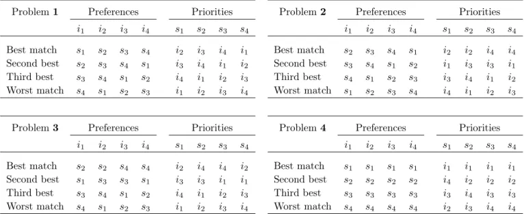
Problem 1 Preferences Priorities i1 i2 i3 i4 s1 s2 s3 s4 Best match s1 s2 s3 s4 i2 i3 i4 i1 Second best s2 s3 s4 s1 i3 i4 i1 i2 Third best s3 s4 s1 s2 i4 i1 i2 i3 Worst match s4 s1 s2 s3 i1 i2 i3 i4
Problem 2 Preferences Priorities i1 i2 i3 i4 s1 s2 s3 s4 Best match s2 s3 s4 s1 i2 i2 i4 i4 Second best s3 s4 s1 s2 i1 i3 i3 i1 Third best s4 s1 s2 s3 i3 i4 i1 i2 Worst match s1 s2 s3 s4 i4 i1 i2 i3
Problem 3 Preferences Priorities i1 i2 i3 i4 s1 s2 s3 s4 Best match s2 s2 s4 s4 i2 i4 i4 i2 Second best s1 s3 s3 s1 i3 i3 i1 i1 Third best s3 s4 s1 s2 i4 i1 i2 i3 Worst match s4 s1 s2 s3 i1 i2 i3 i4
Problem 4 Preferences Priorities i1 i2 i3 i4 s1 s2 s3 s4 Best match s1 s1 s1 s1 i1 i1 i1 i1 Second best s2 s2 s2 s2 i4 i2 i2 i2 Third best s3 s3 s3 s3 i3 i4 i3 i3 Worst match s4 s4 s4 s4 i2 i3 i4 i4
Table 1: Preferences of students over schools and priorities of schools over students.
We selected the four problems in such a way that a wide variety of situations is covered. In Problem 1, each student is ranked last in her most preferred, third in her second most preferred, second in her third most preferred, and first in her least preferred school. This problem thus resembles a situation where preferences (and priorities) are heterogeneous and the tension between the two sides of the market is maximal. The other extreme case, homogenous preferences (and priorities in the relevant parts) and no conflict between the two sides of the market, corresponds to Problem 4. Problems 2 and 3 are intermediate situations.
During the experiment, subjects assume the role of students. Schools are not strategic players. Given the information in Table 1, the subjects’ task in the static mechanisms is to submit a ranking over schools (not necessarily the true preferences) to be used by a central clearinghouse to assign students to schools. Subjects are free to submit a list of less than four schools. So, for example, a subject is allowed to submit the ranking s3, s1. We consider two static mechanisms,
the “student proposing deferred acceptance” (treatment CI) and the “school proposing deferred acceptance” (treatment CS) mechanisms. For the particular school choice settings at hand, the two mechanisms are as follows:
Static mechanisms (CI and CS) Step 1.
(CI) Each student sends an application to the school she ranked first. If a student did not list any school, then she will not send any application.
Each school temporarily accepts the applicant with the highest priority and rejects all other applicants.
(CS) Each school offers a seat to its highest priority student.
Each student temporarily accepts the school she likes best according to her submitted ranking and rejects all other offers.
Step 2.
(CI) Each student who got rejected in the previous step sends an application to her next highest ranked school. If there is no such school, then the student will not send any application.
Among the previously retained (if any) and new applications, each school temporarily accepts the applicant with the highest priority and rejects all other applicants.
(CS) Each school that got rejected in the previous step makes an offer to its next highest priority student.
Among the previously retained (if any) and new offers, each student temporarily accepts the school she likes best according to her submitted ranking and rejects all other offers.
Steps 3, 4, . . .
(CI) Step 2 is repeated until no more applications are rejected. Each student is assigned to the school that holds her application. If a student got rejected by all schools she ranked, she is left unmatched.
(CS) Step 2 is repeated until no more offers are rejected. Each student is assigned to the school she holds the offer from. If a student does not hold an offer, she is left unmatched. In our dynamic implementations students do not submit a ranking to the central clearinghouse. Instead, they go through each step of the corresponding static algorithm. So, while the static mechanisms induce a simultaneous move game, in the dynamic implementation subjects face a sequential move game. The descriptions of the dynamic versions of the student proposing DA mechanism (treatment DI) and the school proposing DA mechanism (treatment DS) are as follows:
Dynamic mechanisms (DI and DS) Phase 1.
(DI) Each student is asked to send an application that either contains the name of a school or is left empty. If a student decides to send an empty application, she will not be able to send future applications.
Each school temporarily accepts the applicant with the highest priority and rejects all other applicants.
Each student is informed about the status of the application, that is, if it is retained or whether it got rejected. If a student sent an empty application, she is informed that she did not obtain a seat.
(DS) Each school offers a seat to its highest priority student.
Each student decides to retain at most one of the offers received. Phase 2.
(DI) The students who sent an application to a school in the previous phase and got rejected are asked to send a new application (that consists of a school the student has not yet applied to or is left empty). If a student decides to send an empty application, she will not be able to send future applications.
Among the previously retained (if any) and new applications, each school temporarily accepts the applicant with the highest priority and rejects all other applicants.
Each student who sent a new application to a school and each student whose application was retained in the previous phase is informed about the status of the application, that is, if it is retained or whether it got rejected. Each student who sent an empty application is informed that she did not obtain a seat.
(DS) Whenever a school’s offer is rejected by a student, the school makes an offer to its next highest priority student.
Each student who received at least one new offer can retain at most one offer (among the new offers and the retained one, if it exists).
Phases 3, 4, . . .
(DI) Phase 2 is repeated until each student decides not to send any further application, has been rejected by all schools, or has her application retained by a school. Each student is assigned to the school that holds her application. If a student got rejected by all schools or sent an empty application, she is left unmatched.
(DS) Phase 2 is repeated until no more offers are rejected. Each student is assigned to the school she holds the offer from. If a student does not hold an offer, she is left unmatched. The experiment was programmed within the z–Tree toolbox provided by Fischbacher [15] and carried out at Lineex (www.lineex.es) hosted at the University of Valencia. In total, 192 under-graduates from various disciplines participated in the experiment. We run one session with 48 subjects per treatment. At the beginning of the session, subjects were anonymously matched into groups of four. Within each group, one subject was assigned the role of student i1, another subject
the role of i2, and so forth. Groups and roles did not change over the course of the experiment.
Participants were told that the experiment would take a total of 24 rounds and that preferences and priorities would change each six rounds. Before the first round, subjects went individually over an illustrative example in order to get used to the matching procedure. Afterwards, we implemented a trial period that was not taken into account for payment. This helped subjects to get familiar with the computer software. At the beginning of each round, the computer screen presented the preferences of all group members and the priorities of the four schools. Subjects took then their respective decisions. At the end of each round, subjects got to know the outcome of the matching process. In treatments DI and DS, due to the sequential nature of the game, subjects knew the status of their application at each point of the process. No explicit information about the behavior of the other group members was provided. At the end of the experiment, one round was randomly selected for payment. Subjects received 24, 20, 16, and 12 experimental currency units (ECU) if they ended up in their most, second most, third most, and least preferred school. They got 7 ECU if they remained unmatched. Each ECU was worth 1 Euro.2
3
Theory
In this section we start with the definition of a school choice problem and then provide a broad description of the extensive–form games induced by the two dynamic mechanisms, DI and DS. Since the two mechanisms differ in very important aspects, we then focus on each game in turn.
3.1
School choice problem
A school choice problem is a five-tuple hI, S, q, PS, PIi where
• I is a finite set of students (individuals). • S is a finite set of schools.
• qs= 1 for each s ∈ S, where qs is the number of seats at s ∈ S.
• PS = (Ps)s∈S is a profile of strict priority relations for schools, where Ps is a complete,
irreflexive, and transitive binary relation over I ∪ {s} for s ∈ S.
• PI = (Pi)i∈I is a profile of strict preference relations for students, where Pi is a complete,
irreflexive, and transitive binary relation over S ∪ {i} for i ∈ I.
We say that s ∈ S finds i ∈ I acceptable if and only if iPss and that i ∈ I finds s ∈ S acceptable
if and only if sPii. In the problems we consider, a matching of students to schools is a function
µ : I ∪ S → I ∪ S such that for all i ∈ I and s ∈ S: • µ(i) ∈ S ∪ {i},
• µ(s) ∈ I ∪ {s}, and
• s = µ(i) if and only if i = µ(s),
where the notation v = µ(v) means that agent v is unmatched under µ and v0 = µ(v) denotes that agent v0 is agent v’s partner under matching µ. We let M denote the set of matchings.
A matching µ is individually rational if and only if µ(v)Pvv for all v ∈ V . Moreover, we say
that a pair (i, s) blocks the matching µ if and only if sPiµ(i) and iPsµ(s). Since in the problems
we consider each school finds each student acceptable and likewise each student finds each school acceptable, every matching in M is individually rational. Therefore, we say that a matching is stable if there is no pair that blocks it. We denote by S(P ) the set of all stable matchings. The set of stable matchings is always non–empty (Gale and Shapley [16]). Moreover, for each problem, there is a student optimal stable matching that is weakly preferred by all students to any other stable matching in S(P ); similarly, there is a school optimal stable matching that is weakly preferred by all firms to any other stable matching in S(P ) (Gale and Shapley [16]).
3.2
General description of the extensive–form games
Given the definition of a school choice problem, we are now in a position to describe the extensive– form games agents play when confronted with the dynamic mechanisms, DI and DS. The extensive– form games are composed of the following elements:
• A set of actions Ai = S ∪ {i} for each student i. In DI, this set includes all possible proposals
that might potentially be made by i at some point in the game, including the “no school” option (modelled as proposing to oneself). In DS, choosing s means to hold the proposal from school s and to reject every other proposal that might have been received or held from a previous step, and to choose i means rejecting all proposals. We let A ≡ ∪i∈IAi.
• A set of nodes or histories X, where
– the initial node or empty history x0 is an element of X,
– each x ∈ X \ {x0} takes the form x = (a1, a2, ..., ak) for some finitely many actions
ai ∈ A, and
– if (a1, a2, ..., ak) ∈ X \ {x0} for some k > 1, then (a1, a2, ..., ak−1) ∈ X \ {x0}.
When x = (x0, a1, . . . , ak), k ≥ 1, we say that x0 is a predecessor of x.
We let A(x) ≡ {a ∈ A : (x, a) ∈ X} denote the set of actions available to a student whose turn it is to move after history x ∈ X. Clearly, we have A(x) ⊆ S ∪ {i} for all x ∈ X where it is student i’s turn to move.
• A set of end nodes E ≡ {x ∈ X : (x, a) /∈ X for all a ∈ A}.
• A function ι : X \ E → I that indicates whose turn it is to move at each decision node in X \ E.
We let Xi ≡ {x ∈ X \ E : ι(x) = i} denote the set of decision nodes belonging to student i.
• A partition = of the set of decision nodes X \ E, such that if x and x0 are in the same element
of the partition, then (i) ι(x) = ι(x0), and (ii) A(x) = A(x0). The information available to student ι(x) when, after history x, it is her turn to move is described by =(x), the element of the partition = that contains x.
We let =i ≡ {=(x) : x ∈ X \ E with ι(x) = i} denote the set of information sets belonging
to student i.
• An outcome function g : E → M that associates each terminal history with a matching. • For each student i ∈ I, a preference ordering Pi of schools.
We are now in a position to give a definition of a strategy in this extensive–form game.
Definition 1: A (pure) strategy for student i in this extensive–form game is a function σi : =i → A
such that σi(=(x)) ∈ A(x), for all x ∈ Xi.
Finally, even though we have provided a general description of the games induced by both DI and DS, they are clearly different mechanisms. For example, the set of actions available at a node x and the set of students allowed to move depend on the particular rules of the games induced by each mechanism. In Sections 3.3 and 3.4, we focus on each of these games in turn.
3.3
Game induced by DI
Two rules of DI, which we describe next, are of special importance.
Rule 1: In DI students cannot pass turns, i.e., if a student sends an application to “no school” at some step, she is not allowed to send applications at future steps.
Rule 2: In DI a student cannot send an application to a school more than once.
Whenever a student makes a new proposal it is because she was rejected and by Rule 2 she makes a new proposal to “no school” or to a school she has not proposed to before. Moreover, by Rule 1, after proposing to “no school” the student can no longer make proposals.
Therefore, in what the strategy of a student is concerned, her observed decisions induce an ordered list. Formally, consider student i, a profile of strategies σ = (σi, σ−i) leading to x ∈ E,
and let x1, . . . , xk, k ≥ 1, denote all the predecessors of x where student i proposes. Without loss
of generality, let xj be a predecessor of xj+1, j = 1, . . . , k − 1.
Definition 2: In the game induced by DI, the ordered list revealed by student i in the play of σ is Qσi = σi(=(x1)), . . . , σi(=(xk)), if σi(=(xk)) = i, and Qσi = σi(=(x1)), . . . , σi(=(xk)), i, otherwise.
Note that no two elements of this list are the same, so that this is a strict partial order of schools, having i as a last element. In fact, by Rule 1, i can only be the last element of this list and, by Rule 2, no school can appear twice.
Claim 1: The outcome of the game induced by DI when students use σ coincides with the outcome of the game induced by CI when students submit the ordered lists revealed in the play of σ. Proof. Immediate from the definition of ordered lists revealed in the play of a strategy profile and from the fact that DI emulates CI.
Still, the information revealed in the play of a strategy leading to a particular terminal node may only provide a partial order of schools, so that several (complete) orders may be compatible with it. Moreover, the strategy space is clearly much wider in DI than in CI, so that one strategy in DI may lead to different revealed ordered lists.
A class of strategies that deserves attention for its simplicity is the class of preference strategies. A student using a preference strategy always proposes to the best ranked school that she has not proposed to yet according to some preference ordering. Formally, consider student i, let Qi be
an ordered list of preferences over the elements of S ∪ {i}, and let maxQi(S
0) be the best ranked
element according to Qi in the set S0 ⊆ S ∪ {i}, with i ∈ S0.
Definition 3: In the game induced by DI, σi is a preference strategy if there exists an ordered list
Qi for student i such that for all x ∈ Xi, σi(=(x)) = maxQi(A(x)). In this case, we say that σi is
Remark 1: When student i uses the preference strategy consistent with Qi, the ordered list that
is revealed (at least partially) in any play of the game is Qi.
Claim 2: Every Nash equilibrium outcome in the game induced by CI is a Nash equilibrium outcome in the game induced by DI.
Proof. See the Appendix.
Haeringer and Klijn [18] show that every stable and possibly some unstable matchings (when the priority structure exhibits so-called Ergin cycles) can be sustained in Nash equilibrium in the game induced by CI. It therefore follows from Claim 2 that the same result holds in the game induced by DI.
Finally, whereas submitting the true preferences to the static mechanism is a weakly dominant strategy (Dubins and Freedman [10] and Roth [26]), the preference strategy consistent with the true preferences is not weakly dominant in the game induced by DI. In fact, when the other players use strategies that are not preference strategies, deviating from the preference strategy consistent with the true preferences may trigger the revelation of other, more favorable ordered lists by the other students and lead to a better outcome.
Claim 3: In the game induced by DI, the preference strategy consistent with the true preferences is in general not a weakly dominant strategy.
Proof. See the Appendix.
Additionally, in the game induced by DI, due to the lack of information on others’ moves (as the game proceeds a student remembers her own proposals and schools’ reactions to these proposals), there are very few proper subgames, and those that do exist appear only at the end of the tree. It follows that the concept of subgame perfect Nash equilibrium does not allow us to refine the set of predicted outcomes either and our best prediction for the obtained matchings is a superset of the Nash equilibrium outcomes in the game induced by CI.
3.4
Game induced by DS
It is a well known fact that the set of Nash equilibrium outcomes of the game induced by CS when each school has one seat coincides with the set of stable matchings (Gale and Sotomayor [16], Roth [27]). In the following Claim, we show that the set of Nash equilibrium outcomes in the game induced by DS coincides with the set of stable matchings and, therefore, with the set of Nash equilibrium outcomes in the game induced by CS.
Claim 4: The set of Nash equilibrium outcomes in the game induced by DS coincides with the set of stable matchings.
The following rule of DS is of special importance.
Rule 3: In DS once a student holds the proposal of a school, she can only reject it upon receiving and holding another school’s proposal.
Since in the game induced by DS a student can receive a proposal from a school at most once, we can guarantee that the decisions made by a student along the path of a play reveal a strict partial order of schools. Moreover, each school whose proposal is held by a student is revealed to be better than being unmatched in which case, by Rule 3, being unmatched cannot be revealed preferred to being assigned to that school. Therefore, the rules of the game guarantee that transitivity can never be violated. Formally, consider student i, a profile of strategies σ = (σi, σ−i) leading to
x ∈ E, and let S0 be the set of schools held by student i in the course of play of σ. Definition 4: The ordered list that is revealed by student i in the play of σ is Qσ
i = i, when S 0 = ∅,
and is Qσ
i = s0k, . . . , s 0
1, i, where s0j ∈ S0, j = 1, . . . , k, is the jth school whose proposal is held by i
in the course of play of σ.
Claim 5: The outcome of the game induced by DS when students use σ coincides with the outcome of the game induced by CS when students submit the ordered lists revealed in the play of σ. Proof. Immediate from the definition of ordered lists revealed in the play of a strategy profile and from the fact that DS emulates CS.
As it happens in the game induced by DI, the class of preference strategies is of particular interest. A student using a preference strategy always holds the proposal from the best ranked school in some ordered list of schools among those schools that propose at some step and the school whose proposal may be held from a previous step (if any). Formally, consider student i and let Qi
be an ordered list over the elements of S ∪ {i}.
Definition 5: In the game induced by DS, σi is a preference strategy for student i if there exists
an ordered list Qi such that for all x ∈ Xi, σi(=(x)) = maxQi(A(x)). In this case, we say that σi
is the preference strategy consistent with Qi
Preference strategies are a natural form of behavior and Claim 6 refers to a particular subclass, the subclass of preference strategies consistent with a truncation of the true preferences.
In the game induced by CS, a student employs a truncation strategy if she removes a tail of least preferred partners from the true preference list. For example, if the true ranking is s2, s3, s4, s1,
then s2, s3 is a truncation strategy, but s2, s4 is not. In the game induced by CS, truncations may
play an important role given that, for each strategy a student may use, the induced match can be replicated or improved upon by some truncation of the true preferences of the student (Roth and Vande Vate [28]). This fact, together with Claim 5 imply that, in the game induced by DS, given a profile of preference strategies for the students other than i, there is a best reply for i that consists of a preference strategy consistent with a truncation of the true preferences.
Nevertheless, for some profiles of strategies of the other players (including strategies other than preference strategies), there is no strategy consistent with a truncation of the true preferences that can be a best reply in DS. Therefore, contrary to what happens in CS, when choosing a best reply, agents cannot restrict to the class of truncations.
Claim 6: Consider the game induced by DS. Given a strategy–profile of all but one student i, there need not be a best reply of student i that is a preference strategy consistent with a truncation of her true preferences.
Proof. See the Appendix.
Finally, we can also show that, as it happens in DI, given the low level of information on other players’ chosen strategies, the game induced by DS has very few subgames and subgame perfect Nash equilibrium does not give us sharper predictions on the possible outcomes. Therefore, in the game induced by DS, the set of subgame perfect Nash equilibrium outcomes coincides with the set of Nash equilibrium outcomes.
4
Experimental results
We now present the results of our experiment. First, we analyze the behavior of the subjects (Section 4.1). Afterwards, we show how behavior affects stability (Section 4.2) and welfare (Section 4.3).
4.1
Behavior
Dubins and Freedman [10] and Roth [26] show that subjects have incentives to reveal preferences truthfully in treatment CI. Nevertheless, it is well documented in the experimental literature that agents do not always realize that it is in their best interest to reveal their true preferences when confronted with centralized strategy–proof mechanisms (see, e.g., Calsamiglia et al. [4], Chen and Kesten [6], Chen and Sönmez [9], Featherstone and Niederle [14], Guillen and Hing [17], Klijn et al. [22],[23], and Pais and Pintér [25]). We analyze whether a dynamic implementation of the student proposing DA algorithm where, as the algorithm proceeds, subjects receive feedback about their previous applications and corresponding decisions, mitigates or aggravates this problem.
Given some student’s true preferences, we write skfor the school that is ranked in k-th position (from best to worst), i.e., the k-th best school. For example, if the student’s true ranking is s2, s3, s4, s1, then s4 = s1.
Consider the mechanism CI. Haeringer and Klijn [18] show that a strategy that does not rank all schools is weakly dominated. Now suppose a student ranks all schools. Haeringer and Klijn [18] show that a strategy that for some i < j ranks school sj somewhere above/before school si is weakly dominated by a strategy that is obtained by switching sj and si back in the (true) relative order. Therefore, the number of such switches can be employed to measure a subject’s degree of
(ir)rationality. For example, if the true ranking is s2, s3, s4, s1 and a subject reports in treatment
CI the list s4, s2, she switches schools s1 and s3 and schools s2 and s3. But we do not have any
information on how she for instance relates schools s2 and s4.
Now consider the mechanism DI. Obviously the induced game has a much richer structure than that of CI. In particular, strategies can be much more complex. And, in fact, by Claim 3, the preference strategy consistent with the true preferences need not be weakly dominant. For this reason, we expect at least as many switches —i.e., situations in which a student first proposes to a school sj and in a later step to a better school si (i < j)— as in the case of CI, except that now we
should take into account that there is only limited information about the student’s strategy. More precisely, we will often not be able to determine whether a subject would make an irrational switch, simply because the game has not reached a situation in which this could happen/be observed. HYPOTHESIS 1A: Subjects switch pairs weakly more often in treatment DI than in treatment CI.
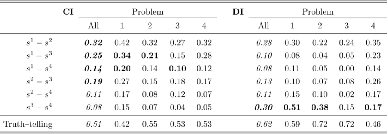
Table 2 presents for each i, j with i < j in row si− sj the frequency with which (the better)
school si is switched with (the worse) school sj.
CI Problem DI Problem All 1 2 3 4 All 1 2 3 4 s1− s2 0.32 0.42 0.32 0.27 0.32 0.28 0.30 0.22 0.24 0.35 s1− s3 0.25 0.34 0.21 0.15 0.28 0.10 0.08 0.04 0.05 0.23 s1− s4 0.14 0.20 0.14 0.10 0.12 0.08 0.11 0.05 0.00 0.14 s2− s3 0.19 0.27 0.15 0.18 0.17 0.13 0.10 0.07 0.08 0.26 s2− s4 0.11 0.17 0.08 0.12 0.07 0.11 0.15 0.10 0.02 0.17 s3− s4 0.08 0.15 0.07 0.04 0.05 0.30 0.51 0.38 0.15 0.17 Truth–telling 0.51 0.42 0.55 0.53 0.53 0.62 0.59 0.72 0.72 0.46
Table 2: Frequencies that two schools are switched under the static (left) and dynamic (right) student proposing DA mechanisms. Significant treatment effects obtained from panel data regressions with in-dividual random effects are indicated in boldface for the treatment with the higher frequency. We also display the frequency of subjects that cannot be rejected to tell the truth.
The left part of the table shows that subjects often switch pairs in treatment CI. Also, in each of the four problems, the switching frequency is highest for the pair s1− s2 and lowest for the pair
s3 − s4. A comparison with the right part of the table reveals that switching frequencies tend to
be lower in treatment DI. For example, in Problems 1-3 there are very few subjects who apply to their third best or worst school without having applied before to their most preferred or second most preferred school. Consequently, it is no surprise that the switching frequencies for several of the pairs involving s1 are significantly higher in treatment CI. On the other hand, we can also see that in Problems 1,2, and 4, subjects switch the pair s3− s4 significantly more often in treatment
DI than in treatment CI. Finally, and with respect to the aggregated data, we find that the pairs s1 − s2, s1 − s3, s1 − s4, and s2− s3 are switched more often in treatment CI than in treatment
DI, while the pair s3− s4 is switched more often in treatment DI than in treatment CI.
Table 2 also shows the frequencies with which subjects cannot be rejected to tell the truth. In treatment CI this is equal to determining the frequencies that subjects submit lists equal to their true preferences, while we calculate in treatment DI the frequencies whether subjects “go down the list” (a subject applies first to her most preferred school; then, if she got rejected at some point of the game, an application to the second most preferred school is submitted; and so forth, until the game stops). One observes higher frequencies in treatment DI for Problems 1-3, which is due to two effects: subjects switch less pairs in these problems in treatment DI and frequencies are ex ante biased towards treatment DI since not all of the possible comparisons are observed in this treatment.
Result 1A: With the exception of the pairs s2− s4 and s3− s4, subjects switch pairs more often in
treatment CI than in treatment DI. Moreover, in Problems 1-3 there are substantially more subjects who cannot be rejected to tell the truth in treatment DI than in treatment CI.
The static school proposing mechanism differs from the static student proposing mechanism in that students have now incentives to manipulate. In the dynamic implementation of the school proposing mechanism we would like to find out whether subjects understand that truth–telling might not always be optimal. More specifically, as a natural counterpart to Hypothesis 1A, we now seek to study whether and how a dynamic implementation of the school proposing DA algorithm may change subjects’ behavior.
Consider the mechanism CS. As mentioned in Section 3.4, a notable class of manipulations is that of strategies that involve a truncation of the true preferences. Obviously, truncation strategies have a very simple structure relative to the true preferences. But maybe more importantly, the set of truncation strategies is known to be strategically exhaustive, i.e., each school a student is matched to when manipulating her preferences can be obtained or strictly improved upon by using some truncation strategy (Roth and Vande Vate [28]). Truncation strategies have been observed in practice, for instance, in the sorority rush (Mongell and Roth [24]). Therefore, it is of interest to determine to which extent subjects employ truncation strategies in our experiment.
Now consider the mechanism DS. Similarly to the previous discussion on CI and DI, the mech-anism DS induces a much richer game than CS. Additionally, according to Claim 6, the class of preference strategies consistent with truncations need not be strategically exhaustive. Therefore, we expect subjects to truncate weakly less often in treatment DS than in treatment CS. We do note however that there is only limited information about the students’ strategies in treatment DS. More precisely, we are often not able to determine whether a subject employs a strategy based on a truncated list, simply because the game has not reached a situation in which this could be concluded.
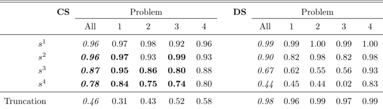
First, it turns out that under CS subjects switch pairs with frequencies that are similar to those presented in Table 2 for treatment CI, while under DS almost no subject accepts an offer from a school sj after having temporarily accepted before an offer from a more preferred school si (i < j).
In fact, aggregated over all problems and pairs si− sj (i < j), the switching frequency is 25% in
treatment CS but only 2% in treatment DS.
We now present in Table 3 the frequencies that an offer from a school is acceptable. More precisely, for CS we consider the frequency that a school is ranked in the submitted list. For DS we consider the frequency that an offer from a school is accepted in some step of the algorithm conditional on that the subject does not hold an offer from another school.
CS Problem DS Problem All 1 2 3 4 All 1 2 3 4 s1 0.96 0.97 0.98 0.92 0.96 0.99 0.99 1.00 0.99 1.00 s2 0.96 0.97 0.93 0.99 0.93 0.90 0.82 0.98 0.82 0.98 s3 0.87 0.95 0.86 0.80 0.88 0.67 0.62 0.55 0.56 0.93 s4 0.78 0.84 0.75 0.74 0.80 0.44 0.45 0.44 0.02 0.83 Truncation 0.46 0.31 0.43 0.52 0.58 0.98 0.96 0.99 0.97 0.99
Table 3: Frequencies that a school is acceptable under the static (left) and dynamic (right) school propos-ing DA mechanisms. Significant treatment effects obtained from panel data regressions with individual random effects are indicated in boldface for the treatment with the higher frequency. We also display the frequency of subjects that cannot be rejected to use a truncation strategy.
The table shows that only a few schools are declared unacceptable in the static school proposing DA mechanism. Also, the data for this mechanism is consistent in the sense that for all i < j, the frequency that school si is accepted is greater than or equal to the frequency with which school sj is accepted (the only exception is the pair s1−s2 in Problem 3). This consistency can also be found
in treatment DS, but, most importantly, the acceptance rates of s2, s3, and s4 are substantially
lower in Problems 1-3. Hence, it is no surprise that the aggregated acceptance rates for those schools are significantly lower in treatment DS than in treatment CS.
In the last row of Table 3 we display the frequency of subjects that cannot be rejected to use a truncation strategy (which nonetheless take different meanings in the treatments CS and DS). We see that only a few subjects can be rejected to play truncation strategies in treatment DS. Recall that the information we can collect from the decisions of the subjects in treatment DS is limited due to the nature of the mechanism. For example, if a subject initially receives only an offer from s2 that she accepts and rejects later on offers from s3 and s4, we can only conclude that
the ordered list of preferences revealed by this subject in the play of the game includes s2 and that s2 is better ranked than both s3 and s4, but we do not know how s3 and s4 compare and whether these two schools would be accepted in case the subject was not holding s2’s proposal in the first
place. Since there are many truncation strategies that are consistent with the supposed behavior, we cannot reject that she behaves according to a truncation. This is different for a subject who rejects an offer from s2 in the first step of the algorithm and temporarily accepts an offer from s3
in the second step. Such a subject’s strategy is clearly not a preference strategy consistent with a truncation of the true preferences.
Result 1B: In Problems 1-3 subjects accept offers from low ranked schools significantly less often in treatment DS than in treatment CS. Moreover, there are substantially more subjects who cannot be rejected to play truncation strategies in treatment DS than in treatment CS.
4.2
Stability
Stability is the central solution concept in matching markets. In the problems we consider, a matching is said to be “blocked” if there is a student that prefers to be assigned to some school with a slot that is either available or occupied by another student with a lower priority. Then, a matching is “stable” if no student can form a blocking pair with any school. Problem 1 has four stable matchings. In the student optimal stable matching, which is obtained in treatments CI and DI when all students reveal their preferences truthfully, each student is assigned to her top school. Similarly, the school optimal stable matching, the matching obtained in treatments CS and DS under truth–telling, is such that each student is assigned to her worst school. In the two “compromise” stable matchings all students are assigned to their second most and third most preferred school, respectively. Problem 2 has 3 and Problem 3 has 2 stable matchings. Finally, there is one stable matching in Problem 4 (where for each k = 1, . . . , 4, student ik is matched to
school sk) and all four mechanisms coincide under truth–telling.
There is no reason to expect that stability is higher under the dynamic implementations of the mechanisms. In fact, according to Claim 2, all Nash equilibrium outcomes in CI (which includes all stable and possibly some unstable matchings) can also be sustained in Nash equilibrium in the game induced by DI. Moreover, according to Claim 4, the set of Nash equilibrium outcomes of the game induced by DS is the set of stable matchings which hence coincides with the set of Nash equilibrium outcomes in CS.
HYPOTHESIS 2: The frequency of stable matchings is not higher under the dynamic implemen-tations.
Nevertheless, we have already seen that, for Problems 1-3, the likelihood of switching pairs of schools in the student proposing mechanisms and of behaving in a way consistent with a truncation of the true preferences in the school proposing mechanisms depends on whether we consider the static or the dynamic implementations. We now analyze whether and how these different behaviors affect the rates of stable outcomes.
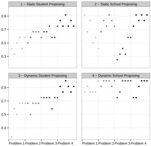
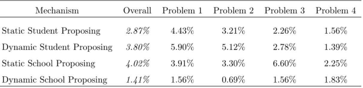
Figure 1 plots the frequency with which a stable matching is reached over the course of the experiment.
● ● ● ● ● ● ● ● ● ● ● ● ● ● ● ● ● ● ● ● ● ● ● ● ● ● ● ● ● ● ● ● ● ● ● ● ● ● ● ● ● ● ● ● ● ● ● ● ● ● ● ● ● ●● ● ● ● ● ●● ● ● ● ● ● ● ● ● ● ● ● ● ● ● ● ● ● ● ● ● ● ● ● ● ● ● ● ● ● ● ● ● ● ● ●
1 − Static Student Proposing 2 − Static School Proposing
3 − Dynamic Student Proposing 4 − Dynamic School Proposing 0.3 0.5 0.7 0.9 0.3 0.5 0.7 0.9
Problem 1 Problem 2 Problem 3 Problem 4 Problem 1 Problem 2 Problem 3 Problem 4
Figure 1: Frequencies of stable matchings. Since the number of stable matchings ranges from 1 (Problem 4) to 4 (Problem 1), comparisons across problems are meaningless.
There are stark differences between the treatments. The dynamic school proposing DA mech-anism seems to perform best among all four mechmech-anisms. In Problems 1-3 it visibly outclasses not only its natural peer, the static school proposing DA mechanism, but also the two student proposing DA mechanisms. On the other hand, there are hardly any differences between the two student proposing DA mechanisms. This intuition is confirmed if we look at the overall frequencies of stable matchings (63.89% in treatment CI, 68.08% in treatment DI, 70.49% in treatment CS, and 90.01% in treatment DS).
We run four random effects estimations, one for each problem, to assess treatment differences (Table 4). Our explanatory variables are three dummy variables that identify the different treat-ments: the variable “Student proposing” (β2) takes value 1 in treatments CI and DI and 0 in
treatments CS and DS, the variable “Static” (β3) takes value 1 in treatments CI and CS and 0
in treatments DI and DS, and the variable “Student proposing × Static” (β4) takes value 1 in
treatment CI and 0 in the other three treatments. Since each problem is played six times, we also include the variable “Repetition” (which takes values from 1 to 6) in order to account for
learn-ing effects within a problem. In this settlearn-ing, differences across treatments are evaluated against treatment DS which serves as a benchmark. In particular, β3 measures the differences between
treatments CS and DS, while β3 + β4 assesses the difference between treatments CI and DI.
Problem 1 Problem 2 Problem 3 Problem 4 Constant (β0) 0.8354∗∗∗ 0.9139∗∗∗ 0.8326∗∗∗ 0.8444∗∗∗ (0.0862) (0.0487) (0.0640) (0.0069) Repetition (β1) 0.0113 0.0167 0.0280∗ 0.0017 (0.0203) (0.0126) (0.0127) (0.0013) Student proposing (β2) −0.3333∗∗∗ −0.3194∗∗ −0.2083 −0.0001 (0.0927) (0.1183) (0.1107) (0.0058) Static (β3) −0.2222∗∗ −0.1806∗∗ −0.5139∗∗∗ −0.0042 (0.0697) (0.0620) (0.1039) (0.0068) Student proposing × Static (β4) 0.1528 0.1389 0.4583∗ −0.0055
(0.1340) (0.1605) (0.1856) (0.0112)
R2 0.0648 0.0458 0.0701 0.0155
Observations 1152 1152 1152 1152
Table 4: Random effects estimations on the frequency of reaching a stable matching. Errors are clustered on matching groups. ∗∗∗indicates significance at p = 0.001 (two-sided),∗∗indicates significance at p = 0.01 (two-sided), and∗ indicates significance at p = 0.05 (two-sided). The qualitative insights remain the same if we employ probit estimations.
In consistence with Figure 1, the value of β3 in Table 4 is significantly smaller than 0 in
Problems 1-3; that is, the likelihood of reaching a stable matching in treatment DS is higher than in treatment CS (by 22 percentage points in Problem 1, 18 percentage points in Problem 2, and 52 percentage points in Problem 3). Next, we apply χ2-tests to see whether the value of β3+ β4 is
significantly different from zero. Since this hypothesis is rejected at p = 0.05 in all four problems, there are no treatment differences between CI and DI.
Mechanism Overall Problem 1 Problem 2 Problem 3 Problem 4
Static Student Proposing 2.87% 4.43% 3.21% 2.26% 1.56% Dynamic Student Proposing 3.80% 5.90% 5.12% 2.78% 1.39% Static School Proposing 4.02% 3.91% 3.30% 6.60% 2.25% Dynamic School Proposing 1.41% 1.56% 0.69% 1.56% 1.83%
Table 5: Frequencies of blocking pairs.
pairs that can block a resulting matching. The data shows that fewer blocking pairs can be formed under the static student proposing DA mechanism than under the dynamic student proposing DA mechanism (the only exception is Problem 4) and that the dynamic implementation outper-forms the static implementation when the school proposing DA mechanism is employed (the only exception is again Problem 4). The overall difference between the static and the dynamic imple-mentation is considerably larger for the school than for the student proposing DA mechanism (2.61 percentage points versus 0.93 percentage points), which reaffirms our findings from the regressions that differences are only significant for the school proposing mechanism.
Result 2: The frequency of stable matchings is the same for treatments CI and DI. In Problems 1-3, the frequency of stable matchings is significantly higher in treatment DS than in treatment CS.
4.3
Welfare
For the dynamic mechanisms to be reasonable alternatives for the standard static mechanisms, it is crucial that decisions under the former mechanisms also translate into higher payoffs. And, given the results above that compare the set of Nash equilibrium outcomes in the dynamic and static mechanisms, there is a priori no reason to expect that the dynamic implementations present an improvement over their static counterparts in this dimension. In fact, switching the order of schools is a weakly dominated strategy in CI and the unique Nash equilibrium outcome in undominated strategies in this mechanism is the student optimal stable matching, which maximizes total payoffs in all problems. By contrast, there are no weakly dominant strategies in DI and the set of equilibrium outcomes is a superset of the set of stable matchings (Claim 2), thus containing inefficient matchings. On the other hand, in what the school proposing mechanisms are concerned, by Claim 4, the set of Nash equilibrium outcomes in both mechanisms equals the set of stable matchings. Moreover, if all subjects use truncation strategies in CS —which are know to be strategically exhaustive under this mechanism— a stable matching is obtained as long as subjects do not truncate above their partners under the student optimal stable. In fact, by truncating, stable matchings that correspond to higher average payoffs may be obtained.
HYPOTHESIS 3: Average payoffs are not higher under the dynamic implementations.
Nevertheless, with respect to the school proposing DA mechanisms, there are only very few subjects who can be rejected to play a preference strategy consistent with a truncation of the true preferences in treatment DS compared to treatment CS (Result 1B). And, with respect to the student proposing DA mechanisms, we have seen in Result 1A that all pairs except for s2− s4 and s3− s4 are switched
less often in treatment DI than in treatment CI. The fact that subjects actually switch less (or act according to the true preferences more often) under DI, may imply that the student optimal stable matching is obtained more often than what theoretic results imply, so that welfare levels may be higher than expected.
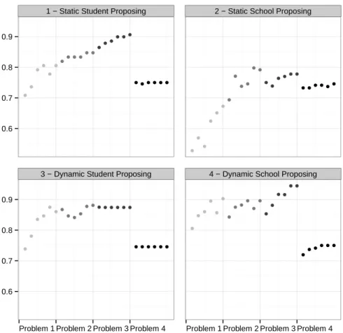
● ● ●● ● ●● ● ● ●● ● ●● ● ● ● ● ● ● ● ● ● ● ● ● ● ● ● ● ● ● ●● ● ● ● ● ● ●● ● ● ●● ● ● ● ● ● ●● ● ●● ● ●● ● ●● ● ● ● ● ● ● ● ● ● ● ● ● ●● ● ● ● ● ● ● ● ● ● ● ● ● ● ● ● ● ● ●● ● ●
1 − Static Student Proposing 2 − Static School Proposing
3 − Dynamic Student Proposing 4 − Dynamic School Proposing 0.6 0.7 0.8 0.9 0.6 0.7 0.8 0.9
Problem 1 Problem 2 Problem 3 Problem 4 Problem 1 Problem 2 Problem 3 Problem 4
Figure 2: Relative payoffs per round in each of the four treatments. The student (school) optimal stable matching leads to a relative payoff of 1 (0.5) in Problem 1, 1 (0.67) in Problem 2, 0.92 (0.67) in Problem 3, and 0.75 (0.75) in Problem 4.
Figure 2 plots the relative payoffs over the course of the experiment. In this figure, a value of 0.7 indicates that a subject earned on average 70% of her maximal payoff of 24 ECU. Since it is not always possible to assign all students to their most preferred school, comparisons across problems should be taken with care.
We can make three main observations. First, there are hardly any differences between the four mechanisms in Problem 4. Second, the dynamic school proposing DA mechanism leads to substantially higher payoffs than the static school proposing DA mechanism in Problems 1-3. And third, the two student proposing DA mechanisms perform similarly in Problems 1-3. Finally, aggregated over all problems, relative payoffs are 0.8112 in treatment CI, 0.8259 in treatment DI, 0.7139 in treatment CS, and 0.8472 in treatment DS. This is suggestive evidence that over the course of the experiment the dynamic implementation of the school proposing DA mechanism performs not only better than the static school proposing DA mechanism, but also does not yield lower payoffs than the two student proposing mechanisms.
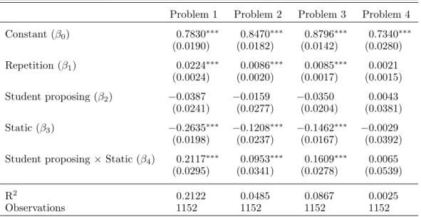
To see whether these visual insights are confirmed, we run again random effects regressions, using the same explanatory variables as in the subsection on stability (Table 6).
Problem 1 Problem 2 Problem 3 Problem 4 Constant (β0) 0.7830∗∗∗ 0.8470∗∗∗ 0.8796∗∗∗ 0.7340∗∗∗ (0.0190) (0.0182) (0.0142) (0.0280) Repetition (β1) 0.0224∗∗∗ 0.0086∗∗∗ 0.0085∗∗∗ 0.0021 (0.0024) (0.0020) (0.0017) (0.0015) Student proposing (β2) −0.0387 −0.0159 −0.0350 0.0043 (0.0241) (0.0277) (0.0204) (0.0381) Static (β3) −0.2635∗∗∗ −0.1208∗∗∗ −0.1462∗∗∗ −0.0029 (0.0198) (0.0237) (0.0167) (0.0392) Student proposing × Static (β4) 0.2117∗∗∗ 0.0953∗∗∗ 0.1609∗∗∗ 0.0065
(0.0295) (0.0341) (0.0278) (0.0539)
R2 0.2122 0.0485 0.0867 0.0025
Observations 1152 1152 1152 1152
Table 6: Random effects estimations on the relative payoff per subject. Errors are clustered on matching groups. ∗∗∗ indicates significance at p = 0.001 (two-sided),∗∗indicates significance at p = 0.01 (two-sided), and ∗ indicates significance at p = 0.05 (two-sided).
Supporting the conclusions drawn from the observation of Figure 2, the expected payoff of a subject in Problem 4 is the same in all four treatments and very close to the expected payoff associated with the unique stable matching, namely 0.75 (=18 ECU). More importantly, we can see that in Problems 1-3, the value of β3 is negative and significantly different from zero at p = 0.001;
that is, payoffs in these problems are higher in treatment DS than in treatment CS (by 6.32 ECU in Problem 1, 2.90 ECU in Problem 2, and 3.51 ECU in Problem 3). The payoff difference between CS and DS in Problem 1 is particularly high. Finally, we apply χ2-tests to see whether there are
differences between treatments CI and DI. We find for Problem 1 that payoffs are significantly higher in treatment DI at p = 0.05. The corresponding payoff difference is 1.24 ECU. There are no significant payoff differences between CI and DI for Problems 2 and 3.
Result 3: In Problems 1-3, payoffs are significantly higher in treatment DS than in treatment CS. In Problem 1, payoffs are significantly higher in treatment DI than in treatment CI.
5
Conclusion
Abdulkadiroğlu and Sönmez [1] show that the student proposing DA mechanism has nice theoretical properties in that revealing one’s preferences truthfully is a weakly dominant strategy in the
induced static game, so that the student optimal stable matching is obtained as a consequence. However, when the mechanism is brought to the laboratory it is commonly found that untrained subjects behave strategically even though they should not. It is thus the objective of this paper to analyze whether better experimental outcomes can be obtained if, instead of submitting lists, subjects make decisions dynamically by going through each of the underlying matching algorithms. Our theoretical results for the dynamic student proposing DA mechanism show that if players use a “going down the list” strategy, that is, they take a ranking of schools (that may or may not coincide with their true preferences) and always send an application to the better ranked school they have not yet applied to, then the outcome is equal to the outcome of the static game when the corresponding lists are submitted to the central planner. But since the dynamic game allows for richer strategies, it is not true that going down the list with respect to one’s true preferences is a weakly dominant strategy, so that in a laboratory experiment a wider range of behavior could be expected under the dynamic implementation. We nevertheless find experimentally that subjects tend to switch fewer pairs of schools at the top of their true preference under the dynamic implementation of the student proposing DA mechanism, even though these differences are not strong enough to substantially affect outcomes in terms of stability (63.89% in the static and 68.08% in the dynamic mechanism) and relative efficiency (0.8112 in the static and 0.8259 in the dynamic mechanism).
We also consider the static and the dynamic school proposing DA mechanisms. Students typically have incentives to manipulate the static mechanism, for instance by using truncation strategies, which are strategically exhaustive in this context. Since there are truncation strategies that are a best reply under the static but not under the dynamic mechanism, theoretically a wider range of behavior can again be supported for the dynamic implementation. Perhaps surprisingly, we find in our laboratory experiment that the dynamic school proposing DA mechanism does not only outperform the corresponding static implementation in terms of stability (70.49% in the static and 90.01% in the dynamic mechanism) and relative efficiency (0.7139 in the static and 0.8472 in the dynamic mechanism), but also the two student proposing DA mechanisms. This is because if an offer from some school is temporarily accepted under the dynamic implementation, subjects do not switch that school for a worse one later on, which is crucial for preventing unstable outcomes to occur. The overall switching frequency in the static implementation, on the other hand, is with 25% rather high and close to that of the static student proposing DA mechanism. Moreover, it is only under the dynamic school proposing DA mechanism that subjects learn that it can be worthwhile in terms of payoffs to reject offers from less desirable schools.
References
[1] A Abdulkadiroğlu and T Sönmez (2003). School choice: A mechanism design approach. Amer-ican Economic Review 93(3): 729–747.
[2] O Aygün and I Bó (2014) College admission with multidimensional privileges: The Brazilian affirmative action case. Working Paper, WZB Berlin Social Science Center.
[3] I Bó and R Hakimov (2016). Iterative versus standard deferred acceptance: Experimental evidence. Working Paper, WZB Berlin Social Science Center.
[4] C Calsamiglia, G Haeringer, and F Klijn (2010). Constrained school choice: An experimental study. American Economic Review 100(4): 1860–1874.
[5] M Castillo and A Dianat (2016). Information effects in the dynamic Gale–Shapley mechanism: An experimental study. Working Paper, Interdisciplinary Center for Economic Science, George Mason University.
[6] Y Chen and O Kesten (2016). Chinese college admissions and school choice reforms: An experimental study. Working Paper, University of Michigan.
[7] Y Chen and O Kesten (2016). Chinese college admissions and school choice reforms: A theo-retical analysis. Journal of Political Economy, forthcoming.
[8] L Chen and J Pereyra (2015). Time–constrained school choice. ECARES Working Paper. [9] Y Chen and T Sönmez (2006). School choice: An experimental study. Journal of Economic
Theory 127(1): 202–231.
[10] L Dubins and D Freedman (1981). Machiavelli and the Gale-Shapley algorithm. American Mathematical Monthly 88(7): 485–494.
[11] U Dur, R Hammond, and T Morrill (2016). Identifying the harm of manipulable school-choice mechanisms. Working Paper, North Carolina State University.
[12] F Echenique, A Wilson, and L Yariv (2016). Clearinghouses for two-sided matching: An experimental study. Quantitative Economics 7(2): 449–482.
[13] C Featherstone and E Mayefsky (2015). Why do some clearinghouses yield stable outcomes? Experimental evidence on out-of-equilibrium truth–telling. Working Paper, The Wharton School, University of Pennsylvania.
[14] C Featherstone and M Niederle (2013). Improving on strategy-proof school choice mechanisms: An experimental investigation. Working Paper, Stanford University.
[15] U Fischbacher (2007). z-Tree: Zurich toolbox for ready-made economic experiments. Experi-mental Economics 10(2): 171–178.
[16] D Gale and M Sotomayor (1985). Ms Machiavelli and the stable matching problem. American Mathematical Monthly 92(4): 261–268.
[17] P Guillen and A Hing (2014). Lying through their teeth: Third party advice and truth telling in a strategy proof mechanism. European Economic Review 70(1): 178–185.
[18] G Haeringer and F Klijn (2009). Constrained school choice. Journal of Economic Theory 144(5): 1921–1947.
[19] I Hafalir, R Hakimov, D Kübler, and M Kurino (2014). College admissions with entrance exams: Centralized versus decentralized. Working Paper, Tepper School of Business, Carnegie Mellon University.
[20] E Haruvy and U Ünver (2007). Equilibrium selection and the role of information in repeated matching markets. Economics Letters 94(2): 284–289.
[21] P Jaramillo, Ç Kayı, and F Klijn (2014). On the exhaustiveness of truncation and dropping strategies in many-to-many matching markets. Social Choice and Welfare 42(4): 793–811. [22] F Klijn, J Pais, and M Vorsatz (2013). Preference intensities and risk aversion in school choice:
A laboratory experiment. Experimental Economics 16(1): 1–22.
[23] F Klijn, J Pais, and M Vorsatz (2016). Affirmative action through minority reserves: An experimental study on school choice. Economics Letters 139: 72–75.
[24] S Mongell and A Roth (1991). Sorority rush as a two-sided matching mechanism. American Economic Review 81(3): 441–464.
[25] J Pais and Á Pintér (2008). School choice and information: An experimental study on match-ing mechanisms. Games and Economic Behavior 64(1): 303–328.
[26] A Roth (1982). The economics of matching: Stability and incentives. Mathematics of Opera-tions Research 7(4): 617–628.
[27] A Roth (1984). Misrepresentation and stability in the marriage problem. Journal of Economic Theory 34(2): 383–387.
[28] A Roth and J Vande Vate (1991). Incentives in two-sided matching with random stable mech-anisms. Economic Theory 1(1): 31–44.