DOI: 10.1590/1808-057x201805810
Original Article
Bank revenue diversification: its impact on risk and return in
Brazilian banks
Jorge H. L. Ferreira1
https://orcid.org/0000-0002-9128-8411 Email: jhlopes@unisinos.br
Francisco A. M. Zanini2 Email: fzanini@unisinos.br
Tiago W. Alves2 Email: twa@unisinos.br
1 Banco do Estado do Rio Grande do Sul, Unidade de Reestruturação de Crédito, Porto Alegre, RS, Brazil
2 Universidade do Vale do Rio dos Sinos, Escola de Gestão e Negócios, Departamento de Ciências Contábeis, São Leopoldo, RS, Brazil
Received on 07.02.2017 – Desk acceptance on 07.26.2017 – 3rd version approved on 01.18.2018 – Ahead of print on 09.11.2018
Associate Editor: Fernanda Finotti Cordeiro Perobelli
ABSTRACT
The present study aims to determine the impact of bank revenue diversification on Brazilian banks’ risk and return. This strategy has been adopted by banks in several countries, including Brazil. In 2003, noninterest income accounted for 17.80% of the operating revenue of the banks analyzed, and in 2014, this share increased to 27.40%. While many studies have addressed the subject in American, European and Asian banks, it still has not been approached in a sample of Brazilian banks. Since the banking industry is a key variable for the financial system’s stability, it is important to study the factors that affect banks’ risk and return. We analyzed the sample for the period from 2003 to 2014, using dynamic panel data GMM (Generalized Method of Moments) to address endogeneity, heteroscedasticity and autocorrelation problems. Our main results show that noninterest income has a major role in the performance of the banks studied; our analysis of financial intermediation activities showed that loan operations produced better results than trading. Moreover, confirming the hypotheses proposed, noninterest income showed a generally positive impact on return and risk adjusted return for the banks studied. However, against our expectation, noninterest income showed a positive relationship with the risk of these banks (although not statistically significant). It is worth highlighting the control variables, i.e., real interest rate, GDP and bank growth, which were relevant in determining bank performance.
Keywords: diversification, banks, noninterest income, risk and return.
Correspondence address
Jorge H. L. Ferreira
Banco do Estado do Rio Grande do Sul - Unidade de Restruturação de Crédito Rua Caldas Júnior, 120, 3° andar – CEP: 90018-900
1 INTRODUCTION
Bank revenue diversification and its impact on banks’ risk and return have been studied by several authors over the last decades, mainly in the United States and Europe. However, with regard to the Brazilian market, research on this subject is still very scarce. Generally speaking, a bank diversifies its revenues by operating both with traditional financial intermediation and non-traditional activities. Income from traditional financial intermediation is usually termed interest income, while non-traditionally generated income is termed noninterest income. The latter includes income from fees, commissions, and services in general. Stiroh (2006) showed that noninterest income accounted for 42% of all the operating revenue of U.S. banks in 2004, while in 1980 this share was only 20%. In Europe, according to Lepetit, Nys, Rous and Tarazi (2008a), the share of noninterest income as part of banks’ operating revenue was 19% and 43% for 1989 and 2001, respectively. This shift in the bank industry towards revenue diversification was made possible by legal changes, as the legislation previously in effect prevented the integration of different financial activities into the same institution (De Jonghe, 2010).
In general, there is the expectation that an increased share of noninterest income in a bank will decrease the volatility of its profits, since income from services and fees does not usually depend as much on the business environment as interest income does. However, results have not always been as expected in the literature when it comes to the impact of bank revenue diversification on banks’ risk and return. For example, the results of Demsetz and Strahan (1997), and Stiroh (2004) cast some doubt on the potential of noninterest income to stabilize the profitability of banks and reduce their risks. However, these relationships still have not been examined for Brazilian banks.
The Brazilian banking system has undergone drastic changes since the implementation of the Real Plan in 1994. In the period from 1990 to 1993, according to De Paula and Marques (2006), income from floating rate securities accounted for an average of 38.50% of Brazilian banks’ total revenues. Floating rate securities’ significant gains were the result of high inflation and were obtained through the maintenance of noninterest-bearing balances that the banks invested in public bonds. However, with the implementation of the Real Plan, these gains fell to almost zero. Since then, Brazilian banks began to seek
revenue through credit expansion, fees, commissions, and other services.
In Brazil, banks’ revenue portfolio is still treated as a secondary issue, whether in papers devoted to other characteristics of Brazilian banks or in studies that cover a particular group of countries, such as emerging countries or the BRICS. Araújo, Gomes, Guerra and Tabak (2011) found that noninterest income is an important variable to determine bank efficiency. Their results suggest that increased noninterest income is positively related to bank efficiency in the BRICS. In another interesting paper on the subject, Sanya and Wolfe (2011) studied bank revenue diversification for a group of 11 emerging nations (including Brazil). Their results showed a positive relationship between revenue diversification and bank performance.
Bank revenue diversification has become important for research of bank performance due to the increased use of this strategy in recent years. De Paula and Marques (2006), who studied banking consolidation in Brazil, found a growth trend in fees income in the Brazilian banking industry. They found that the share of fees income in Brazilian banks’ total revenues was 8.64% in June 1998, and it jumped to 14.43% in December 2004. Therefore, as with U.S. and European banks, revenue diversification seems to be present also in Brazilian banks. However, there is a lack of more up-to-date, in-depth research.
Thus, the present paper aims to answer the following question: What is the impact of revenue diversification on the risk and return of Brazilian banks?
The case for the importance of studying the determinants of banks’ risk and return is founded on many arguments. De Jonghe (2010) points out that the banking industry deserves particular attention from regulatory agencies that seek to maintain the stability of the financial system. Moreover, as Wolf (2009) highlights, banks are the foundation of any modern financial system, and in emerging countries they are almost the entire financial system.
2 THEORETICAL AND EMPIRICAL LITERATURE
This chapter is divided as follows: (i) Portfolio and firm diversification theory and its impact on risk and return, (ii) deregulation of the international and Brazilian financial systems, and (iii) empirical evidence of the impact of banking revenue diversification on risk and return.
2.1 Portfolio and Firm Diversification Theory and its Impact on Risk and Return
The literature about portfolio diversification and its impact on risk and return can be divided in studies dealing with asset portfolio diversification and studies about business activity diversification. Markowitz’s (1952) study is one of the landmark works in the classical investment portfolio literature. This literature deals with selecting investment assets for a diversified portfolio where investors are risk-averse agents. In the decades since that work was written, several articles have been published examining the costs and benefits of business diversification and its impact on a firm’s bottom line and value.
Before Markowitz (1952), the most commonly used investment hypothesis suggested that investors should allocate all their resources in the asset with the highest expected discounted value. If more than one asset had the same expected value, then investing in any single one or a combination of them was believed to have the same effect. However, Markowitz’s portfolio theory shows that investors must diversify, and that diversifying maximizes investors’ expected return.
If an investor chooses to invest in two assets with the same risk and return, then his portfolio profitability, which is achieved through both of them, will be a weighted return of its assets (that is, it remains unchanged). However, if the assets are not perfectly correlated, then the risk for this portfolio will be lower than the individual assets. The theory developed in Markowitz’s (1952) study recommends that diversification should not be based solely on the quantity of assets. A “diversified” portfolio with securities of various companies in the same industry would have no diversification benefits. In other words, the correlation between the assets in this portfolio would be very high, which does not bring the likely benefits of diversification. Thus, investors should seek to diversify their portfolios with assets that are not highly correlated with one another (Markowitz, 1952).
From Markowitz’s (1952) study, one can infer that revenue diversification would likely reduce a banks’ risk. This would occur because noninterest income is supposedly not subject to as many risk factors as traditional interest income is. However, some authors like Stiroh (2004), Calmès and Liu (2009), and Mercieca, Shaeck and Wolfe (2007) found evidence that an increase in noninterest income share contributes to increased risk without increased profitability. Such evidence counters the portfolio theory and the risk aversion hypothesis.
Although expectations around diversification may be similar both for an asset portfolio and for banking revenue, a portfolio of financial investments cannot be considered equal to a bank’s or firm’s asset portfolio. This point requires at least a brief introduction to the literature on business activity diversification.
During the 1950’s and 1960’s, many companies began to diversify their activities, since theoretical arguments then highlighted the benefits of diversification. Since the 1980’s, however, there has been a reversal of this trend, and many of those same companies specialized their activities once again.
Much empirical evidence has shown a negative relationship between a firm’s activity diversification and its value (Berger & Ofek, 1995). However, according to Denis, Denis, and Sarin (1997), managers would have incentives to maintain a diversification strategy even when it reduced shareholder value. This would occur because diversification can benefit managers with the power and prestige of managing a large company. The more the company grows, the greater the benefits for the managers.
Thus, agency problems seem to be responsible for increased business diversification strategies, even when they reduce the firm’s value. In this respect, increasing degrees of corporate control by the market seems to have driven the tendency for firms to resume specialization since the 1980’s (Denis et al., 1997).
2.2 Deregulation of the International and Brazilian Financial Systems
As highlighted in the introduction, evidence shows that revenue diversification has been an increasing trend among banks around the world. One important factor that may lead banks to adopt this strategy is the deregulation of the financial system.
Wolf (2009) says that the liberalization (or deregulation) of financial systems has led financial institutions and regulators to a context that is almost entirely unknown even to developed countries such as Japan, the U.S., and many European countries. He regards financial deregulation as a fundamental problem that contributes to systemic financial crises.
De Jonghe (2010) cites two important movements in the liberalization of the international financial system. One such movement was the Second Banking Directive of 1989, which allowed European banks to combine traditional financial intermediation activities with insurance and other financial services under the same institution. Another movement of financial deregulation occurred in the U.S. with a series of measures after 1980 that culminated in the Gramm-Leach-Bliley Act (GLBA) of 1999, also known as the Financial Services Modernization Act. This legislation change removed barriers (imposed by the Glass-Steagall Act of 1933) that impeded U.S. banks from consolidating commercial, insurance, and investment banking activities. These movements have also stimulated banking revenue diversification. In turn, the Brazilian financial system followed the deregulation movement that occurred in developed countries.
An important event in the liberalization of the Brazilian banking system was the creation of the Multiple Bank on September 21, 1988, through Resolution 1524 of the National Monetary Council. Until then, the same financial institution was not authorized to act in more than one of the following activities: commercial banks, investment banks, real estate credit companies, etc. This change in legislation allowed financial conglomerates to incorporate their various subsidiaries, leading to a consolidation movement in the Brazilian banking sector (Navarro & Procianoy, 1997).
International and national banking deregulation allowed for greater diversity of financial activities under the same institution and, as a consequence, made possible
a movement of banking consolidation. These changes are in line with the evidence cited at the beginning of this chapter regarding increased banking revenue diversification in Europe and the U.S. Our study makes it possible to compare these results with the Brazilian case. However, before that is discussed, the next section will present the empirical evidence in the international literature about the impact of revenue diversification on banks’ risk and return.
2.3 Empirical Evidence of the Impact of Banking Revenue Diversification on Banks’ Risk and Return
The empirical evidence of the relationship between diversification of banking revenue and banks’ risk and return is very conflicting. In the case of the U.S. banks, diversification is generally riskier, yet more profitable. On the other hand, the studies focused on Canada and Europe show a clearer association between diversification and greater risks to banks but do not show the same consistency in terms of returns. Papers focusing on Asia and other countries generally show an association between banking revenue diversification and lower risk and higher returns. The context and results of some of these studies are presented next.
Stiroh (2004) studied U.S. banks between 1978 and 2001 and found that a reduction in banking revenue volatility occurred in the 1990s. However, this reduction occurred because of lower interest rate volatility and was not derived from the increase in the noninterest income share. Moreover, his results also suggested that noninterest income growth was much more volatile than interest income growth. Also, Stiroh (2006), and Stiroh and Rumble (2006), showed that noninterest activities had a similar return to the interest activities but presented more risk as measured by volatility of returns and beta.
DeYoung and Roland (2001) found evidence of an increase in both return and profit volatility as U.S. commercial banks changed their product mix toward activities based on commissions to the detriment of traditional financial intermediation activities. The authors suggested that there was a risk premium for these activities and warned that regulatory agencies should be aware of the impact of this strategy on banks’ insolvency risk.
On the other hand, the literature also presents evidence favorable to the common-sense notion of banks’ risk reduction through activity diversification, starting with Templeton and Severiens (1992), who studied the effect of the diversification of non-bank activities on the risk of the 100 largest U.S. BHCs for the period from 1979 to 1986. Their results showed that banks could reduce their market risk by diversifying their activities.
Lee, Hsieh, and Yang (2014) investigated the impact of banking revenue diversification on the performance of Asian banks during the period from 1995 to 2009. Their study captured an important moment of reform in the financial systems of some of these Asian countries arising from the financial crisis that plagued the region in the late 1990’s. Results showed that bank performance could be increased through a diversification strategy, and revenue diversification presented a positive relation with those banks’ profitability while presenting a negative relation with their risk.
In another study concerning Asian banks, Lin, Chung, Hsieh and Wu (2012) analyzed the relationship between activity diversification and the interest margin of 262 banks from nine Asian countries from 1997 to 2005. Their results showed that the most diversified banks had interest margins that were less volatile than those of specialized banks.
Sanya and Wolfe (2011) analyzed 226 publicly held banks based in 11 emerging countries during the period from 2000 to 2007. Diversification of revenue sources presented a positive relation with risk adjusted return, and it also showed a reduction in the insolvency risk measured by ZScore. Thus, Sanya and Wolfe (2011) found consistent evidence that the use of revenue diversification can create value for banks in emerging countries.
Elsas, Hackethal, and Holzhäuser (2010) examined the impact of bank activity diversification on the return of 380 banks from nine countries around the world, for the period from 1996 to 2003. Results showed that the diversification of revenue increased banks’ profitability by providing higher margins and delivering a positive impact on banks’ market value.
Laeven and Levine (2007) analyzed the impact of activity diversification on the valuation of 836 banks in 43 countries from 1998 to 2002. Their results indicated that banks focusing on less traditional activities presented a higher valuation than banks that focused on activities that are more traditional.
Several authors have focused on European banks. For example, Chiorazzo, Milani, and Salvini (2008) used a sample of 85 Italian banks between 1993 and 2003 and found a positive relationship between revenue diversification and risk adjusted return. However, large banks showed greater diversification benefits than small banks. According to the authors, these differences can occur due to scale gains.
De Jonghe (2010) analyzed the effects of activity diversification on risk for European banks by using accounting and market data from 122 banks for the period from 1992 to 2007. His results showed that the banks’ shift towards nontraditional activities increased bank market beta, thereby reducing the stability of the banking system. Lepetit et al. (2008a) analyzed the implications of an increased noninterest income share for 734 European banks from 1996 to 2002. Their results showed that, in general, a higher share of noninterest income was associated with a higher risk concerning banks’ returns.
3 HYPOTHESIS
Based on the theory and empirical results found in the literature, the hypotheses used in this study are presented next.
In general, the empirical evidence showed a positive relationship between bank revenue diversification and bank return. These results were found for bank samples from the U.S., Europe, and other countries as well. In addition, Sanya and Wolfe (2011), who studied only banks from emerging countries, also presented evidence for a positive relationship between revenue diversification and those banks’ return. Moreover, Lee et al. (2014) also demonstrated a positive relationship between banking revenue diversification and bank return for Asian banks. Thus, the first hypothesis of this study is as follows:
H1: Revenue diversification is positively related with banks’ return.
While the relationship between revenue diversification and return generally presented homogeneous evidence, the same cannot be said about the relationship between revenue diversification and banks’ risks. For example, DeYoung and Roland (2001), De Jonghe (2010), and Calmès and Liu (2009), focusing on the U.S., Europe, and Canada, respectively, found more evidence that
diversification was related with banks’ risk. However, the results found for emerging and Asian banks provided evidence that revenue diversification reduces risk (Sanya & Wolfe, 2011; Lin et al., 2012; Lee et al., 2014).
Wolf (2009) lists some typical and common characteristics among emerging economies that have significant impacts on their financial systems, including underdeveloped institutions, little experience in liberalized financial markets, and government inefficiency. In addition, Araújo et al. (2011) found evidence that banks in most BRICS countries presented similar behaviors with regard to noninterest income.
In this sense, it seems more appropriate to believe that Brazilian banks behave similarly to banks from other emerging countries. Thus, the second hypothesis of this study is:
H2: Revenue diversification is negatively related with banks’ risk.
Thus, because of the two previous hypotheses, the third hypothesis is:
H3: Revenue diversification is positively related with banks’ risk adjusted return.
4 VARIABLES
4.1 Independent Variables
In order to measure bank revenue diversification, the Herfindal Hirschman Index (HHI) was used. The HHI was also used by Elsas et al. (2010), Sanya and Wolfe (2011), Stiroh and Rumble (2006), and Mercieca et al. (2007). According to this approach, the revenue diversification degree is measured as follows:
where HHIREV = Revenue diversification index; INT = Net interest income; NON = Noninterest income; NOR
= Net operating revenue = INT + NON.
The HHIREV provides a score between 0.5 and 1 as long as there are no negative results in any of the income sources. The index will be equal to 0.5 when there is total diversification — that is, 50% of income coming from
each source of revenue. On the other hand, the index will be equal to 1 when the revenue is totally concentrated on one activity. Thus, this variable measures the level of revenue diversification between interest and noninterest income but does not specifically analyze the impact of each separate income. Since the direct impact of these revenue sources is also relevant to the purpose of this paper, the share of noninterest income is measured as follows:
where SHNON = Noninterest Income Share; NON = Noninterest Income; NOR = Net operational revenue =
INT + NON.
Thus, the variable SHNON measures the direct impact of the noninterest income share. Stiroh and Rumble (2006) were two of the first authors to jointly use a diversification index and another variable to capture the noninterest
𝐻𝐻𝐻𝐻𝐻𝐻��� = �𝐼𝐼𝑁𝑁𝑁𝑁�𝐻𝐻𝐼𝐼𝐼𝐼 �
+ �𝐼𝐼𝑁𝑁𝐼𝐼𝐼𝐼𝑁𝑁𝑁𝑁�� 𝑆𝑆𝑆𝑆��� = �𝑁𝑁𝑁𝑁𝑁𝑁
income share. These authors suggested that these variables can capture, respectively, the indirect and direct effect of noninterest income. Thus, HHIREV captures the indirect, while SHNON captures the direct effect (Stiroh & Rumble, 2006).
Net interest income is a compound of an income subgroup, and its impact on the performance of banks is also an interesting factor to be examined. Net interest income is formed by income from loans, trading and other financial intermediation operations (i.e., exchange, derivatives and others).
As earlier, we analyze the direct impact of the shares of different financial intermediation incomes. These variables are measured as follows:
where SHLOAN = Loan income share; LOAN = Loan income;
INT = Net interest income = LOAN + TRD + OTH.
where SHTRD = Trading income share; TRD = Trading income; INT = Net interest income = LOAN + TRD +
OTH.
4.1.1 Control variables
Banks’ risk and return are affected by several factors, some of which are bank-specific, while others are macroeconomic. Bank-specific factors are directly linked to each financial institution’s business strategy while macroeconomic factors affect the economy as a whole, thereby affecting banks’ performance. The bank-specific and macroeconomic control variables are presented next.
lnASSET: This is one of the most frequently used control variables in the banking literature. Its importance is based on the expectation that banks of different sizes will present different results. Scale gains, regional diversification capacity, and market power are just some of the factors that can differentiate performance according to bank size (Calmès & Liu, 2009; Chiorazzo et al., 2008; Demsetz & Strahan, 1997; Mercieca et al., 2007; Stiroh, 2006). Moreover, according to Sanya and Wolfe (2011), when entering a new market, larger banks tend to have greater diversification opportunities and less revenue volatility than the small banks.
CAPITAL: This variable is measured by the ratio between equity and assets and it is used as a proxy for the degree of risk aversion of a given financial institution (Chiorazzo et al., 2008; Mercieca et al., 2007; Sanya & Wolfe, 2011; Calmès & Liu, 2009; Stiroh, 2006).
ACLAsset: This variable is measured by the ratio between a bank’s Allowance for Credit Loss and its assets. It is used to control for the effects of credit portfolio risk on the bank’s assets (Calmès & Liu, 2009).
GROWTHASSET: This variable is measured by the growth rate of a bank’s assets and it is used to control for the bank’s operations expansion strategies. It can also be considered a control variable for growth through acquisition (Chiorazzo et al., 2008; Mercieca et al., 2007; Sanya & Wolfe, 2011; Calmès & Liu, 2009; Stiroh & Rumble, 2006).
GDP: This control variable is measured by the Gross Domestic Product (GDP) growth rate. Since business conditions in the economy affect firms’ appetite for credit, as well as their ability to repay, this variable will likely have some impact on banks’ performance (Sanya & Wolfe, 2011; Stiroh, 2004).
INTERESTREAL: This control variable represents the Brazilian economy’s real interest rate. It is measured as a ratio between the Special System for Settlement and Custody (SELIC) rate and the inflation measured by the official price index, i.e., the Extended National Consumer Price Index (IPCA). These data are obtained from the Central Bank of Brazil’s Time Series Generating System
(SGS). In general, international articles do not control for interest rates or inflation due to the stability of prices in developed economies. However, Sanya and Wolfe (2011) did use variables to control for inflation, thus confirming their relevance for emerging economies.
4.2 Dependent Variables
4.2.1 Risk
This article uses two variables to measure bank return risk: ROA standard deviation (σROA), which we calculated using a three-year time window; and ZScore, a bankruptcy risk indicator that is used in several studies in the banking literature. The lower the ratio result, the higher the bank’s insolvency risk (Stiroh, 2004, Lepetit et al., 2008a; Stiroh & Rumble, 2006; Sanya & Wolfe, 2011; Mercieca et al., 2007). Due to ZScore relevance in this literature, Lepetit and Strobel (2013) specifically studied this variable and its various measurement forms. The authors found that for samples in panel data, the most appropriate method of measuring this variable is:
𝑆𝑆𝑆𝑆���� = �𝐿𝐿𝐿𝐿𝐿𝐿𝐿𝐿𝐼𝐼𝐿𝐿𝐼𝐼 �
where ROAMEAN= Average ROA in all periods; EquityMEAN
= Average equity in the period; Total AssetMEAN = Average total asset in the period; σROA = ROA standard deviation in all periods.
4.2.2 Return
The variable we used to measure bank return was
ROAMEAN.
4.2.3 Risk adjusted return
In addition, this paper uses one risk adjusted return variable: RARroa. This ratio is defined by the average ROA divided by the ROA standard deviation (Sanya & Wolfe, 2011; Stiroh, 2004; Stiroh & Rumble, 2006; Mercieca et al., 2007). This variable’s standard deviation is measured using a three-year time window, as explained earlier. The greater the ratio result, the greater the risk adjusted return.
5 THE MODEL
The multivariate econometric model used in this paper considers the risk, return, and risk adjusted return variables as a function of the revenue diversification variables (Stiroh & Rumble, 2006; Chiorazzo et al., 2008; Mercieca et al., 2007). The model uses dynamic panel
data GMM (Generalized Method of Moments) to address endogeneity, heteroscedasticity and autocorrelation problems. Estimates were calculated using Eviews 7.2 software, and the econometric model is as follows:
𝑍𝑍����� =𝑅𝑅𝑅𝑅𝑅𝑅����+ � 𝐸𝐸𝐸𝐸𝐸𝐸𝐸𝐸𝐸𝐸𝐸𝐸 ���� 𝑇𝑇𝑇𝑇𝐸𝐸𝑇𝑇𝑇𝑇 𝑅𝑅𝐴𝐴𝐴𝐴𝐴𝐴𝐸𝐸����� 𝜎𝜎𝑅𝑅𝑅𝑅𝑅𝑅
𝑅𝑅𝑅𝑅𝑅𝑅���� =𝑇𝑇𝑃𝑃𝑁𝑁𝑇𝑇𝑇𝑇 𝑅𝑅𝐴𝐴𝐴𝐴𝑁𝑁𝑁𝑁𝑁𝑁𝑁𝑁𝑁𝑁 𝑃𝑃𝑃𝑃𝑃𝑃𝑃𝑃𝑃𝑃𝑁𝑁�
���� 𝑅𝑅𝑅𝑅𝑅𝑅��� =
𝑅𝑅𝑅𝑅𝑅𝑅����
𝜎𝜎𝑅𝑅𝑅𝑅𝑅𝑅
1
𝑌𝑌�� = 𝛽𝛽�+ 𝛽𝛽�𝐻𝐻𝐻𝐻𝐻𝐻���,��+ 𝛽𝛽�𝑆𝑆𝐻𝐻���,��+ 𝛽𝛽�𝑆𝑆𝐻𝐻����,�� + 𝛽𝛽� 𝑆𝑆𝐻𝐻���,��+ 𝛽𝛽�𝑙𝑙𝑙𝑙𝑙𝑙𝑆𝑆𝑆𝑆𝑙𝑙𝑙𝑙��
+ 𝛽𝛽�𝐶𝐶𝑙𝑙𝐶𝐶𝐻𝐻𝑙𝑙𝑙𝑙𝐶𝐶�� + 𝛽𝛽�𝑙𝑙𝐶𝐶𝐶𝐶�����,��+ 𝛽𝛽�𝐺𝐺𝐺𝐺𝐺𝐺𝐺𝐺𝑙𝑙𝐻𝐻�����,��+ 𝛽𝛽�𝐺𝐺𝐺𝐺𝐶𝐶�
+ 𝛽𝛽��𝐻𝐻𝐼𝐼𝑙𝑙𝑙𝑙𝐺𝐺𝑙𝑙𝑆𝑆𝑙𝑙����,�+ 𝛼𝛼�+ ℰ��
𝑌𝑌�� = 𝛽𝛽�+ 𝛽𝛽�𝐻𝐻𝐻𝐻𝐻𝐻���,��+ 𝛽𝛽�𝑆𝑆𝐻𝐻���,��+ 𝛽𝛽�𝑆𝑆𝐻𝐻����,��+ 𝛽𝛽� 𝑆𝑆𝐻𝐻���,��+ 𝛽𝛽�𝑙𝑙𝑙𝑙𝑙𝑙𝑆𝑆𝑆𝑆𝑙𝑙𝑙𝑙��
+ 𝛽𝛽�𝐶𝐶𝑙𝑙𝐶𝐶𝐻𝐻𝑙𝑙𝑙𝑙𝐶𝐶��+ 𝛽𝛽�𝑙𝑙𝐶𝐶𝐶𝐶�����,��+ 𝛽𝛽�𝐺𝐺𝐺𝐺𝐺𝐺𝐺𝐺𝑙𝑙𝐻𝐻�����,��+ 𝛽𝛽�𝐺𝐺𝐺𝐺𝐶𝐶�
+ 𝛽𝛽��𝐻𝐻𝐼𝐼𝑙𝑙𝑙𝑙𝐺𝐺𝑙𝑙𝑆𝑆𝑙𝑙����,�+ 𝛼𝛼�+ ℰ��
𝑌𝑌�� = 𝛽𝛽�+ 𝛽𝛽�𝐻𝐻𝐻𝐻𝐻𝐻���,�� + 𝛽𝛽�𝑆𝑆𝐻𝐻���,��+ 𝛽𝛽�𝑆𝑆𝐻𝐻����,��+ 𝛽𝛽� 𝑆𝑆𝐻𝐻���,��+ 𝛽𝛽�𝑙𝑙𝑙𝑙𝑙𝑙𝑆𝑆𝑆𝑆𝑙𝑙𝑙𝑙��
+ 𝛽𝛽�𝐶𝐶𝑙𝑙𝐶𝐶𝐻𝐻𝑙𝑙𝑙𝑙𝐶𝐶��+ 𝛽𝛽�𝑙𝑙𝐶𝐶𝐶𝐶�����,��+ 𝛽𝛽�𝐺𝐺𝐺𝐺𝐺𝐺𝐺𝐺𝑙𝑙𝐻𝐻�����,��+ 𝛽𝛽�𝐺𝐺𝐺𝐺𝐶𝐶�
+ 𝛽𝛽��𝐻𝐻𝐼𝐼𝑙𝑙𝑙𝑙𝐺𝐺𝑙𝑙𝑆𝑆𝑙𝑙����,�+ 𝛼𝛼�+ ℰ��
𝑌𝑌�� = 𝛽𝛽�+ 𝛽𝛽�𝐻𝐻𝐻𝐻𝐻𝐻���,��+ 𝛽𝛽�𝑆𝑆𝐻𝐻���,��+ 𝛽𝛽�𝑆𝑆𝐻𝐻����,��+ 𝛽𝛽� 𝑆𝑆𝐻𝐻���,��+ 𝛽𝛽�𝑙𝑙𝑙𝑙𝑙𝑙𝑆𝑆𝑆𝑆𝑙𝑙𝑙𝑙��
+ 𝛽𝛽�𝐶𝐶𝑙𝑙𝐶𝐶𝐻𝐻𝑙𝑙𝑙𝑙𝐶𝐶�� + 𝛽𝛽�𝑙𝑙𝐶𝐶𝐶𝐶�����,��+ 𝛽𝛽�𝐺𝐺𝐺𝐺𝐺𝐺𝐺𝐺𝑙𝑙𝐻𝐻�����,��+ 𝛽𝛽�𝐺𝐺𝐺𝐺𝐶𝐶�
+ 𝛽𝛽��𝐻𝐻𝐼𝐼𝑙𝑙𝑙𝑙𝐺𝐺𝑙𝑙𝑆𝑆𝑙𝑙����,�+ 𝛼𝛼�+ ℰ��
where onde β0 = Constant; Yit= Risk, return and risk adjusted return variables; HHIREV,it = Diversification between interest and noninterest incomes; SHNON,it = Share of noninterest income; SHLOAN,it = Share of loan income;
SHTRD,it = Share of securities trading income; lnASSETit =
Natural logarithm of asset; CAPITALit= Ratio of equity to total asset; ACLASSET,it = Ratio of allowance for credit loss to total asset; GROWTHASSET,it = Asset growth rate; GPDt
= Gross Domestic Product growth rate; INTERESTREAL,t
= Interest Real rate; ai = Unobserved effect; εit = Error.
6 DATA
The Central Bank of Brazil is the main source of the data used in this article. The banks analyzed are classified as “Consolidated Bank I.” This classification is the most adequate for the purposes of this study since the other classifications cover investment banks, development banks, credit unions, and other financial institutions whose activities are beyond the scope of our study. Moreover, this classification represents over 80% of the
Brazilian financial system’s total assets.
lack of information. Unbalanced panels are suitable as they avoid the “survivor bias”, and the estimators remain consistent (Hayashi, 2000).
The annual data for two banks with negative equity were excluded for two reasons: first, they distort the calculation of variables such as ROA. Second, there are minimum capital requirements for banks, and banks with negative equity eventually leave the market as they come under intervention by the Central Bank or are acquired by other banks.
Another important issue concerns the measurement of revenue diversification variables. Using the diversification variable HHIREV requires using only positive incomes, since a negative income would cause
this variable to have a result greater than one. This would indicate that the bank is specialized, when in fact it is a diversified bank.
Other studies in the literature also faced this problem (Mercieca et al., 2007; Stiroh & Rumble, 2006; Chiorazzo et al., 2008; Sanya & Wolfe, 2011). Our solution here is the same as the one used by these authors, namely, to exclude data of banks with a negative income in any of the activities that form the diversification variable.
The outliers (3% for the upper and lower extreme values) were winsorized. Winsorization is commonly used in empirical studies to minimize the impact of extreme values in a sample. Table 1 summarizes the variables descriptive statistics.
Table 1
Descriptive statistics
CAPITAL is the ratio of equity to total assets; GROWTH
ASSETis the ratio of the difference between assets at t and assets at t-1 to
assets at t-1; GPD is the ratio of the difference between GDP at t and GDP at t-1 to GDP at t-1; σROA is the standard deviation
of ROA with a 3-year moving average; HHI
REVmeasures the diversification between interest income and noninterest income; INTEREST
REAL is the ratio of the annualized SELIC rate to the expected IPCA for the following 12 months; lnASSET is the natural
logarithm of assets; SH
LOAN is the share of loan income in the interest income; SHNON is the share of noninterest income in the
operational income; SH
TRDis the share of trading income in the operational income; ACLASSET is the ratio of allowance for credit
loss to total assets; RAR
ROAis the ratio of mean ROA to ROA standard deviation with a 3-year moving average; ROAMEANis the
ratio of net profit at t to the average of total assets; Z
SCOREis the ratio of the average ROA for the entire period plus capital ratio at
t to ROA standard deviation for the entire period.
Source: Prepared by the author with Eviews 7.2 software with data from the Central Bank of Brazil’s database.
As shown in the correlation matrix for the dependent variables in Table 2, no combination of dependent variables showed a correlation above 0.80 [the cutoff
point according to Gujarati (2011)], so there seems to be no collinearity problem in this sample.
Variables Statistics
Mean Median Maximum Minimum Std. Dev. Skewness Kurtosis OBS
CAPITAL 0.2022 0.1464 0.7881 0.0383 0.1697 2.0367 6.9431 1019
GROWTHASSET 0.2042 0.1537 1.2139 -0.3870 0.3398 1.0219 4.4377 1019
GDP 0.0360 0.0391 0.0753 -0.0013 0.0227 -0.0618 2.0346 1019
σROA 0.0174 0.0092 0.0908 0.0007 0.0210 2.0813 6.9764 1019
HHIREV 0.7351 0.7241 1.0000 0.5000 0.1675 0.0607 1.5785 1019
INTERESTREAL 0.0714 0.0644 0.1319 0.0145 0.0336 0.1802 2.0012 1019
lnASSET 14.6613 14.4825 19.7088 10.8111 2.2258 0.3642 2.5307 1019
SHLOAN 0.4151 0.4537 1.0369 -0.6613 0.4050 -0.5618 2.9064 1019
SHNON 0.2400 0.1809 0.8519 0.0020 0.2195 1.1158 3.6174 1019
SHTRD 0.4469 0.3726 1.5484 -0.2324 0.3796 0.8958 3.6908 1019
ACLASSET -0.0161 -0.0091 0.0053 -0.0930 0.0219 -2.0554 7.0227 1019
RARROA 3.4004 2.3669 16.9667 -1.7157 4.1700 1.6258 5.6136 1019
ROAMEAN 0.0177 0.0163 0.0881 -0.0599 0.0287 -0.1652 4.4041 1019
Table 2
Correlation matrix
This table presents the correlation matrix for all dependent variables used in the models. CAPITAL is the ratio of equity to total
assets; GROWTH
ASSETis the ratio of the difference between assets at t and assets at t-1 to assets at t-1; GDP is the ratio of the
difference between GDP at t and GDP at t-1 to GDP at t-1; σROA is the standard deviation of ROA with a 3-year moving
average; HHI
REVmeasures the diversification between interest income and noninterest income; INTERESTREAL is the ratio of the
annualized SELIC rate to the expected IPCA for the following 12 months; lnASSET is the natural logarithm of assets; SH
LOAN is the
share of loan income in the interest income; SH
NONis the share of noninterest income in the operational income; SHTRDis the
share of trading income in the operational income; ACL
ASSET is the ratio of allowance for credit loss to total assets.
Source: Prepared by the author with Eviews 7.2 software with data from the Central Bank of Brazil’s database.
7 RESULTS
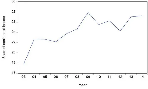
Firstly, Figure 1 shows the behavior of noninterest income in relation to the net operational revenue from 2003 to 2014.
Figure 1 Annual average evolution of from 2003 to 2014.
Source: Prepared by the author with Eviews 7.2 software with data from the Central Bank of Brazil’s database.
Correlation CAPITAL GROWTH
ASSET GDP HHIREV INTERESTREAL lnASSET SHLOAN SHNON PARTTIT PLCDATIVO CAPITAL 1.00000
GROWTHASSET -0.13409 1.00000
GDP 0.01882 0.04879 1.00000
HHIREV 0.42996 -0.02039 0.00614 1.00000
INTERESTREAL 0.02467 0.06994 0.18270 0.06437 1.00000
lnASSET -0.57590 0.04176 -0.03222 -0.50524 -0.16297 1.00000
SHLOAN -0.08064 0.06348 0.06141 0.24739 0.08236 -0.11953 1.00000
SHNON -0.19052 0.03974 -0.01038 -0.66474 -0.08242 0.20676 -0.33247 1.00000
SHTRD 0.19227 -0.03548 -0.03005 -0.16632 0.01967 0.02573 -0.30091 0.30181 1.00000
In line with Stiroh (2006) and Lepetit et al. (2008a), Figure 1 indicates that Brazilian banks behaved similarly to U.S. and European banks with regard to revenue diversification. In 2003, the average share of noninterest income in banks’ operating revenue was 17.8%. By 2014, the average SHNON was 27.4%. This suggests that bank revenue diversification also seems to be a trend for Brazilian banks, just as it is for financial institutions in other countries.
Before estimating the econometric models, we tested them for unit root problems using the method of Levin, Lin and Chu (2002), which provides a good indication. However, because it is not the most suitable test to be used with unbalanced panel data, we then conducted the following tests, which are the most suitable ones in this case: the Im, Pesaran and Shin, the ADF-Fisher Chi-square and the PP-Fisher Chi-square tests (Maddala & Wu, 1999; Hadri, 2000). All of these showed that the series are stationary at the 1% significance level. In addition, we conducted Kao and ADF panel cointegration tests for long-term equilibrium. Both tests showed that the series are cointegrated at the 1% significance level.
In order to check for the presence of clusters in the sample, which could originate significant heterogeneity, thereby causing problems in the panel data regression, an orthogonal factor model was estimated. Results showed no indication of significant cluster existence, i.e., the panel data regressions had no such problem.
Firstly, the models were estimated through OLS (Ordinary Least Squares), and we used the Hausman test to decide between fixed and random effects. Then, we tested for the presence of autocorrelation and heteroscedasticity, and results showed that all models had these problems.
Considering the problems above and the potential presence of endogeneity, mainly because the HHIREV,
SHNON, SHLOAN and SHTRD variables, we used an endogeneity test that was first proposed by Hausman (1978) and later improved by Davidson and MacKinnon (1989, 1993). All models had an endogeneity problem at the 1% significance level.
The presence of autocorrelation, heteroscedasticity and endogeneity led the estimation process towards the use of GMM, with a second step, cross sectional data differences and fixed effects for the periods, and Instrumental Variables (IV) estimators as defined by Arellano and Bond (1991). This method is based on the idea that instruments can estimate variables to mitigate endogeneity in models (Lee, Kim, Park & Sanidas, 2012).
The variables used as instruments are the lagged dependent variable, HHIREV and the period dummies. We used the lag number that optimized the J-statistic, whose null hypothesis is that the model is correct. This method generated estimations with correct instruments since all of them showed J-statistics p-values above 0.10 (Bhargava, 1991). In addition, we conducted the Arellano Bond serial correlation test, and found no evidence of second order serial correlation at the 10% significance level. The results of the econometric models are presented below.
Firstly, it is worth highlighting the relevance of the macroeconomic variables INTERESTREAL and GDP. Tables 3, 5 and 6 show that real interest rate is negatively related to σROA, positively related to ROAMEAN and negatively related to ZSCORE, respectively. All these results are significant at the 1% level. These results show that
INTERESTREALis related with a greater return; however, they are not clear about risk.
Table 3
Results of the σROA model
Variable Coefficient Prob.
σROA (-1) 0.175979 0.0000
INTERESTREAL -0.234101 0.0003
GDP -0.080143 0.5154
HHIREV -0.008772 0.3471
SHNON 0.009028 0.4868
SHLOAN 0.012574 0.0020
SHTRD 0.002321 0.2159
ACLASSET 0.294422 0.0000
lnASSET -0.010708 0.0016
GROWTHASSET 0.001636 0.3378
Variable Coefficient Prob.
PERIOD (2005) 0.004241 0.3920
PERIOD (2006) -0.003179 0.1316
PERIOD (2007) -0.004828 0.0680
PERIOD (2008) 0.003548 0.0256
PERIOD (2009) -0.014303 0.0020
PERIOD (2010) -0.009826 0.0486
PERIOD (2011) -0.006804 0.0004
PERIOD (2012) -0.014666 0.0000
PERIOD (2013) -0.008722 0.0002
PERIOD (2014) -0.008982 0.0888
Effects Specification
Mean dependent var -0.000464 S.D. dependent var 0.014102
S.E. of regression 0.016332 Sum squared resid 0.187781
J-statistic 54.92343 Instrument rank 75
Prob(J-statistic) 0.439408
Dependent Variable: σROA; Method: Panel Generalized Method of Moments; Transformation: First Differences; Date: 09/25/17 Time: 17:00; Sample (adjusted): 2005 2014; Periods included: 10; Cross-sections included: 111; Total panel (unbalanced) observations: 725; White period instrument weighting matrix; White period standard errors & covariance (d.f. corrected); Instrument specification: HHI_REV,-2; HHI_REV,-1; PERIOD; Constant added to instrument list.
Source: Prepared by the authors.
In addition, GDP also showed relevant results. Tables 5 and 6 show that GDP is positively related with ROAMEAN
and ZSCORE, respectively. These results are significant at the 5% and 1% levels, respectively. Therefore, these results confirm our expectation that the level of economic activity is related to more return and less insolvency risk for the banks analyzed.
As expected, SHNON showed a positive relationship with
RARROA and ROAMEAN at the 5% and 1% significance levels, according to Tables 4 and 5, respectively. These results are in line with Lee et al. (2014), and Sanya and Wolfe (2011) and corroborate hypotheses 1 and 3. Tables 3 and 6 did not show the expected signs for SHNON, but these results are not statistically significant. Moreover, results for SHNON are consistent about return and risk adjusted
return, but they are not clear about risk.
HHIREV showed a positive relationship with ROAMEAN, indicating that revenue specialization is positively related with return, as shown in Table 5. This result, significant at the 1% level, was not as expected. Our expectation was for a positive relationship between revenue diversification (not specialization) and return. However, further analysis of this result is necessary. In turn, if SHNON is found to be positively related with banks’ return, then it follows that specialization in noninterest income (rather than in interest income) is what drives results for HHIREV. Thus, results for HHIREV do not invalidate hypothesis 1; to the contrary, they corroborate it. In addition, Table 4 shows a positive relationship between HHIREV and risk adjusted return, which confirms hypothesis 3.
Table 4
Results of the RARROA model
Variable Coefficient Prob.
RARROA (-1) 0.303150 0.0000
INTERESTREAL -8.244321 0.1404
GDP 12.98872 0.1560
HHIREV 3.770102 0.0000
SHNON 1.814928 0.0398
SHLOAN 1.405083 0.0000
SHTRD 0.761438 0.0000
ACLASSET -15.62378 0.0027
lnASSET -0.010864 0.9587
GROWTHASSET -0.919211 0.0000
Table 3
Variable Coefficient Prob.
CAPITAL 1.488265 0.0599
PERIOD (2005) 1.024676 0.0003
PERIOD (2006) 0.839983 0.0000
PERIOD (2007) 0.220581 0.2691
PERIOD (2008) -1.681134 0.0000
PERIOD (2009) -0.236372 0.6918
PERIOD (2010) -0.144015 0.6121
PERIOD (2011) 0.706477 0.0042
PERIOD (2012) -0.594747 0.2795
PERIOD (2013) -0.575681 0.1250
PERIOD (2014) 1.338507 0.0175
Effects Specification
Mean dependent var -0.043482 S.D. dependent var 3.973193
S.E. of regression 4.576390 Sum squared resid 14744.11
J-statistic 91.56855 Instrument rank 110
Prob(J-statistic) 0.404942
Dependent Variable: RAR_ROA; Method: Panel Generalized Method of Moments; Transformation: First Differences; Date: 09/25/17 Time: 16:32; Sample (adjusted): 2005 2014; Periods included: 10; Cross-sections included: 111; Total panel (unbalanced) observations: 725; White period instrument weighting matrix; White period standard errors & covariance (d.f. corrected); Instrument specification: RAR_ROA,-2; HHI_REV, -1; PERIOD; Constant added to instrument list.
Source: Prepared by the authors.
Table 5
Results of the ROAMEAN model
Variable Coefficient Prob.
ROAMEAN (-1) 0.323124 0.0000
INTERESTREAL 0.389067 0.0000
GDP 0.112652 0.0204
HHIREV 0.063996 0.0000
SHNON 0.008486 0.0076
SHLOAN 0.007260 0.0000
SHTRD -0.001376 0.0283
ACLASSET -0.322270 0.0000
lnASSET -0.001951 0.0201
GROWTHASSET 0.029350 0.0000
CAPITAL -0.001982 0.4105
PERIOD (2005) 0.000240 0.9108
PERIOD (2006) 0.014485 0.0000
PERIOD (2007) 0.019600 0.0000
PERIOD (2008) 0.003747 0.0000
PERIOD (2009) 0.033849 0.0000
PERIOD (2010) 0.024067 0.0000
PERIOD (2011) 0.019376 0.0000
PERIOD (2012) 0.036366 0.0000
PERIOD (2013) 0.022605 0.0000
PERIOD (2014) 0.026455 0.0000
Effects Specification
Mean dependent var -0.001633 S.D. dependent var 0.022446
S.E. of regression 0.027134 Sum squared resid 0.531594
J-statistic 100.2280 Instrument rank 116
Prob(J-statistic) 0.336983
Dependent Variable: ROA_MEAN; Method: Panel Generalized Method of Moments; Transformation: First Differences; Date: 09/29/17 Time: 12:05; Sample (adjusted): 2005 2014; Periods included: 10; Cross-sections included: 119; Total panel (unbalanced) observations: 743; White period instrument weighting matrix; White period standard errors & covariance (d.f. corrected); Instrument specification: ROA_MEAN,-2; HHI_REV, -1; PERIOD; Constant added to instrument list.
Source: Prepared by the authors.
Table 4
Table 6
Results of the ZSCORE model
Dependent Variable: Z_SCORE; Method: Panel Generalized Method of Moments; Transformation: First Differences; Date: 09/29/17 Time: 12:13; Sample (adjusted): 2005 2014; Periods included: 10; Cross-sections included: 119; Total panel (unbalanced) observations: 743; White period instrument weighting matrix; White period standard errors & covariance (d.f. corrected); Instrument specification: Z_SCORE,-2; HHI_REV,-1; PERIOD; Constant added to instrument list.
Source: Prepared by the authors.
However, results for neither SHNON nor HHIREV were as expected with regard to risk, as shown in Tables 3 and 6. While results for SHNON were not statistically significant with regard to risk, HHIREV showed a positive relationship with ZSCORE, thus suggesting that revenue specialization is positively related with less insolvency risk. Although these results do not confirm hypothesis 2, they are in line with many empirical studies such as those by Stiroh (2006), Stiroh and Rumble (2006), DeYoung and Roland (2001), and Demsetz and Strahan (1997).
With regard to interest income, results for SHLOAN
showed a positive relationship with ROAMEAN and RARROA.
Both results presented a high statistical significance. In addition, a greater share of loan income in interest income is related with a greater risk, as measured by σROA. It is noteworthy that while the banks that are more specialized in traditional intermediation (loan) are more profitable, they also take greater risks than the ones that diversify their financial intermediation with trading or other income sources.
In turn, while SHTRD is negatively related with ROAMEAN, it showed a positive relationship with risk adjusted returns at the 5% and 1% significance levels. In addition, SHTRD
income is positively related with σROA, though not in a
Variable Coefficient Prob.
ZSCORE (-1) 0.224502 0.0000
INTERESTREAL -33.34173 0.0000
GDP 44.68439 0.0000
HHIREV 4.630959 0.0000
SHNON -0.354450 0.3377
SHLOAN 1.557418 0.0000
SHTRD -0.607977 0.0000
ACLASSET -29.94853 0.0000
lnASSET -1.156576 0.0000
GROWTHASSET 0.307556 0.0041
CAPITAL 29.60358 0.0000
PERIOD (2005) 1.811639 0.0000
PERIOD (2006) -0.092662 0.3408
PERIOD (2007) -1.103168 0.0000
PERIOD (2008) 0.570274 0.0001
PERIOD (2009) 1.238104 0.0000
PERIOD (2010) -1.717169 0.0000
PERIOD (2011) 0.596310 0.0000
PERIOD (2012) 0.121923 0.4565
PERIOD (2013) 0.511911 0.0000
PERIOD (2014) 2.355872 0.0000
Effects Specification
Mean dependent var -0.130649 S.D. dependent var 2.720231
S.E. of regression 2.093542 Sum squared resid 3164.467
J-statistic 94.19006 Instrument rank 116
statistically significant way, and negatively related with
ZSCORE at the 1% significance level. In general, banks with more diversified interest income sources, particularly with a greater share of trading activities, have lower returns than those whose interest income is concentrated on traditional loans. These results are in line with those of DeYoung and Roland (2001) and Mercieca et al. (2007), which similarly found a negative relationship between bank return and trading income.
ACASSET showed a positive relationship with risk and a negative relationship with both return and risk adjusted return at the 1% significance level. lnASSET was found to be negatively related with risk and return at the 1% and the 5% significance levels, as shown in tables 3 and 5, respectively.
GROWTHASSET showed a positive relationship with
ROAMEAN and a negative relationship with RARROA. Thus, having a growth strategy is related with a greater return for Brazilian banks, tough it is also related with a smaller
risk adjusted return. Some authors found similar results, such as Mercieca et al. (2007), Chiorazzo et al. (2008), and Lepetit et al. (2008a). However, this variable shows a positive relationship with ZSCORE, which indicates smaller bankruptcy risk.
CAPITAL showed a positive, statistically significant relationship with ZSCORE at the 1% level. This result suggests that banks with better capital levels have a greater capacity to reduce their bankruptcy risk. In addition, this variable presented a positive relationship with RARROA, suggesting that a better capital level positively affects the bank’s risk adjusted return.
Our main results suggest that the banks that chose to specialize in noninterest income tended to increase their return and risk adjusted return. As for banks that chose to specialize in interest income, our results suggest that traditional loan is positively related with a greater return and a smaller insolvency risk, while trading activities are related with a greater insolvency risk and a smaller return.
8 CONCLUSION
The present study aimed to determine the impact of revenue diversification on the risk and return of Brazilian banks. Results were relevant and added new evidence to the literature on the subject, which is still incipient in Brazil.
Firstly, a simple glance at Figure 1 shows the relevance of this theme to Brazilian banks. In 2003, noninterest income accounted for only 17.80% of the operating revenue of the banks analyzed. However, by 2014 this share had increased to 27.40%. Thus, income diversification has been a strategy that is present in Brazilian banks as well as in foreign banks, as described by Stiroh (2006) for U.S. banks and by Lepetit et al. (2008a) for European banks.
Hypothesis 1 was confirmed, according to the results in Table 5, with a positive relationship between
ROAMEAN and SHNON. If SHNON measures the direct effect of bank income diversification, then HHIREV measures the indirect effect. Thus, results for HHIREV which was found to be positively related to bank return, suggest that the concentration of income sources that would likely increase the banks’ return would be on the noninterest share.
The second hypothesis was not confirmed. SHNON
showed a positive (though not statistically relevant) relationship with risk. While it does not confirm hypothesis 2, this result is in line with many empirical studies such as those by Stiroh (2004), Stiroh (2006), Stiroh and Rumble (2006), DeYoung and Roland (2001), and Demsetz and Strahan (1997).
In turn, the positive relationship between HHIREV and
SHNON and risk adjusted return confirmed hypothesis 3. Both results presented statistical significance.
Among interest income sources, SHLOAN was found to be related with a greater return, while SHTRD presented a negative relationship with return and a negative relationship with ZSCORE, which means a greater risk. Therefore, in making a decision concerning interest income sources, results suggest that banks should choose loan activities rather than trading.
REFERENCES
Araújo, L. M. G., Gomes, G. M. R., Guerra, S. M., & Tabak, B. M. (2011). Comparação da Eficiência de Custo para BRICs e América Latina. [Working Paper]. Banco Central do Brasil.
Retrieved from http://www.bcb.gov.br/pec/wps/port/TD252. pdf.
Arellano, M., & Bond, S. (1991). Some tests of specification for panel data: Monte Carlo evidence and an application to employment equations. Review of Economic Studies, 58(1), 277-297.
Banco Central do Brasil (BACEN). SGS: Sistema Gerenciador de Series Temporais. Retrieved from https://www3.bcb.gov.br/ sgspub/localizarseries/localizarSeries.do?method=preparar TelaLocalizarSeries.
Berger, P. G., & Ofek, E. (1995). Diversification’s effect on firm value. Journal of Financial Economics, 37(1), 39–65. Bhargava, A. (1991). Identification and panel data models with
endogenous regressors. Review of Economic Studies, 58. Calmès, C., & Liu, Y. (2009). Financial structure change and
banking income: A Canada-U.S. comparison. Journal of International Financial Markets, Institutions and Money, 19(1), 128–139.
Chiorazzo, V., Milani, C., & Salvini, F. (2008). Income
diversification and bank performance: Evidence from Italian banks. Journal of Financial Services Research, 33(3), 181–203. Davidson, R., & MacKinnon, J. G. (1989). Testing for consistency
using artificial regressions. Econometric Theory, 5, 363–384. Davidson, R., & MacKinnon, J. G. (1993). Estimation and
inference in econometrics. Oxford University Press. De Jonghe, O. (2010). Back to the basics in banking? A
micro-analysis of banking system stability. Journal of Financial Intermediation, 19(3), 387–417.
De Paula, L. F., & Marques, M. B. L. (2006). Tendências Recentes da Consolidação Bancária no Brasil. Análise Econômica, 45, 235-263.
Demsetz, R. S., & Strahan, P. E. (1997). Diversification, Size, and Risk at Bank Holding Companies. Journal of Money, Credit and Banking, 29(3), 300–313.
Denis, D. J., Denis, D. K., & Sarin, A. (1997). Agency problems, equity ownership, and corporate diversification. Journal of Finance, 52(1), 135–160.
DeYoung, R., & Roland, K. P. (2001). Product Mix and Earnings Volatility at Commercial Banks: Evidence from a Degree of Total Leverage Model. Journal of Financial Intermediation,
10(1), 54–84.
Elsas, R., Hackethal, A., & Holzhäuser, M. (2010). The anatomy of bank diversification. Journal of Banking and Finance, 34(6), 1274–1287.
Gujarati, D. N., & Porter, D. (2011). Econometria básica. Porto Alegre: AMGH.
Hadri, K. (2000). Testing for Stationarity in Heterogeneous Panel Data, Econometric Journal, 3, 148–161.
Hausman, J. A. (1978). Specification tests in econometrics.
Econometrica, 46, 1251–1272.
Hayashi, F. (2000). Econometrics. New Jersey: Princeton University Press.
Laeven, L., & Levine, R. (2007). Is There a Diversification Discount in Financial Conglomerates? Journal of Financial Economics, 85, 331–367.
Lee, C. C., Hsieh, M. F., & Yang, S. J. (2014). The relationship between revenue diversification and bank performance: Do financial structures and financial reforms matter? Japan and the World Economy, 29, 18–35.
Lee, K., Kim, B.Y., Park, Y.Y., & Sanidas, E. (2012). Big businesses and economic growth: Identifying a binding constraint for growth with country panel analysis. Journal of Comparative Economics, 41, 561-582.
Lepetit, L., & Strobel, F. (2013). Bank insolvency risk and time-varying Z-score measures. Journal of International Financial Markets, Institutions and Money, 25(1), 73–87.
Lepetit, L., Nys, E., Rous, P., & Tarazi, A. (2008a). Bank income structure and risk: An empirical analysis of European banks.
Journal of Banking and Finance, 32(8), 1452–1467. Levin, A., Lin, C. F., & Chu, C. (2002). Unit Root Tests in Panel
Data: Asymptotic and Finite-Sample Properties. Journal of Econometrics, 108, 1–24.
Lin, J. R., Chung, H., Hsieh, M. H., & Wu, S. (2012). The determinants of interest margins and their effect on bank diversification: Evidence from Asian banks. Journal of Financial Stability, 8(2), 96–106.
Maddala, G. S., & Wu, S. (1999). A Comparative Study of Unit Root Tests with Panel Data and a New Simple Test. Oxford Bulletin of Economics and Statistics, 61, 631-652.
Markowitz, H. (1952). Portfolio Selection. The Journal of Finance, 1, 77-91.
Mercieca, S., Schaeck, K., & Wolfe, S. (2007). Small European banks: Benefits from diversification? Journal of Banking and Finance, 31(7), 1975–1998.
Navarro, P. S., & Procianoy, J. L. (1997). A reação dos acionistas à institucionalização do banco múltiplo. Revista de Administração, v.32, 68–79.
Sanya, S., & Wolfe, S. (2011). Can Banks in Emerging Economies Benefit from Revenue Diversification? Journal of Financial Services Research, 40(1), 79–101.
Stiroh, K. J. (2004). Diversification in Banking: Is Noninterest Income the Answer? Journal of Money, Credit, and Banking,
36(5), 853–882.
Stiroh, K. J. (2006). A Portfolio View of Banking with Interest and Norlinterest Activities. Journal of Money, Credit and Banking,
38(5), 1351–1361.
Stiroh, K. J., & Rumble, A. (2006). The dark side of diversification: The case of US financial holding companies. Journal of Banking and Finance, 30(8), 2131–2161.
Templeton, W. K., & Severiens, J. T. (1992). The effect of nonbank diversification on bank holding company risk. Quarterly Journal of Business and Economics, 4, 3–17.