FUNDAÇÃO GETÚLIO VARGAS
ESCOLA DE ADMINISTRAÇÃO DE EMPRESAS DE SÃO PAULO
JUNG CHIK PARK
BUSINESS CYCLE AND BANK LOAN PORTFOLIO PERFORMANCE:
EMPIRICAL EVIDENCE FROM BRAZILIAN BANKS
SÃO PAULO
JUNG CHIK PARK
BUSINESS CYCLE AND BANK LOAN PORTFOLIO PERFORMANCE:
EMPIRICAL EVIDENCE FROM BRAZILIAN BANKS
Dissertação apresentada à Escola de Administração de Empresas de São Paulo da Fundação Getúlio Vargas, como requisito parcial à obtenção do título de Mestre em Administração de Empresas.
Campo do conhecimento: Finanças
Orientador: Prof. Dr. Richard Saito
SÃO PAULO
Park, Jung Chik.
Business Cycle and Bank Loan Porfolio Performance: Empirical Evidence From Brazilian Banks / Jung Chik Park. - 2011.
51 f.
Orientador: Richard Saito.
Dissertação (MPA) - Escola de Administração de Empresas de São Paulo.
1. Bancos comerciais - Brasil. 2. Taxas de juros. 3. Empréstimo bancário - Brasil. 4. Desempenho. 5. Desenvolvimento econômico I. Saito, Richard. II. Dissertação (MPA) - Escola de Administração de Empresas de São Paulo. III. Título.
JUNG CHIK PARK
BUSINESS CYCLE AND BANK LOAN PORTFOLIO PERFORMANCE:
EMPIRICAL EVIDENCE FROM BRAZILIAN BANKS
Dissertação apresentada à Escola de Administração de Empresas de São Paulo da Fundação Getúlio Vargas, como requisito parcial à obtenção do título de Mestre em Administração de Empresas.
Data de Aprovação 13/12/2011
Membros da Banca:
Prof. Dr. Richard Saito FGV - EAESP
Prof. Dr. Rafael Schiozer FGV - EAESP
AGRADECIMENTOS
Gostaria de agradecer primeiramente a Deus e a todos que, direta ou indiretamente, contribuíram para a conclusão deste trabalho. Em especial, ao Prof. Dr. Richard Satio (EAESP/FGV) pela orientação acadêmica que permitiu a concretização desta dissertação.
Gostaria de agradecer ao Prof. Dr. Rafael Schiozer (EAESP/FGV) e ao Prof. Dr. Rogério Sobreiro (EBAPE/FGV) pela participação na banca examinadora e também pelas críticas e sugestões que contribuiram para o enriquecimento deste trabalho.
A todos os meus professores da EAESP/FGV, meu profundo agradecimento pelo ensino e a contribuição à minha formação acadêmica.
À Prof. Dra. Marina Heck, coordenadora do curso, e aos funcionarios da secretaria e biblioteca, meus sinceros agradecimentos por toda a orientação e apoio nestes anos.
Aos meus colegas da turma de mestrado pelo apoio nos momentos de sufoco e pela descontração que passamos juntos.
Especial agradecimento ao meu amigo Vinicius Augusto Brunassi Silva, aluno da EAESP/FGV, pelas conversas e apoio para realização desta dissertação.
Aos meus pais, Myung Wha Park e Eh Ja Park Chang, e aos meus irmãos, John Park e Daniel H. C. Park, por todo o suporte à minha formação acadêmica e amor durante toda a minha vida.
Especial agradecimento à Daniele C. Morales, minha esposa e companheira, que sempre me incentivou e esteve ao meu lado em todos os momentos com todo o seu amor e carinho.
INDEX
1. Introduction 1
2. Theoretical Reference 3
2.1. History of the Relation between the Economic Activity and the Financial
System 3
2.2. Macroeconomic determinants in the performance of the credit portfolio 4
2.3. Economic Growth Determinants 6
2.4. Loan interest rate determinants 7
2.5. Credit Risk, Determinants and Regulation 8
3. Methodology 13
3.1 Data Source 13
3.2. Empirical Model 15
4. Results and Analyses 23
4.1 Robustness Test 34
5. Conclusion 36
TABLES LIST
Table 1 – Provision per Risk Level 10
Table 2 – Number of Banks per Quarter 13
Table 3 – Credit portfolio per type of bank 14
Table 4 – Descriptive Statistic on the Explanatory Variables 22
Table 5 – Provision to Non-Performing Loans (NPL) Regressions on
Quarterly Lags of GDP and of Interest Rates, as well as other banking
system characteristics 24
Table 6 – Provision to Non-Performing Loans (NPL) Regressions on
Two-Quarter Lags of GDP and of Interest Rates, as well as other banking
system characteristics 26
Table 7 – Provision to Non-Performing Loans (NPL) Regressions on
Two-Quarter Lags of GDP and Interest Rate 29
Table 8 – Hausman Test 31
Table 9 – Results of 2SLS regression 32
APPENDIX
ABSTRACT
This paper studies the effects of economic growth and interest rates on the performance of Brazilian commercial bank loan portfolios in the period 2000 to 2010.
The results provide empirical evidence that economic growth is the main "driver" for performance of the loan portfolio. No evidence has found on the interest rate variation on NPL.
Moreover, there is empirical evidence that performance reasoned by GDP is lagged by 2 quarters.
Furthermore, the results show that the GDP variations correlated significantly with the performance level variations of Brazilian commercial banks, with a two-quarter lag throughout the period of one year.
Finally, the results show that changes in GDP most significantly impact on the performance of the largest Brazilian commercial banks’ loan portfolio. Due to the
multiplier effect of the credit market, the bigger the bank, the higher the relative expansion of its loan portfolio, and the higher its non-performing loan, which is aggravated by the credit market concentration in Brazil.
RESUMO
Este trabalho estuda os efeitos do crescimento econômico e da taxas de juros sobre
o desempenho de carteiras de empréstimo dos bancos comerciais brasileiros no
período de 2000 a 2010.
Os resultados empíricos mostram que o crescimento econômico é o principal "driver"
para o desempenho da carteira de crédito. Não foram encontradas evidências
estatísticas sginificativas de mudanças na taxa de juros sobre o desempenho das
carteiras de empréstimos.
Além disso, há evidências empíricas de que o impacto do crescimento econômico
sobre o desempenho da carteria de crédito tem efeito defasado de 2 trimestres.
Por fim, os resultados mostram que alterações de PIB impactam de forma mais
significativa o desempenho da carteira de crédito dos bancos comerciais brasileiros
maiores. Devido ao efeito multiplicador do mercado de crédito, quanto maior o
banco, maior a expansão relativa de sua carteira de crédito e, conseqüentemente a
taxa de inadimplência da carteira, que é agravada pela concentração do mercado de
crédito no Brasil.
Palavras-chave: crescimento econômico (PIB), taxa de juros, desempenho da
1 1. INTRODUCTION
The global financial crisis experienced by loan granting institutions worldwide during the 2008-2009 time periods renewed the interest in understanding the performance of banks during the business cycle. In a global economy, developing countries have been steadily increasing their importance as evidenced by the emerging market crises of the 1990s. This has brought up a heightened level of concern expressed by regulators, analysts and investors regarding the overall strength of the banking system not only amongst the developed countries, but also, and more importantly, in the developing world.
In most modern banking systems, transactions involving the lending and issuance of credits are some of the primary activities that can potentially expose lending institutions to risks of loss. Credit risk can be defined as the risk of loss of principal or loss of a financial reward stemming from a borrower’s failure to repay a loan or
otherwise meet their contractual obligation. Credit risk also arises whenever a
borrower’s credit quality deteriorates and is expecting to use future cash flows to pay
a current debt. Even though this does not result in an immediate loss of principal for the lending institution, there is a greater probability that a default will occur and this closely ties the risk to the potential return on an investment. Another notable instance being that the yields of bonds correlate strongly to their perceived credit risk. (Basel Committee on Banking Supervision, 1998).
Credit risk is affected by the likelihood of a potential borrower defaulting on his or her
financial obligations with a lending institution. Thus, the quality of a bank’s loan
portfolio is mainly determined by the rate of defaults. Credit risk management must
be the lending institution’s primary line of defence in order to prevent transactions
that will give credit to customers who will fail to meet the terms of the loans. Credit
risk management is an important aspect of a bank’s success and ensures that the lending institution will not take on undue risk.
2
turn, can have a significant impact on the rate of an economic expansion or recession. (Bernanke et al., 1998).
Despite a great deal of research on these macroeconomic determinants impact the immediate performance of banks, there are only a few studies which relate the performance of Brazilian banks and our macroeconomic environment, particularly when critical periods are factored into consideration.
In order to further contribute to our understanding of this relationship, this paper tested the effects of economic growth (GDP), as well as the changes in interest rate on the performance of Brazilian commercial bank loan portfolios from 2000 through 2010, taking into account the assessment model used by Glen and Velez (2010).
The empirical result showed that there is a strong correlation between economic growth (GDP) and the performance of the loan portfolios from Brazilian commercial lending institutions, while the variation in the interest rate has had no significant statistical effect. Furthermore, there is empirical evidence suggesting that the impact of the economic growth on the performance of the credit portfolio may not be immediate. In fact, it has historically taken an average of two quarters for the effect to be produced.
Finally, the results showed that changes in GDP most significantly impact on the performance of the largest Brazilian commercial banks’ loan portfolio. Due to the
multiplier effect of the credit market, the bigger the bank, the higher the relative expansion of its loan portfolio, and the higher its non-performing loan, which is aggravated by the credit market concentration in Brazil.
This paper is organized in the following way: section 2 presents the theoretical references; section 3 presents the utilized data, the sample selection, the empirical model, and the descriptive statistics; section 4 presents the results and discussions; and section 5 presents the conclusion of this paper.
3 2. THEORETICAL REFERENCE
2.1 History of the relation between the economic activity and the financial system
The relationship between the economic activity and the overall health of the financial system has become more clearly understood by economists due to advancements in macroeconomic theories.
According to Keynes (1936), the level of economic activity was determined by the level of aggregate demand. Additionally, he argued that capitalist economies were subject to periodic weakness in the aggregate demand generation process, resulting in unemployment.
In 1933, Fisher demonstrated that one of the main contributing factors to the severity of the Great Depression in 1929 was the ill preparedness of the financial markets at the time. The author introduced the concept of debt deflation in order to explain that the deflation of prices actually increased people’s real indebtedness. This, in turn,
caused them to cut down on their expenses and investments causing even further deflation, and, consequently, promoting a vicious cycle that inevitably lead to the instability in the world's economy. Also, in 1963, Friedman and Schwartz presented a strong positive correlation between monetary offers and production of goods, especially during the Great Depression, underscoring how pivotal the role of lending institutions is because they mobilize the currency across the financial market. Likewise, understanding their importance in the financial system is crucial to the
recovery of the world’s economy.
Furthermore, Bernanke’s studies (1983) concluded that the banking crisis was
4
economic cycle had a significant impact on consumers’ expenses, using data from the crisis of 1929.
Akerlof’s studies in 1970 highlighted the imperfections in the credit market and their implications for the financial market at the microeconomic level, such as the imbalance of information and critical problems within the agency itself. According to Bernanke et al.(1998), the lack of consistency of information has an important role in the relation between creditors and debtors; concluding that the contracts, the monitoring cost and incentive policies all interfere in the credit market. Thus, the author presents a macroeconomic model which incorporates both the imbalanced information and the agency cost in loan relations, impacting on cycles of economic activity.
However, according to Gertler (1988), the macroeconomic literature which followed the publication of the General Theory practically ignored the potential link between the economic activity and the performance of the credit market.
In Brazil, research in this area started essentially during the early 1990's, fundamentally analysing the implications over the economic growth originated in the public infrastructure with the pioneering studies by Ferreira (1996), Garcia (1996), Ferreira and Malliagros (1998), and Rigolon (1998).
Specifically, where the role of the financial system in the process of the economic growth in Brazil is concerned, Gonçalves (1980) and Studart's (1993) contributions can be marked off. Arraes and Teles (2000) examined the productive issue with secondary focus over the credit role offered by the financial system, and Triner (1996)
2.2 Macroeconomic determinants in the performance of the credit portfolio
This section presents studies accomplished about macroeconomic determinants in
5
In 2001, Chu investigated the main macroeconomic factors that helped explain banking default during the period from 1994 to 2000. The author inferred that the GDP, the Spread (difference between application rate and funding rate), Interest
Rate and Unemployment are, respectively, the factors that Brazilian banks’
expenditures and default are most sensitive to.
Takeda, in 2003, evaluated the effects of monetary policy on credit offer and concluded that the Central Bank Compulsory Deposits Rate (remunerated deposits) is one of the instruments of monetary policy, and he also demonstrated that there is a positive correlation between credit offer and the industrial GDP.
In 2003, Pain investigated the factors which explain the increase in loan loss provision amongst the eleven biggest UK banks. The result showed that macroeconomic factors, such as the Gross Domestic Product (GDP), the real interest rate, and loan portfolios, as well as specific factors, such as loans to certain segments of the economy, are associated with provision levels.
Motivated by the Greek financial crisis, Louzis, Vouldis and Metaxas carried out a study in 2010 that shows that the performance of Greek banks' loan portfolios can be explained mainly by the GDP, real interest rate, and employment rate, apart from the managerial quality of financial institutions.
Most recently, in 2010, Glen and Velez studied the effects of the GDP and the real
interest rate upon the performance of commercial banks’ credit portfolios from
6 2.3 Economic Growth Determinants
Gonzaga et al.(1995) studied the relevance of permanent shocks in the explanation of the product variance in typical periods of economic cycles. The author concluded that transitory shocks to the product are practically irrelevant when compared to the permanent ones. The author shows that anticyclical economic policies, which control transitory shocks (e.g.: monetary policies of added demand control), have extremely limited effectiveness, and that, given the importance of permanent shocks, it is necessary that economic determinants of long-term shocks over the product be investigated. The authors also researched the long-term effects of education, foreign investments, and economic growth. The authors inferred that, except for illiteracy rate, the tested series had a long-term relationship with the Brazilian prospective product.
In 1995, Fava and Cati investigated the reasons behind the trends found in the Brazilian gross domestic product, either stochastic or deterministic, by using the GDP series referring to data from 1900 through 1993. Based on the Dickey-Fuller unit root test and on the unit root tests proposed by Perron (1989 and 1993), the Additive Outlier Model (AO) and the Innovational Outlier Model (IO), they found evidence that Brazilian GDP did not have a stochastic tendency until 1980. The period during which the tendency was first observed coincided with economic crisis in the early 1980's.
According to Cardoso (1997), there are basically four factors which account for the economic growth in leading countries: The accumulation of physical capital; the accumulation of human capital; the accumulation of technology; and, the operation standards of the country’s institutions.
7
capital, and working factors, by the externalities which lead to bigger marginal productivities, by the long-term economic stability, by education, and by investments in human capital. In the short term, however, changes in the GDP are related to interest rates, currency control, and fiscal policies.
In 2003, based on Solow’s economic growth model, Tonini evaluated the effects of
the investment levels in education as well as the effects of physical capital storage on Brazilian economic growth, from 1975 through 2000. The author suggests that the investments in these two variables were low, which confirmed the low level of growth
in Brazilian economy, especially in the 1980’s.
2.4 Loan interest rate determinants
According to HO and SAUNDERS (1981), an elevation in the basic interest rate causes not only the market interest rates to increase, but also an increase in banking interest rates.
In 1989 Berger and Hannan proposed that the banking concentration has a considerable impact on the interest rates due to the fact that a more concentrated banking sector tends to act oligopolistically, thus, charging higher interest rates.
Research by Kashvap and Stein in 2000 concluded that smaller banks, particularly ones with low liquidity and capitalization, charge higher loan interest rates because investors charge higher bonuses due to the risk.
In Brazil, Koyama and Nakane (2002) evaluated the determinants of “banking
spread”, inferring that the most relevant component is related to the risk perception, which is related to the macroeconomic environment scenario of the country, mainly due to perspectives of economic growth.
8
banks, allowing them to loan more. Besides, the author enhances the fact that banking costs, along with resource funding, monitoring, maintenance of bank agencies, among others, also affect loan rates for such costs partly reflect on the level of banks' efficiency.
2.5 Credit Risk, Determinants and Regulation
Altman (1968) argued that the development of a new predictive model was necessary due to the growth in bankruptcies as well as the organizations' financial changes, aggravated by the drastic increase of the average size of bankrupted companies.
In 1974, The Basel Committee was formed by central banks of countries which comprised the Group of Ten (G-10): Belgium, Canada, France, Germany, Italy, Japan, the Netherlands, Sweden, Switzerland, the United Kingdom, and the United
States, after the bankruptcy of Herstatt Bank. The committee’s decisions had neither
legal power nor supranational supervising authority. Nevertheless, such decisions were widely accepted for they estimated the convergence of banking supervision techniques of the member countries to common standards and approaches, which made feasible the capital flow among countries without imposing barriers, as well as guaranteed the safety of such capitals.
In 1988, the Basel Accord, or Basel I, was signed and ratified by over 100 countries. This accord aimed to create minimum requirements of capital capital, which must be complied with by commercial banks, preventively against credit risk. Since then, capital requirement has been based on risk, establishing that the minimum capital requirements must comply with the economic loss anticipations of each financial institution.
Berger and Deyoung, in 1997, assumed that default credits can be caused by
exogenous components, such as economy deceleration and companies’
bankruptcies. On the other hand, the authors enhance the possibility of managerial
inefficiency, an endogenous component, caused by managers’ inefficient
9
According to Bessis (1998), the credit risk can be defined by losses begotten by a
debtor’s default event or by the deterioration of its credit quality. The author stated that the deterioration of the debtor’s credit quality does not result in an immediate
loss for the financial institution, but in the increase of the probability that a default event happens. Thus, the credit risk can be evaluated from its components, which comprise the default risk, the exposure risk, and the recovery risk.
According to Caouetteet al.(2000), credit generally involves the expectation of receiving a value in a certain period of time. In this sense, the author stated that the credit risk is the chance such an expectation will not be lived up to.
Houaiss (2001) defined the word “default” as: “[...] lack of complying with an obligation". Westgaard and Wijst (2001) stated that: “[...] defaulting is failing in paying
an amount of money owed to a bank”. Bessis (1998) presents the following definitions: “[...] neglecting to pay an obligation, breaking an agreement, starting a
legal procedure or an economic default”.
A wider definition was adopted by The Basel Committee on Banking Supervision (BCBS) in 2004: A default is regarded to have happened in relation to a specific debtor when one or both of the following events have occurred:
The bank regards as improbable that the debtor pays the total amount of its
obligations to the financial conglomerate without actions such as having the debtor give it guarantees (if possessed);
The debtor is overdue for over 90 days regarding some material obligation with the financial institution.
According to Sicsú (2003), it is difficult to reach a consensus among credit analysts when it comes to an operational definition of default for the analysts' objectives can be conflicting. Some tend to adopt more rigorous criteria aiming to obtain a risk classification system which approves of credit operations more parsimoniously.
However, other analysts, concerned with the creation of a system that limits banks’
10
In 2009, Filippaki and Mamatzakis highlighted that bank managers oppose to risk so much that they could increase operational expenditures on loan assessments and monitoring, which reduces efficiency, in order to cut down default participation in their credit portfolios.
In Brazil, the biggest adjustment was due to the introduction of Resolution CMN nº 2682 from 12/21/1999, which establishes the classification criteria of credit operations for the constitution of loan loss provision (LLP).Such Resolution obliges banks to develop consistent credit models that allow the determined classification there under, according to table 1.
Table 1 – Provision per Risk Level
Risk level Provision
AA 0.00%
A 0.50%
B 1.00%
C 3.00%
D 10.00%
E 30.00%
F 50.00%
G 70.00%
H 100.00%
Source: Resolution 2682/99, Banco Central do Brasil
According to the Resolution, the operation classification at risk levels must be reviewed, at least on a monthly basis, on the occasion of financial statement report, due to verified overdue payment of principal amount installments or charges installments, in compliance with the following:
11
e) 121 to 150 days overdue: level F risk, at least; f) 151 to 180 days overdue: level G risk, at least; g) overdue for more than 180 days: Level H risk;
According to Parente (2000), Resolution 2682/99, published to substitute Resolution 1748/90, has characteristics that dissociate it, in many aspects, from the provisioning rules forecast in its precedent. Thus, it came up to comply with the necessity of more rigor in such rules and of an adequacy of Brazilian norms to international standards.
Jorion (2003) highlighted that banking regulation is necessary to extinguish the effects caused by a probable mismanagement of the institution’s resources, which
puts its creditors and stockholders at risk.
According to Andrade (2003), credit risk models can be classified in three groups: risk classification models, stochastic models of credit risk and portfolio risk models. Risk classification models seek to assess either a debtor's risk or an operation risk, giving it a measure that represents the default risk expectation, generally expressed as a risk classification (rating) or score. Risk classification models are used by financial institutions in their credit award processes.
Schechtman et al. (2004) and Schechtman (2006) analyzed the adequacy of
provision levels and regulating capital required by Brazil’s Central Bank (Bacen) and infer that such levels are sufficiently robust to cover Brazilian financial institutions’
credit risk exposure.
In 2008, Chang et al. presented evidence that approximately 10% of the banks of the domestic financial system account for practically the totality of loans in the banking market. In 2009, Tecles, Tabak, and Staub analyzed the loan market in Brazil from 2003 through 2008 to measure the diversification as well as the default
12 Due to many bankruptcies of financial institutions in the 90’s, in 2004, the Basel Committee launched a new document which substituted the 1988 Accord, named Basel II Capital Accord Basileia II, which is fixed on three pillars and 25 basic principles about accounting and banking supervision. According to BACEN (2004), Basel II Accord is an evolution of the one signed in 1988, which is underway in the Committee on bank monitoring. The new structure intends to improve itself by emphasizing the administration and the own control of banks in the managerial process of review and in the market discipline.
13
3. METHODOLOGY
This section presents the data sources used in this paper, the empirical model, the dependent variables, the explanatory variables, the control variables, and the descriptive statistics.
3.1 Data Source
The financial data present herein were directly obtained from Banco Central do
Brasil’s website. The author used quarterly data from all accounting positions of banking institutions such as Bank Conglomerate and Independent Banking Institutions like Commercial Bank, Multiple Bank with Commercial Portfolio or Thrift
and Savings Bank, which had credit portfolio, according to Central Bank’s
classification.
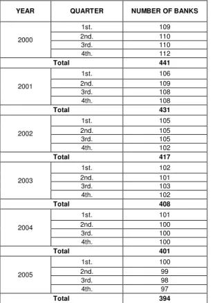
Financial data from banks were collected ranging from 2000 through 2010, with base date at the end of every quarter of the respective years, according to table 2.
Table 2 – Number of Banks per Quarter
YEAR QUARTER NUMBER OF BANKS
2000
1st. 109
2nd. 110
3rd. 110
4th. 112
Total 441
2001
1st. 106
2nd. 109
3rd. 108
4th. 108
Total 431
2002
1st. 105
2nd. 105
3rd. 105
4th. 102
Total 417
2003
1st. 102
2nd. 101
3rd. 103
4th. 102
Total 408
2004
1st. 101
2nd. 100
3rd. 100
4th. 100
Total 401
2005
1st. 100
2nd. 99
3rd. 98
4th. 97
Total 394
YEAR QUARTER NUMBER OF BANKS
2006
1st. 97
2nd. 97
3rd. 96
4th. 95
Total 385
2007
1st. 95
2nd. 94
3rd. 93
4th. 93
Total 375
2008
1st. 93
2nd. 93
3rd. 95
4th. 95
Total 376
2009
1st. 93
2nd. 94
3rd. 94
4th. 94
Total 375
2010
1st. 93
2nd. 92
3rd. 93
4th. 93
Total 371
General Total 4374
14
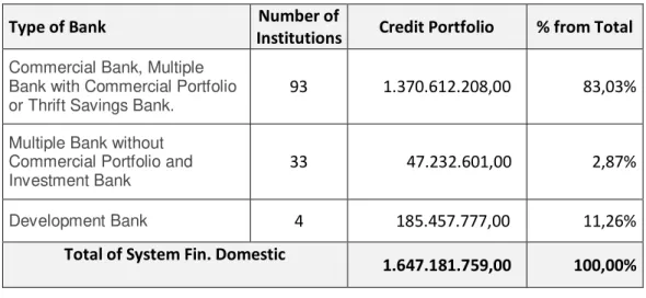
On the base date 12/31/2010, the credit portfolio (credit operations and leasing) of the 93 banks totalized BRL 1.37 trillion out of BRL 1.65 trillion from the total Domestic Financial System, that is, 83.03%. Non-participants in this study: credit cooperatives, non-banking institutions, banks without commercial portfolio, investment banks, and development banks, according to table 3.
Table 3 – Credit portfolio per type of bank
BRL Thousands
Type of Bank Number of
Institutions Credit Portfolio % from Total Commercial Bank, Multiple
Bank with Commercial Portfolio
or Thrift Savings Bank. 93 1.370.612.208,00 83,03%
Multiple Bank without Commercial Portfolio and
Investment Bank 33 47.232.601,00 2,87%
Development Bank 4 185.457.777,00 11,26%
Total of System Fin. Domestic
1.647.181.759,00 100,00%
Source: Banco Central do Brasil (12/31/2010)
On 12/31/2000, the 5 largest commercial banks represented together 79% of the total commercial bank portfolio (USD 1.08 trillion), according to the graphic below:
15 3.2 Empirical Model
The empirical analysis of this paper was carried out by means of using panel econometrics with estimation per fixed effects. The decision to use this method was
based on Hausman’s test, in which the possibility of the non-existence of correlation between the non-observable effect and the explanatory variables throughout the whole period of the sample was rejected, thus eliminating the possibility of random effects estimation. Tests were done by considering, also, correction for heteroscedasticity.
Firstly, data referring to performance (NPL– non-performing loan, used as dependent
variable), GDP and Interest Rate (central independent variables in the analysis), and other control explanatory variables (as presented in the following section) were groups by quarters from 2000 through 2010, with the sample organization in cross-sectional dimension.
Thus, according to Glen and Velez (2010), there is the following empirical model to be tested:
𝑁 𝑎 𝐿 𝑎 𝑁𝑃𝐿 𝑖, = 𝛽0𝑖, + 𝛽1𝐺 𝑃𝑖, +𝛽2𝐺 𝑃𝑖, −1 + 𝛽3𝐺 𝑃𝑖, − 2 +⋯+ 𝛽4𝐺 𝑃𝑖, −n +𝛽5𝛥𝐼 𝑅𝑎 𝑖, +𝛽6𝑅 𝑎 𝐼 𝑅𝑎 𝑖, −1 +
𝛽7𝑅 𝑎 𝐼 𝑅𝑎 𝑖, −2 +⋯+𝛽8𝑅 𝑎 𝐼 𝑅𝑎 𝑖, −n +𝛽9 𝐴 𝑖 𝑦 𝑖, +
𝛽10 𝑖𝐴𝑃 𝑖 𝑖, +𝛽11 𝑖, +ℯ
Where:
NPL𝑖, : ratio of the loan loss provision, according to Resolution 2682/99 of Bacen, to net loan portfolio for bank i at time t.
GDP 𝑖, : Variation of gross domestic product in the quarter compared to the
same quarter of the previous year for bank i at time t.
16 GDP 𝑖,t-2: Variation of gross domestic product in two previous quarters
compared to the respective quarter of the previous year for bank i at time t-2.
GDP 𝑖, -n: Variation of gross domestic product in “n” previous quarters compared to the respective quarter of the previous year for bank i at time t-n.
Δ Interest Rate𝑖, : Variation of interest rate of the quarter related to the previous one for bank i at time t.
Real Interest Rate𝑖, -1: Real interest rate, that is, by deducting inflation of the period for bank i at time t-1.
Real Interest Rate 𝑖, -2: Real interest rate, that is, by deducting inflation two period for bank i at time t-2.
Real Interest Rate 𝑖, -n: Real interest rate of “n” previous period, that is, by deducting inflation of the respective period for bank i at time t-n.
Equity/ Assets𝑖, : Total of Equity divided by Assets for bank i at time t.
Credit Portfolio/Assets𝑖, : Total of Credit Portfolio divided by Assets for bank i
at time t.
CD𝑖, : Control dummy of crisis period for bank i at time t.
The hypothesis, based on the results from the work by Glen and Velez (2010), is that the explanatory variable, GDP, has a significantly negative relation with the credit portfolio performance, while the interest rate has a positive relation. So, there are:
H1: Negative and significant relation between GDP and NPL
H2: Positive relation of the variation between interest rate and NPL
The dependent variable NPL (Nonperforming Loan) of the credit portfolio is the ratio of the loan loss provision, according to Resolution 2682/99 from Bacen, to net loan portfolio at a certain time. High default levels result in higher provisions; thus, default reserves can be regarded as a quality tool of the bank's credit portfolio.
17
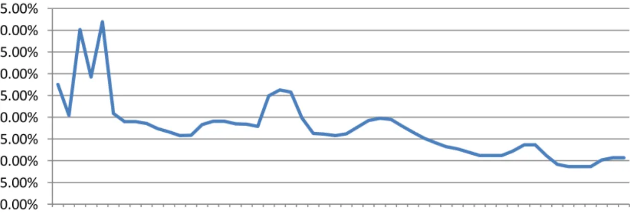
Graphic 1- Evolution of the NPL rate
Source: Banco Central do Brasil
It is noticeable that the NPL rate decreased throughout the 3rd quarter of 2000, down
from 9% to 5.98% in the 4th quarter of 2001. In 2002 and 2003, the NPL returned to
its 9% level. From 2005 through 2008, the NPL rate kept decreasing until it reached around 4.10% in the 2nd quarter of 2008. In the 3rd quarter of 2009, an elevation of the NPL rate to 7.5% had occurred. In 2010, the rate returned to its low tendency, closing the year at 4.28%.
The gross domestic product (GDP) represents the sum (in monetary values) of all final goods and services produced in a certain region whether it is a country, a State, or a city), during a certain time (month, quarter, year, etc). The GDP is one of the most commonly used indicators in macroeconomics, and aims to measure the economic activity of a region.
There are two calculations of the GDP, one nominal and another one real. The former refers to the value of the GDP calculated at current prices, that is, in the year when the product was made and traded. The latter is calculated at steady prices, in which a base year is chosen so as to do the calculation of the GDP, eliminating, then, the inflation effect. For more consistent assessments, the Real Quarterly GDP was used, which is the comparison between the real GDP of the quarter to the real GDP of the equivalent quarter in the previous year. Graphic 2 presents the evolution of
18
Graphic 2 – Evolution of real GDP (% per quarter)
Source: IBGE
It is noticeable an increase in the GDP in 2000 and a plunge in 2001. The same occurred in 2002-2003. From 2003 on, there was a strong increase in the economic growth, reaching 7.10% in the 3rd quarter of 2008. In 2009, it is noticed a downturn in
the economy, plummeting -2.98% in the 3rd quarter. In 2010, there is an accentuated
recovery of Brazilian economic activity, rocketing 9.3% in the 1st quarter.
An explanation for the bad performance in 2009 would be the drops in the industrial production volumes, as well as the strong reduction of investments, from respectively 5.5% and 9.9%, due to the global subprime crisis triggered in September, 2008.
Graphic 3 shows the evolution of the relation between the total bank loans and the real GDP from 2000 to 2010.
19
Graphic 3 – Volume of Credit Portfolio over the real GDP
Source: Banco Central do Brasil
It is noticed from 2005 an increase in the relation between the volume of bank loans and the GDP, rocketing from 25% to 45% in 2010, being the credit volume in the country the highest since the beginning of the Brazilian Real Plan.
According to Bacen, the Selic rate is obtained through the calculation of the weighted average rate and adjusted from the one-day financing operations, spread in federal public bonds and passed in either the referred system or in compensation chambers and assets liquidation as buyback transactions. From the content present, it can be inferred that the Selic rate is originated from the interest rate effectively observed in the market.
Graphic 4 presents the variation of the interest rate from 2000 through 2010.
Graphic 4 – Variation of Interest Rate (% per year)
Source: Banco Central do Brasil
10% 15% 20% 25% 30% 35% 40% 45% 50%
2000 2001 2002 2003 2004 2005 2006 2007 2008 2009 2010
20
Since 2002, the interest rates have been decreasing gradually from 25% per year to the level of 10% per year in 2009/2010.
Based on J. Glen and Velez C. M.'s research (2010), the control variables tested in this paper are:
The relation between the loan portfolio and banks' assets. Graphic 5 presents the
evolution of this relation from 2000 through 2010.
Graphic 5 – Total of Credit Portfolio over Total of Assets
Source: Banco Central do Brasil
It can be noticed that the relation between the volume of the credit portfolio and assets remained stable, between 35% and 37% in the period.
Equity over banks’ assets suggests that a bigger capitalization of banks is a
“barrier” against cyclic effects. Graphic 6 presents the relation between Equity over Brazilian banks' assets from 2000 through 2010.
10.00% 15.00% 20.00% 25.00% 30.00% 35.00% 40.00%
21
Graphic 6 – Total of Equity over Total Assets
Source: Banco Central do Brasil
Through the observed period, the relation between Equity and Assets remained stable throughout the period, at approximately 25%.
Crisis Period. Crisis dummies will be inserted in order to check features of specific periods of crisis. Crisis periods were regarded as: second half of 2001 (terrorist
attempt on 09/11/2001); the year 2002 (Lula’s presidential election); second half
of 2008, and the year 2009 (subprime crisis).
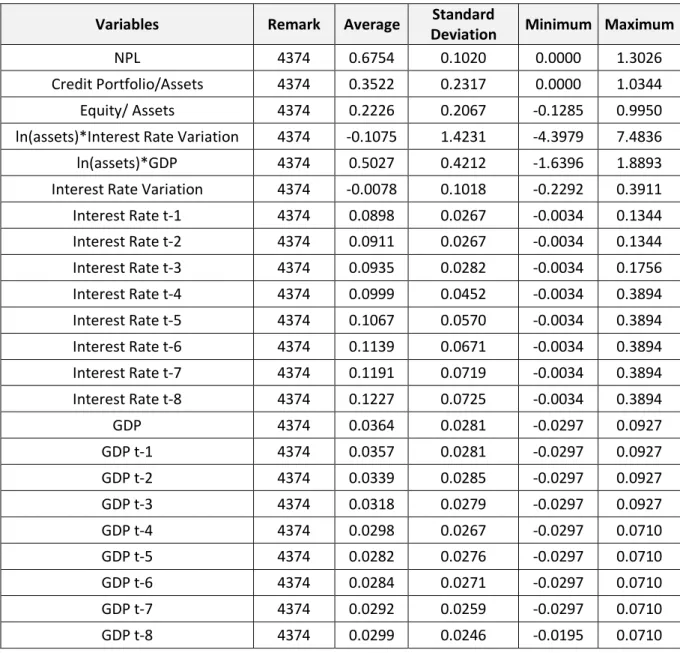
Table 4 presents the descriptive statistic of the explanatory variables used in the study of the relations between performance of the credit portfolio (NPL), the interest rate, and the economic growth (GDP). All the data are consolidated and include those from the parent company and its controlled undertaking. The analyzed period was 2000 through 2010.
The correlation matrix between variables lies in appendix.
0.00% 5.00% 10.00% 15.00% 20.00% 25.00% 30.00%
22
Table 4 – Descriptive Statistic on the Explanatory Variables
The credit portfolio corresponds to the totality of credit operations and commercial leasing. The loan loss provision was determined based on the information provided by Banco Central do Brasil (Central Bank of Brazil), which determines provisioning percentages of credit operations (LLP) according to their overdue periods, as in Resolution CMN 2682/99. The NPL (performance) of the credit portfolio is given by dividing the LLP by the total amount of the credit portfolio. The interest rate corresponds to the Selic rate of the equivalent year, that is, the basic interest rate used as a reference by the monetary policy. The variation in the interest rate equivalent to the percentage level of the change in the Selic interest rate related to the previous quarter. The interest rate t-n is the Selic interest rate done in “n” previous quarter. The GDP corresponds to the quarterly growth rate of the sum (in monetary values) of all goods and services produced in the country throughout the period compared to the equivalent quarter of the previous year. GDP t-n corresponds to the economic growth rate noticed in “n” previous quarter. The
bank’s loan level (Credit Portfolio/Assets is given by the relation between the credit portfolio and its total assets. The level of assets financing per own capital (Equity/ Assets) is given by the relation between Equity and Assets of each financial institution. Ln(assests)* Delta Interest Rate is the natural log of assets of each financial institution multiplied by interest rate variation. Ln(assets)*GDP is the natural log of assets of each financial institution multiplied by the quarterly economic growth rate.
Variables Remark Average Standard
Deviation Minimum Maximum
NPL 4374 0.6754 0.1020 0.0000 1.3026
Credit Portfolio/Assets 4374 0.3522 0.2317 0.0000 1.0344
Equity/ Assets 4374 0.2226 0.2067 -0.1285 0.9950
ln(assets)*Interest Rate Variation 4374 -0.1075 1.4231 -4.3979 7.4836
ln(assets)*GDP 4374 0.5027 0.4212 -1.6396 1.8893
Interest Rate Variation 4374 -0.0078 0.1018 -0.2292 0.3911
Interest Rate t-1 4374 0.0898 0.0267 -0.0034 0.1344
Interest Rate t-2 4374 0.0911 0.0267 -0.0034 0.1344
Interest Rate t-3 4374 0.0935 0.0282 -0.0034 0.1756
Interest Rate t-4 4374 0.0999 0.0452 -0.0034 0.3894
Interest Rate t-5 4374 0.1067 0.0570 -0.0034 0.3894
Interest Rate t-6 4374 0.1139 0.0671 -0.0034 0.3894
Interest Rate t-7 4374 0.1191 0.0719 -0.0034 0.3894
Interest Rate t-8 4374 0.1227 0.0725 -0.0034 0.3894
GDP 4374 0.0364 0.0281 -0.0297 0.0927
GDP t-1 4374 0.0357 0.0281 -0.0297 0.0927
GDP t-2 4374 0.0339 0.0285 -0.0297 0.0927
GDP t-3 4374 0.0318 0.0279 -0.0297 0.0927
GDP t-4 4374 0.0298 0.0267 -0.0297 0.0710
GDP t-5 4374 0.0282 0.0276 -0.0297 0.0710
GDP t-6 4374 0.0284 0.0271 -0.0297 0.0710
GDP t-7 4374 0.0292 0.0259 -0.0297 0.0710
GDP t-8 4374 0.0299 0.0246 -0.0195 0.0710
23 4. RESULTS AND ANALYSES
Various panel regression analyses were conducted with estimated fixed effects. This particular method of choice was based on tests conducted by Hausman et al. Appropriate corrections for heteroscedasticity of the financial system were taken into consideration.
Data referring to performance (NPL- non-performing loan, used as dependent variable), GDP and Interest Rate and other explanatory control variables from 2000 through 2010 were compiled into quarters, with the sample organization in cross-sectional dimension.
Firstly, the following specification was tested:
𝑁𝑃𝐿𝑖, =
𝛽0𝑖, + 𝛽1𝐺 𝑃𝑖, +𝛽2𝐺 𝑃𝑖, −1 +𝛽2𝛥𝐼 .𝑅𝑎 𝑖, +𝛽3𝑅 𝑎 𝐼 .𝑅𝑎 𝑖, −1 +
ℯ (1)
The estimates derived from this specification are presented in column 1 of Table 5. It demonstrates that the only variable that showed a statistical significance was the variable GDP t-1 with p<0.05 and beta of -0.188.
In the second specification (column 2 of Table 5), the control variables “Credit Portfolio/Assets”, “Equity/Assets”, and "Crisis Dummy” were added.
𝑁𝑃𝐿𝑖, =
𝛽0𝑖, + 𝛽1𝐺 𝑃𝑖, +𝛽2𝐺 𝑃𝑖, −1 +𝛽3𝛥𝐼 .𝑅𝑎 𝑖, +𝛽4𝑅 𝑎 𝐼 .𝑅𝑎 𝑖, −1 +
𝛽5 𝑖 𝑃 𝑖
𝐴 𝑖, +𝛽6 𝑖 𝑦
𝐴 𝑖, +𝛽7 𝑖, +ℯ (2)
24
rises, and worsens when the interest rate rises. Nevertheless, these results were similar to the ones previously obtained: it also only showed that the GDP t-1 was the single statistically significant variable being statistically.
Table 5 – Provision to Non-Performing Loans (NPL) Regressions on Quarterly Lags
of GDP and of Interest Rates, as well as other banking system characteristics
Table 5 presents the panel result with estimation per fixed effects, considering the correction for heteroscedasticity. GDP stands for quarterly economic growth rate, GDP t-n is the GDP growth rate verified in “n” previous quarter. Interest rate Var. means the variation of interest rate equivalent to the verified year throughout the period. Interest rate t-n corresponds to the Selic interest rate verified in the “n” previous quarter. Credit Portfolio/Assets is the bank’s loan level, given by the relation
between the credit portfolio and its total assets. Equity/ Assets is the financing level of assets per own capital, given by the relation between Equity and Assets of each financial institution. Crisis is a Dummy Control variable, which corresponds to the periods from October, 2001, to December, 2002, and October, 2008, to December, 2009. *, ** and *** indicate significance of 10%, 5%, and 1%, respectively.
25
From the third through the ninth specification, quarterly lags of the GDP and the
Interest Rate were added because the default levels and, consequently, banks’
provisions can be significantly affected in the aftermath of major macroeconomic changes.
With the test of the third specification,
𝑁𝑃𝐿𝑖, =𝛽0𝑖, + 𝛽1𝐺 𝑃𝑖, +𝛽2𝐺 𝑃𝑖, −1 +𝛽3𝐺 𝑃𝑖, −2 +𝛽4𝛥𝐼 .𝑅𝑎 𝑖, + 𝛽5𝑅 𝑎 𝐼 .𝑅𝑎 𝑖, −1 +𝛽6𝑅 𝑎 𝐼 .𝑅𝑎 𝑖, −2 +𝛽7 𝑖𝐴𝑃 𝑖 𝑖, +
𝛽8 𝑖 𝑦
𝐴 𝑖, +𝛽9 𝑖, +ℯ (3) ,
it is shown that the addition of variables GDP t-2 and Interest Rate t-2 (table5, column 3) caused the GDP t-2 to become significant at 5%. However, GDP and GDP t-1 were not statistically significant, and the explanatory variables for interest rate continue to show lack of significance.
In the fourth specification (column 4), by adding variables GDP t-3 and Interest Rate t-3, both GDP and GDP t-3 behaved as expected and showed significance at 10% and 5%, respectively. GDP t-1 and GDP t-2 were not significant. The interest rate variables continued to show expected trends, but not yet statistically significant.
In the fifth specification (column 5), it is noticed that the GDP, GDP t-1, and GDP t-4 were significant at 10%. The interest rate variables remain statistically insignificant.
In the sixth specification (column 6) and seventh specification (column 7), the variables GDP and GDP t-1 remained significant at 10%.
In the eighth specification (column 8), the variables GDP and GDP t-2 remained statistically significant at 10% and the variable GDP t-6 was significant at 5%.
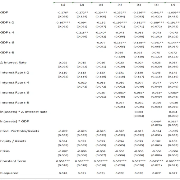
26 Due to the change of significance of the GDP’s, variations of lagged GDP with longer
cycles were tested. Thus, lags of two quarters of GDP and Interest Rate were assessed, and the other control variables were kept, as presented in Table 6.
Table 6 – Provision to Non-Performing Loans (NPL) on Two-Quarter Lags of GDP and of Interest Rates, as well as other banking system characteristics
Table 6 presents panel result with estimation per fixed effects, considering the correction for heteroscedasticity. GDP stands for quarterly economic growth rate, GDP t-n is the GDP growth rate verified in “n” previous quarters. Delta Interest rate means the variation of interest rate equivalent to the verified year throughout the period. Interest rate t-x corresponds to the Selic interest
rate verified in the “n” previous quarter. Credit Portfolio/Assets is the bank’s loan level, given by the relation between the credit
portfolio and its total assets. Equity/ Assets is the financing level of assets per own capital, given by the relation between Equity and Assets of each financial institution. Ln(assests)* Delta Interest Rate is the natural log of assets of each financial institution multiplied by interest rate variation. Ln(assets)*GDP is the natural log of assets of each financial institution multiplied by the quarterly economic growth rate. Crisis is the is a Dummy Control variable, which corresponds to the periods from October, 2001, to December, 2002, and October, 2008, to December, 2009. *, ** and *** indicate significance of 10%, 5%, and 1%, respectively.
27
In the first specification (Table 6, column 1),
𝑁𝑃𝐿𝑖, =
𝛽0𝑖, + 𝛽1𝐺 𝑃𝑖, +𝛽2𝐺 𝑃𝑖, −2 +𝛽3𝛥𝐼 .𝑅𝑎 𝑖, +𝛽4𝑅 𝑎 𝐼 .𝑅𝑎 𝑖, −2 + 𝛽5 𝑖𝐴𝑃 𝑖 𝑖, +𝛽6𝐴 𝑖 𝑦 𝑖, +𝛽7 𝑖, +ℯ (1) ,
GDP and GDP t-2 behaved according to our expectation with significance levels well below 10% and 1%, respectively and their betas were higher -0.176 and -0.167, respectively. Therefore, this result supports the theory that the performance loan portfolios of Brazilian commercial banks improves when the GDP increases. However, the interest rate variables remained insignificant.
In the second specification (Table 6, column 2), GDP and GDP t-4 presented significance levels below 5% and their betas, -0.272 and -0.215 respectively, were higher than the previous specifications.
In the third specification (Table 6, column 3), the GDP presented significance levels at 5%, and GDP t-4 at 10%, but their betas were lower than the previous specification. The interest rate variables remained insignificant.
In the fourth specification (Table 6, column 4), GDP and GDP t-6 presented significance levels at 5% and GDP t-2 at 1% with betas of -0.232, -0.153 and -0.199 respectively. Thus, it is noticed that NPL responds better to GDP variation with two- quarter lags.
From the fifth through the seventh specification, control variables “natural log of assets” of each financial institution multiplied by Interest Rate (ln(assets) x interest rate variation) and “natural log of assets” multiplied by quarterly economic growth (ln(assets)*GDP) were added because the assets size of banks can significantly affect the loan portfolio performance of the banks.
28 𝑁𝑃𝐿𝑖, = 𝛽0𝑖, + 𝛽1𝐺 𝑃𝑖, +𝛽2𝐺 𝑃𝑖, −2 +𝛽3𝐺 𝑃𝑖, −4 +𝛽4𝐺 𝑃𝑖, −6 + 𝛽5𝐺 𝑃𝑖, −8 +𝛽6𝛥𝐼 .𝑅𝑎 𝑖, +𝛽7𝑅 𝑎 𝐼 .𝑅𝑎 𝑖, −2 +𝛽8𝑅 𝑎 𝐼 .𝑅𝑎 𝑖, − 4 +𝛽9𝑅 𝑎 𝐼 .𝑅𝑎 𝑖, −6 +𝛽10𝑅 𝑎 𝐼 .𝑅𝑎 𝑖, −8 +
𝛽11 ln assets x𝛥𝐼 .𝑅𝑎 𝑖, +𝛽12 𝑖 𝑃 𝑖
𝐴 𝑖, +𝛽13 𝑖 𝑦
𝐴 𝑖, +𝛽14 𝑖, + ℯ (5)
it is shown that the addition of variable “ln(assets)*interest rate variation” (table 6, column 5) was not statistically significant, and the explanatory variables for GDP and interest rate kept the statistical significant levels of the previous specifications.
In the sixth specification (Table 6, column 6), the variable “ln(assets)xGDP” was added.
𝑁𝑃𝐿𝑖, = 𝛽0𝑖, + 𝛽1𝐺 𝑃𝑖, +𝛽2𝐺 𝑃𝑖, −2 +𝛽3𝐺 𝑃𝑖, −4 +𝛽4𝐺 𝑃𝑖, −6 + 𝛽5𝐺 𝑃𝑖, −8 +𝛽6𝛥𝐼 .𝑅𝑎 𝑖, +𝛽7𝑅 𝑎 𝐼 .𝑅𝑎 𝑖, −2 +𝛽8𝑅 𝑎 𝐼 .𝑅𝑎 𝑖, − 4 +𝛽9𝑅 𝑎 𝐼 .𝑅𝑎 𝑖, −6 +𝛽10𝑅 𝑎 𝐼 .𝑅𝑎 𝑖, −8 +𝛽11ln(assets)x𝐺 𝑃𝑖, +
𝛽12 𝑖 𝑃 𝑖
𝐴 𝑖, +𝛽13 𝑖 𝑦
𝐴 𝑖, +𝛽14 𝑖, +ℯ (5)
As a result of this new specification, the variable "ln(assets) x GDP" was statistically significant at 10% with positive sign, which shows that the size of assets affects
negatively the performance of Brazilian commercial banks’ loan portfolio. Moreover,
we can conclude that the GDP changes have more influence on banks with greater assets.
In the seventh specification (Table 6, column 7), both variables “ln(assets) x Interest
Rate Variation” and GDP” “ln(assets)xGDP” were added. The results were similar to
the ones previously obtained, only “ln(assets)xGDP” showed statistical significant at
10% level.
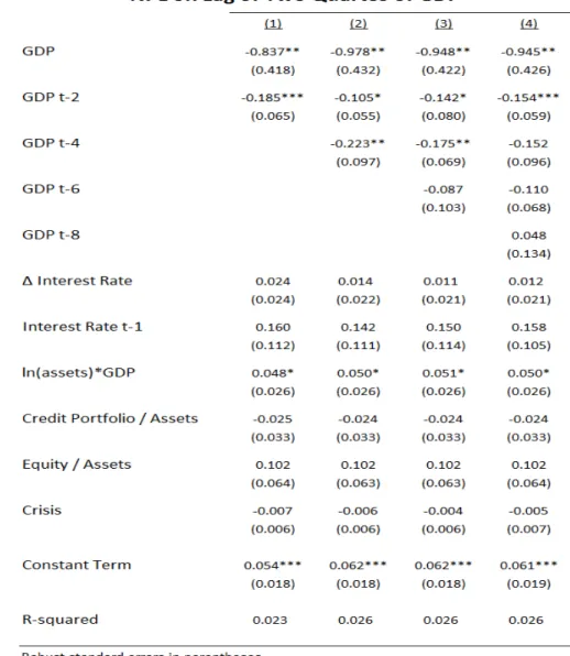
29 Glen and Velez's model, and the variable “ln(assets)xGDP” was kept because its
statistical significance level. The results are presented in Table 7.
Table 7 – Provision to Non-Performing Loans (NPL) Regressions on Two-Quarter
Lags of GDP and Interest Rate
Table 7 presents panel result with estimation per fixed effects, considering the correction for heteroscedasticity GDP stands for quarterly economic growth rate, GDP t-n is the GDP growth rate verified in “n” previous quarters. Interest rate Var. means the variation of interest rate equivalent to the verified year throughout the period. Interest rate t-1 corresponds to the Selic interest rate verified in the previous quarter. Ln(assets)*GDP is the natural log of assets of each financial institution multiplied by the quarterly economic growth rate. Credit Portfolio/Assets is the bank’s loan level, given by the relation between the credit portfolio
and its total assets. Equity/ Assets is the financing level of assets per own capital, given by the relation between Equity and Assets of each financial institution. Crisis is a Dummy Control variable, which corresponds to the periods from October, 2001, to December, 2002 e Out, 2002, and October, 2008 a Dez.2008, to December, 2009. *, ** and *** indicate significance of 10%, 5%, and 1%, respectively.
30
In the first specification (Table 7, column 1),
𝑁𝑃𝐿𝑖, =
𝛽0𝑖, + 𝛽1𝐺 𝑃𝑖, +𝛽2𝐺 𝑃𝑖, −2 +𝛽3𝛥𝐼 .𝑅𝑎 𝑖, +𝛽4𝑅 𝑎 𝐼 .𝑅𝑎 𝑖, −1 + 𝛽5 ln assets x𝐺 𝑃𝑖, +𝛽6 𝑖𝐴𝑃 𝑖 𝑖, +𝛽7𝐴 𝑖 𝑦 𝑖, +𝛽8 𝑖, +ℯ (1),
GDP and GDP t-2 presented the expected signs and significant at 1%, reinforcing the fact that GDP variations explain more significantly the variations of the level of performance of Brazilian commercial banks, with a two-quarter lag, and that the interest rate variation has no statistical significance to explain the level of
performance of banks’ credit portfolio. Besides, the GDP and GDP t-2 betas were high, -0.170 and 0.178, respectively. The ln(assets)*GDP variable presented the expected signs and significant at 10%.
In the second specification (Table 7, column 2), with the addition of the GDP t-4 variable, GDP and GDP t-4 were significant at 5%, and GDP t-2, at 10%.
In the third specification (Table 7, column 3), with the addition of the GDP t-6 variable, GDP, GDP t-2 and GDP t-4 kept the significant levels of the previous specification, but their betas were worse. The GPD t-6 did not present statistical significance.
In the fourth specification (Table 7, column 4), with the addition of the GDP t-8 variable, only GDP and GDP t-2 were significant at 5% and 1%, respectively.
Thus, it is noticed that NPL (provision for non-performing loan) responds better to GDP variations with two-quarter lags, considering a 1-year timeframe.
31 𝑁𝑃𝐿𝑖, = 𝛽0𝑖, + 𝛽1𝐺 𝑃𝑖, +𝛽2𝐺 𝑃𝑖, −2 +𝛽3𝐺 𝑃𝑖, −4 +𝛽4𝛥𝐼 .𝑅𝑎 𝑖,
+𝛽5𝑅 𝑎 𝐼 .𝑅𝑎 𝑖, −1 +𝛽6 ln assets x𝐺 𝑃𝑖,
+𝛽7 𝑖 𝑃 𝑖
𝐴 𝑖, +𝛽8
𝑖 𝑦
𝐴 𝑖, +𝛽9 𝑖, +ℯ (2)
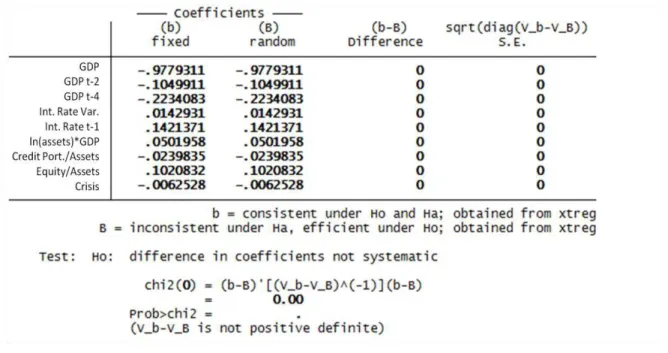
The results are described in the table below:
Table 8 – Testing for Endogeneity (Hausman Test)
Table 8 presents the results of the Hausman Test, which evaluates the significance of an estimator versus an alternative estimator. GDP stands for quarterly economic growth rate, GDP t-n is the GDP growth rate verified in “n” previous quarters.
Interest rate Var. means the variation of interest rate equivalent to the verified year throughout the period. Interest rate t-1 corresponds to the Selic interest rate verified in the previous quarter. Ln(assets)*GDP is the natural log of assets of each financial institution multiplied by the quarterly economic growth rate. Credit Portfolio/Assets is the bank’s loan level, given by the
relation between the credit portfolio and its total assets. Equity/ Assets is the financing level of assets per own capital, given by the relation between Equity and Assets of each financial institution. Crisis is a Dummy Control variable, which corresponds to the periods from October, 2001, to December, 2002, and October, 2008, to December, 2009.
Source: own elaboration
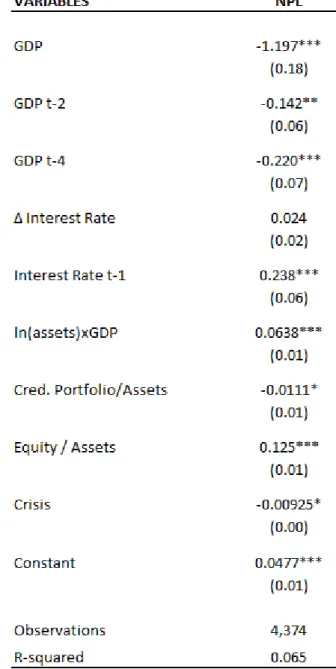
32
Table 9 – Results of 2SLS regression
Table 9 presents the results of the second stage of two-stage regression (2SLS Regression) with robust standard errors. GDP stands for quarterly economic growth rate, GDP t-n is the GDP growth rate verified in “n” previous quarters. Interest rate Var. means the variation of interest rate equivalent to the verified year throughout the period. Interest rate t-1 corresponds to the Selic interest rate verified in the previous quarter. Ln(assets)*GDP is the natural log of assets of each financial institution multiplied by the quarterly economic growth rate. Credit Portfolio/Assets is the bank’s loan level, given by the relation between
the credit portfolio and its total assets. Equity/ Assets is the financing level of assets per own capital, given by the relation between Equity and Assets of each financial institution. Crisis is a Dummy Control variable, which corresponds to the periods from October, 2001, to December, 2002, and October, 2008, to December, 2009. *, ** and *** indicate significance of 10%, 5%, and 1%, respectively.
33
34 4.1 Robustness Check
To test the robustness of the significance of NPL, the measures of GPD and Interest Rates was replaced by GPD and Interest Rates with different lags. The results are described in the table below:
Table 10 – Robustness Check
Table 10 presents the results of the second stage of two-stage pooled regression (2SLS Regression) with robust standard errors. GDP stands for quarterly economic growth, GDP t-n is the GDP growth verified in “n” previous quarters. Interest rate Var. means the variation of interest rate equivalent to the verified year throughout the period. Interest rate t-1 corresponds to the Selic interest rate verified in the previous quarter. Ln(assets)*GDP is the natural log of assets of each financial institution multiplied by the quarterly economic growth rate. Credit Portfolio/Assets is the bank’s loan level, given by the relation between
the credit portfolio and its total assets. Equity/ Assets is the financing level of assets per own capital, given by the relation between Equity and Assets of each financial institution. Crisis is a Dummy Control variable, which corresponds to the periods from October, 2001, to December, 2002, and October, 2008, to December, 2009. *, ** and *** indicate significance of 10%, 5%, and 1%, respectively.
35
36
5. CONCLUSION
This paper tested the effects of economic growth (GDP), as well as the interest rate upon the performance of loan portfolios of Brazilian commercial banks from 2000 through 2010, taking into account the assessment model used by Glen and Velez (2010).
The empirical result showed that the economic growth (GDP) is the main driver of the performance of the credit portfolio of Brazilian commercial banks, and that the variation in the interest rate has no significant effects on it. Such fact could be explained by the practice of renegotiation, debts lengthening, and by the adoption of a conservative credit policy conducted by Brazilian banks, which occur more frequently during periods of crisis.
Furthermore, the results showed that the GDP variations correlated significantly with the performance level variations of Brazilian commercial banks, with a two-quarter lag throughout the period of one year.
Finally, the results showed that changes in GDP most significantly impact on the
performance of the largest Brazilian commercial banks’ loan portfolio. Due to the
37 6. REFERENCE
AKERLOF, G. A. (1970). The market for “lemons”: qualitative uncertainty and the market
mechanism. Quartely Journal of Economics. Cambridge, v. 84, n. 3, p. 488-500.
ALTMAN, E. L. (1968). Financial ratios, discriminant analysis, and the prediction of corporate Insolventecy. Journal of Finance, p. 589-609.
ANDRADE, F. W. M. (2003). Modelos de Risco de Crédito. Tecnologia de Crédito, n. 38, p.
23-53.
ARRAES, R. A. & TELLES, V. K. (2000). Endogeneidade e exogeneidade do crescimento econômico: uma análise comparativa entre Nordeste, Brasil e países selecionados. Revista Econômica do Nordeste, 31. p. 754-776, Fortaleza, Brazil.
BACEN (2011). 50 maiores bancos e o consolidado do sistema financeiro nacional
<http://www.bcb.gov.br>.
BACEN (2011). Taxa Selic. <http://www.bcb.gov.br>.
BASEL COMMITTEE ON BANKING SUPERVISION (1998). International convergence of capital measurement and capital standards. Bank for International Settlements.
BASEL COMMITTEE ON BANKING SUPERVISION (2004). International convergence of capital measurement and capital standards: a revised framework. Bank for International Settlement.
BERGER, A. N.; DEYOUNG, R. (1997). Problem loans and cost efficiency in commercial banks. Journal of Banking and Finance,v. 21, p. 849-870.
BERGER, A. N.; HANNAN, T. H. (1989).The price-concentration relationship in banking. Review of Economics and Statistics, v. 71, p. 291-299.
BERNANKE, B.; GERTLER, M.; GILCHRIST, S. (1998). The financial accelerator in a quantitative business cycle framework, Working Paper 6455, Cambridge: NBER, p.75.
BERNANKE, B. (1983). Non-monetary effects of the financial crisis in the propagation of the Great Depression. American Economic Review. Nashville, v. 73, n. 3, p. 257-276.
BESSIS, Joel. (1998). Risk management in banking. Chichester: John Wiley & Sons.
BONELLI, R. (1991). Crescimento e produtividade na indústria brasileira: impactos da orientação comercial. Pesquisa e Planejamento Econômico, 21(3), pp.533-58.
CAOUETTE, John B. Et al. (2000). Gestão do Risco de Crédito: o próximo grande desafio financeiros. Qualitymark, Rio de Janeiro.
38
CHANG, E.; GUERRA, S.; LIMA, E.; TABAK, B. (2008).The stability–concentration relationship in the Brazilian banking system. Int. Fin. Markets, Inst. and Money, 18, p. 388–
397.
CHU, V. (2001). Principais fatores macroeconômicos da inadimplência bancária no brasil. In: BANCO CENTRAL DO BRASIL. Juros e spread bancário no Brasil: avaliação de dois anos do projeto, p. 41-45,
CIRCULAR 3.398 (2008). Estabelece procedimentos para a remessa de informações relativas à apuração dos limites e padrões mínimos regulamentares que especifica. Banco Central do Brasil.
FAVA, V. L.; CATI, R. C. (1995). Mudanças no comportamento do PIB brasileiro: uma abordagem econométrica. Pesquisa e Planejamento Econômico, Rio de Janeiro, v. 25, n. 2,
p. 279-296.
FERREIRA, P. C. (1996). Investimento em infra-estrutura no Brasil: fatos estilizados e relações de longo prazo. Pesquisa e Planejamento Econômico, 26(2), p.231-52.
MALLIAGROS, T. G. (1998). Impactos produtivos da infra-estrutura no Brasil – 1950/95. Pesquisa e Planejamento Econômico, 28(2), p.315-37.
FERREIRA, P. C.; ISSLER, J. V. (1997). Educação e Crescimento. In: FONTES, R. Estabilização e Crescimento. cap. 14, p. 297-313.
FILIPPAKI, A. K.; MAMATZAKIS, E. (2009). Performance and Merton-Type Default Risk of Listed Banks in EU: a panel VAR approach, Discussion Paper Series 2009_09, Department of Economics, University of Macedonia.
FISHER, I. (1933). The debt-deflation theory of great depressions. Econometrica. Chicago, v. 1, n. 4, p. 337-357.
FRIEDMAN, M.; SCHWARTZ, A. (1963). A monetary history of the United States: 1867-1960. Princeton: Princeton University Press, p.888.
GAMBACORTA, L. (2008). How do banks set interest rates? European Economic Review, v. 52, p. 792-819.
GARCIA, M. G. P. (1996). O financiamento à infra-estrutura e a retomada do crescimento econômico sustentado. Revista de Economia Política, v. 16, p. 5-19.
GERTLER, M. (1988). Financial structure and aggregate economic activity: an overview. Cambridge: (Working Paper, 2559,) p.53.
GLEN, J.; VÉLEZ, C. M. (2010). Business Cycle Effects on Commercial Bank Loan Portfolio Performance in Developing Economies. International Finance Corporation.
39
GONZAGA, G.; ISSLER, J. V.; MARONE, G. (1995). Educação, investimentos externos e crescimento econômico: evidências empíricas. Rio de Janeiro: PUC.
HO, T.; SAUNDERS A. (1981). The determinants of bank interest margins: Theory and empirical evidence. Journal of Financial and Quantitative Analysis, p. 581-600.
HOUAISS A. (2001). Dicionário Houaiss da Língua Portuguesa. Rio de Janeiro
IBGE (2011). PIB a preços de mercado. Sistema de Contas Nacionais, 2010a.
<http://www.ipeadata.gov.br/>.
INTERNATIONAL MONETARY FUND (2010). Global Financial Stability Report. IMF, Washington D.C.
JORION, Philippe. (2003). Value at Risk: a nova fonte de referência para a gestão do risco financeiro. 2º ed. BM&F. São Paulo.
KASHYAP, A.; STEIN, J. (2000). What do a million observations on banks say about the transmission of monetary policy. American Economic Review, 90, p. 407-428.
KEYNES, J. M. (1936). The General Theory of Employment, Interest and Money. London: Macmillan Press.
KOYAMA, S. M.; NAKANE, M. I. (2002) “Os Determinantes do Spread Bancário no Brasil”,
Banco Central do Brasil, Nota Técnica n. 17.
LLEDÓ, V. D.; FERREIRA, P. C. (1997) Crescimento endógeno, distribuição de renda e política fiscal: uma análise cross-section para os estados brasileiros. Pesquisa e Planejamento Econômico, 27(1), p.41-69.
LOUZIS D. P., VOULDIS A. T., METAXAS V. L. (2010). Macroeconomic and Bank specific Determinants of Nonperforming Loans in Greece: A Comparative Study of Mortgage, Business, and Consumer Loan Portfolios. Bank of Greece, Working Paper 118.
MISHKIN, F. S. (1978). The household balance sheet and the Great Depression. Journal of Economic History, New York, v. 38, n. 4, p. 918-37.
NEVES, S.; VICECONTI, P. E. V. (1998). Contabilidade Avançada. São Paulo
PAIN, D. (2003).The provisioning experience of the major UK banks: a small panel investigation. London: Bank of England, p.41.
PARENTE, G. G. C. (2000). As novas normas de classificação de crédito e o disclosure das provisões. Uma abordagem introdutória. In: 9ª. Semana de Contabilidade do Banco Central do Brasil.