A Survey on Fault Localization Techniques

A Survey on Fault Localization Techniques

Alexandre Perez, Rui Abreu Department of Informatics Engineering Faculty of Engineering, University of Porto

Porto, Portugal

alexandre.perez@fe.up.pt, rui@computer.org

W. Eric Wong

Department of Computer Science University of Texas at Dallas

Richardson, Texas, USA ewong@utdallas.edu

Abstract—A considerable body of work on debugging and particularly in fault localization has been published in the past decades. This paper summarizes the underlying ideas behind locating faults and presents the different techniques that are currently available to tackle the challenging task that is diagnosing faulty software systems and groups them into different categories: traditional debugging techniques (such as assertions and breakpoints), program slicing, delta debugging and coverage-based, as well as model-based approaches to debugging are detailed. A comparison between such diagnosis techniques is performed, and the challenges and potential fu-ture directions of software fault localization are also discussed.

Keywords-Debugging, diagnosis, fault localization, software testing.

I. INTRODUCTION

In 1947, the Harvard Mark II was being tested by Grace Murray Hopper and her associates when the machine sud-denly stopped. Upon inspection, the error was traced to a dead moth that was trapped in a relay and had shorted out some of the circuits. The insect was removed and taped to the machine’s logbook [1]. This incident is believed to have coined the use of the terms “bug”, “debug” and “debugging” in the field of computer science. Since then, the term debugging is associated to the process of detecting, locating and fixing faulty statements in computer programs. In software development, a large amount of resources is spent in the debugging phase. It is estimated that testing and debugging activities can easily range from 50 to 75 percent of the total development cost [2]. This is due to the fact that the process of detecting, locating and fixing faults in the source code is not trivial and is error-prone. Even experienced developers are wrong almost 90% of the time in their initial guess while trying to identify the cause of a behavior that deviates from the intended one [3].

If this debugging task is not thoroughly conducted, even bigger costs may arise. In fact, a landmark study performed in 2002 indicated that software defects constitute an annual $60 billion cost to the US economy alone [4].

Debugging, as well as testing, are then important steps that should not be disregarded when developing software. However these tasks consume large amounts of resources. Therefore, ways to help developers in these tasks are

continuously being researched. Currently, there are some techniques that (semi)automatically pinpoint likely sources of faults in software programs. Different from a previous survey [5], this paper groups fault localization techniques from an alternative perspective and discusses and compares them.

This paper makes the following contributions:

• Several software fault localization techniques and tools currently in use are detailed, namely traditional debug-ging, program slicing, delta debugdebug-ging, coverage-based and model-based approaches.

• A comparison between such fault localization tech-niques is performed.

The remainder of this paper is structured as follows. Section II will introduce some concepts used throughout the paper. Section III will present some traditional debugging techniques (e.g., assertions and breakpoints). In Section IV, program slicing will be detailed. Section V will present delta debugging. Coverage-based debugging approaches are detailed in Section VI, and reasoning-based approaches appear in Section VII. Section VIII will provide a compar-ison between the previously detailed debugging techniques. Lastly, some conclusions are drawn in Section IX.

II. CONCEPTS& DEFINITIONS

In this section, some concepts and definitions are intro-duced. Throughout this paper, the following terminology is used [6]:

• A failure is an event that occurs when delivered service deviates from correct service.

• An error is a system state that may cause a failure. • A fault (defect/bug) is the cause of an error in the

system.

In this paper, this terminology is applied to software pro-grams, where faults are bugs in the program code. Failures and errors are symptoms caused by faults in the program. The purpose of fault localization is to pinpoint the root cause of observed symptoms.

Definitions of software programs, test suites and test cases used throughout this paper should also be mentioned:

Definition 1 A software program Π is formed by a sequence M of one or more statements.

Definition 2 A test suite T = {t1, . . . , tN} is a collection

of test cases that are intended to test whether the program follows the specified set of requirements. The cardinality of T is the number of test cases in the set |T | = N .

Definition 3 A test case t is a (i, o) tuple, where i is a collection of input settings or variables for determining whether a software system works as expected or not, and o is the expected output. If Π(i) = o the test case passes, otherwise fails.

III. TRADITIONALDEBUGGING

In this section, traditional debugging techniques and tools are described, namely print statements, assertions, break-points, profiling and code coverage.

A. Print Statements

A common, ad-hoc approach to locate bugs when a program shows some abnormal behavior is to insert print statements to print extra information to help debug the misbehavior. Each of these statements causes the program to output the value of a certain variable. This way, additional information about both the runtime state and control flow can be shown to help developers identify the root cause of the failure.

B. Assertions

Assertions are formal constraints that the developer may use to specify what the system is supposed to do (rather than how) [7]. These constructs are generally predefined macros that expand into an if statement that aborts the execution if the expression inside the assertion evaluates to false. Assertions can be seen, then, as permanent defense mechanisms for runtime fault detection.

C. Breakpoints

A breakpoint specifies that the control of a program execution should transfer to the user when a specified instruction is reached [8]. The execution is stopped and the user can inspect and manipulate the program state (e.g., the user can read and change variable values). It is also possible to perform a step-by-step execution after the breakpoint. This is particularly useful to observe a bug as it develops, and to trace it to its origin.

There are other types of breakpoints, namely data break-points and conditional breakbreak-points. Data breakbreak-points (also called watchpoints [9]) transfer control to the user when the value of an expression changes. This expression may be a value of a variable, or multiple variables combined by operators (e.g., a + b). Conditional breakpoints only stop the execution if a certain user-specified predicate is true, thus reducing the frequency of user-application interaction.

D. Profiling

Profiling is a dynamic analysis that gathers some metrics from the execution of a program, such as memory usage and frequency and duration of function calls. Profiling’s main use is to aid program optimization, but it is also useful for debugging purposes, such as:

• Knowing if functions are being called more or less often

than expected;

• Finding if certain portions of code execute slower than

expected or if they contain memory leaks;

• Investigating the behavior of lazy evaluation strategies. Known profiling tools include GNU’s gprof1 _{and the}

Eclipse plugin TPTP2. E. Code Coverage

Code coverage is an analysis method that determines which parts of the System Under Test (SUT) have been executed (covered) during a system test run [10].

Using code coverage in conjunction with tests, it is possible to see which lines of code, methods or classes were covered in a specific test (depending on the set level of detail). With this information, it is possible to identify which components were involved in a system failure, narrowing the search for the faulty component that made the test fail.

Pre Relocated Instruction Post Program Base Trampoline Save Registers Set up Args Snippet Restore Registers foo() Mini Trampoline

Figure 1: Instrumentation Code Insertion [11].

In order to obtain information about what components were covered in each run, these code coverage tools have to instrument the system code. This instrumentation will monitor each component and register if they were executed. Instrumentation code, as depicted in Figure 1, relies on a series of trampolines to a function foo() before the desired instructions. In the case of Cove Coverage tools, foo() will register that the instruction was touched by the execution.

IV. PROGRAMSLICING

In 1981, Weiser introduced static program slicing [12], [13]. This technique starts from the failure and uses the

1_{GNU gprof – http://sourceware.org/binutils/docs/gprof/}

2_{Eclipse Test & Performance Tools Platform Project – http://www.} eclipse.org/tptp/

control and data flow of the program as a backwards reason-ing method to reach the fault location. It narrows down the covered statements of a software program by removing all statements that have no data or control dependencies to these variables of interest responsible for detecting the failure. A slice can be seen as a subset of program statements that directly or indirectly influence the values of a given set of variables of interest. Debugging consists of inspecting the statements that comprise the slice, rather than looking at the entire program.

A slice that is computed only by means of static analysis tends to be large. Lyle and Weiser were able to reduce the number of statements that need to be examined by constructing a program dice [14]. Program dice is the set difference between static slices of incorrect and correct variables. However, there are some statements that can only be excluded by predicting run-time values. For this reason, dynamic program slicing was introduced by Korel et al. [15]. Dynamic program slicing relies on execution information to determine what statements belong to the slice (or dice), and can significantly reduce the size of the slice.

Dynamic slices occasionally omit statements that were responsible for the fault. This can happen when the faults cause certain parts of the program to stop being executed. To eliminate this problem, Zhang et al. introduced the concepts of implicit dependencies and relevant slicing [16], [17], where dependencies can also be obtained by predicate switching.

Another dynamic approach to program slicing was pro-posed by Wong et al., using execution slices [18] and inter-block data dependencies [19]. This approach uses sets of code (such as basic blocks) as the building blocks for a slice. Two blocks are data dependent if one block contains a definition that is used by another block or vice versa. This approach will include additional code for inspection but is less likely to omit potentially interesting statements.

V. DELTADEBUGGING

Delta debugging is a technique that tries to systemati-cally simplify the input that leads a certain program to a failure [20]. The idea is to iteratively reduce the size of the input until the smallest input that causes the execution to fail is reached [21], [22]. This is done under the assumption that that smaller inputs cover less lines of code than larger inputs and thus are easier to debug. It is also assumed that inputs can be stripped down and simplified, which may not always be true.

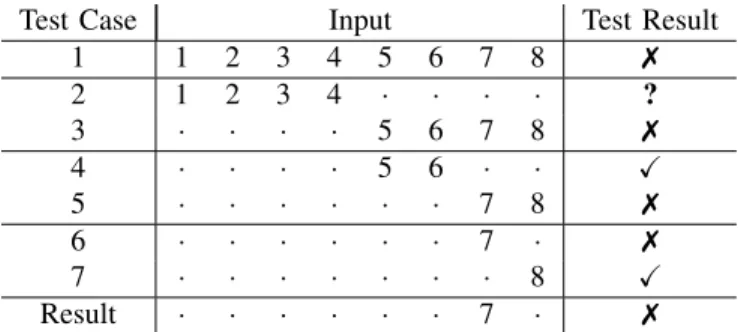
Figure 2 depicts the delta debugging technique. Suppose a program takes as input a set of integers ranging from 1 to 8. In order to use delta debugging, an initial input is devised, which encompasses all possible elements in the set (test case 1 in the figure). As this test case fails, the next step is to remove inputs from the next test cases, as is the case in test case 2 and 3. One thing to note is that by manipulating

Test Case Input Test Result

1 1 2 3 4 5 6 7 8 ₇ 2 1 2 3 4 · · · · ? 3 · · · · 5 6 7 8 ₇ 4 · · · · 5 6 · · _X 5 · · · 7 8 7 6 · · · 7 · ₇ 7 · · · 8 _X Result · · · 7 · 7

Figure 2: Delta debugging example (adapted from [20]).

input, one can reach a third test case outcome besides passed (_{X) and failed (7). This outcome is called unresolved (?)} and normally happens when invalid input is passed to the program. The next steps of the delta debugging algorithm are to keep dividing the input size for test cases that lead to failures (_{7). In this example, test 3 is expanded into tests 4} and 5. After that, test 5 is expanded into tests 6 and 7. As can be seen in the figure, test 6 produces the minimal input for which there is still a failure, so the result of the technique is the set of cardinality 1, encompassing the element 7.

A practical example of the use of delta debugging is when debugging graphical user interfaces (GUIs). Suppose that you have a sequence of GUI operations that cause an application to crash. Assuming that the crash can be replayed automatically, delta debugging can be used to iteratively remove GUI operations until a minimum collection of op-erations that still cause the program to crash is reached. This new sequence, as it contains the same error as the original one, but contains less operations, will cover less code, helping developers narrow down the code locations they need to inspect.

Delta debugging considers the input as a flat atomic list. This list is usually large and may contain a vast amount of information irrelevant to the failure. In order to avoid many spurious input combinations, Misherghi et al. have proposed the Hierarchical Delta Debugging technique [23]. This technique takes into account the input structure so that fewer input configurations need to be attempted. Initially using a coarser level of detail, the algorithm is able to prune large irrelevant portions of the input early. Besides speeding up the Delta Debugging process, this hierarchical technique also has the advantage of producing better (and more easily understandable) diagnostic reports, as the output is a structured tree.

VI. COVERAGE-BASEDAPPROACHES

In this section, coverage-based approaches to debugging are presented. First, the concept of program spectra is in-troduced. Afterwards, the spectrum-based fault localization and the dynamic code coverage techniques are detailed.

A. Program Spectra

A program spectrum is a characterization of a program’s execution on an input collection [24]. This collection of data consists of counters of flags for each software component, and is gathered at runtime. Software components can be at several detail granularities, such as classes, methods or lines of code. A program spectrum provides a view on the dynamic behavior of the system under test [25].

Recording program spectra is a lightweight analysis method. In order to obtain information about which compo-nents were covered in each execution, the program’s source code needs to be instrumented, similarly to what happens in code coverage tools (see Section III-E). This instrumentation will monitor each component and register those that were executed.

B. Spectrum-based Fault Localization

Spectrum-based Fault Localization (SFL) is a statistical debugging technique that, for each software component, calculates the likelihood of it being faulty [26]. It exploits information from passed and failed system runs. A passed run is a program execution that is completed correctly, and a failed run is an execution where an error was detected [27]. The criteria for determining if a run has passed or failed can be from a variety of different sources, namely test case results and program assertions, among others. The execution information gathered for each run is their program spectra. As SFL focuses only on registering whether a component is touched or not during a certain execution, so binary flags can be used for each component. This particular form of program spectra is also called hit spectra [25].

The hit spectra used by SFL is a binary N × M matrix A, where N corresponds to the number of passed/failed runs and M corresponds to the instrumented components of the program. Information of passed and failed runs is gathered in an N -length vector e, called the error vector. The pair (A, e) serves as input for the SFL technique.

With this input, the next step in this coverage-based technique consists of determining what columns of the matrix A resemble the error vector e the most. This is done by calculating the resemblance between these two vectors by means of similarity coefficients [28].

Several similarity coefficients do exist [27]. Examples of similarity coefficients are shown below, namely the Jaccard coefficient sJ used in the Pinpoint tool [29], the sA

coeffi-cient used by the AMPLE [30] tool and the sT coefficient

used in the Tarantula3 _{tool [26], [31]:}

sJ(j) = n11(j) n11(j) + n01(j) + n10(j) (1) sA(j) =     n11 n01+ n11 − n10 n00+ n10     (2) 3_{Available at http://pleuma.cc.gatech.edu/aristotle/Tools/tarantula/} sT(j) = n11(j) n11(j)+n01(j) n11(j) n11(j)+n01(j)+ n10(j) n10(j)+n00(j) (3) where npq(j) is the number of runs in which the component

j has been touched during execution (p = 1) or not touched during execution (p = 0), and where the runs failed (q = 1) or passed (q = 0). For instance, n11(j) counts the number of

times component j has been involved in failed executions, whereas n10(j) counts the number of times component j

has been involved in passed executions. Formally, npq(j) is

defined as:

npq(j) = |{i | aij = p ∧ ei= q}| (4)

One of the best performing similarity coefficients for fault localization is the Ochiai coefficient [32]. The fault local-ization tools Zoltar [33] and GZoltar4 [34] use the Ochiai coefficient to quantify the resemblance to the error vector. This coefficient was initially used in the molecular biology domain [35], and is defined as follows:

sO(j) =

n11(j)

p(n11(j) + n01(j)) · (n11(j) + n10(j))

(5) The similarity coefficients that were calculated can rank the software components according to their likelihood of containing the fault. This is done under the assumption that a component with a high similarity to the error vector has a higher probability of being the cause of the observed failure than a component with low similarity. A list of the software components, sorted by their similarity coefficient, is then presented to the developer. This list is also called diagnostic report, and helps developers prioritize their inspection of software components to pinpoint the root cause of the observed failure.

One problem with Tarantula and many similarity coefficient-based fault localization techniques such as those discussed above is that they do not distinguish the contribu-tion of one failed test case from another, or one successful test case from another. To overcome this problem, Wong et al. [36] proposed that, with respect to a piece of code, the contribution of the nth failed test in computing its suspiciousness is larger than or equal to that of the (n + 1)th failed test. The same applies to the contribution provided by successful tests. In addition, the total contribution of the failed tests is larger than that of the successful. Techniques discussed in [36] are named as H3b and H3c.

Using the same set of information as other spectrum-based fault localization techniques, Wong et al. presented a crosstab analysis-based approach [37], where a crosstab is constructed for each statement with two column-wise categorical variables “covered” and “not covered”, and two row-wise categorical variables “successful execution” and “failed execution.” A hypothesis test is used to provide a

reference of “dependency/independency” between the exe-cution results and the coverage of each statement. However, the exact likelihood of each statement depends on the degree of association (instead of the result of the hypothesis testing) between its coverage (number of tests that cover it) and the execution results (success/failure).

Wong et al. also proposed two fault localization tech-niques using program spectra data based on a back-propagation (BP) neural network [38] and a modified radial basis function (RBF) neural network [39], respectively. The coverage data of each test case and the corresponding execution result are used to train a neural network so that it can learn the relationship between them. Then, the coverage of a set of virtual test cases that each covers only one statement in the program are input to the trained network, and the outputs can be regarded as the likelihood of each statement containing the bug.

A technique named DStar (D∗) is reported by Wong et al. [40] such that the likelihood of a statement j being faulty is (1) proportional to the number of failed tests that cover it (n11(j)), (2) inversely proportional to the number

of successful tests that cover it (n10(j)), and (3) inversely

proportional to the number of failed tests that do not cover it (n01(j)). More importantly, (1) is the most sound intuition

and should carry a higher weight than (2) and (3). That is, we should assign greater importance to the information obtained from observing which statements are covered by failed tests than that obtained from observing which statements are covered by successful tests or which are not covered by failed tests. Together, for a statement j, its likelihood of containing program bugs is computed as n11(j)∗

(n01(j)+n10(j))

where ∗ ≥ 1. The effectiveness of D∗ increases as ∗ grows, and then levels off when ∗ exceeds a critical value.

Empirical data suggests that D∗ is in general more effec-tive at locating bugs than the RBF-technique (which outper-forms H3b, H3c, Ochiai, and the Crosstab-based technique). Furthermore, they are all better than Tarantula and many similarity coefficient-based techniques.

To solve the test oracle issue, Xie et al. developed an SFL technique based on metamorphic slice for program debugging without a test oracle [41]. Test cases are replaced by corresponding metamorphic test groups, and execution results of failure or success are indicated by whether some metamorphic relations are violated. Another solution was proposed by Abreu et al., using low cost, generic invariants (“screeners”) as error detectors for fault localization [42].

Coverage-based techniques have shown good evaluation results for a single fault, but their ability to diagnose multiple faults is limited. To address this, Steimann et al. proposed a technique that uses integer linear programming to partition coverage matrices [43]. This partitioning breaks down the fault localization problem into several smaller ones, which can be dealt independently.

SFL can be used with program spectra of several different

granularities. However, it is most commonly used at the line of code level. Using coarser granularities would be difficult for programmers to investigate if a given fault hypothesis generated by SFL was, in fact, faulty.

C. Dynamic Code Coverage

In order to solve the potential scalability issues problem that statistics-based fault localization techniques may have when instrumenting large programs, a dynamic approach was proposed, called Dynamic Code Coverage (DCC) [44]. This technique automatically adjusts the detail granularity per software component. First, this approach instruments the source code using a desired coarse granularity (e.g., package level in Java) and the fault localization is exe-cuted by performing the SFL technique. Then, it is decided which components are zoomed-in based on the intermediate fault localization results. In this context, zooming-in means changing the granularity of the instrumentation on a certain component to the next detail level (e.g., in Java, for instance, instrument classes, then methods, and finally statements). After deciding which components will be re-instrumented, the fault localization procedure is executed again, by running the tests that touch the re-instrumented components. This process of performing SFL, filtering the results, and re-instrument the filtered components will repeat itself until the desired final granularity is reached.

DCC is aimed at improving the execution time of the fault localization procedure, and shows a substantial reduction of the execution time and the diagnostic report size, when compared with SFL [44]. However, for small projects, the task of re-instrumenting and re-testing may consume more time than performing a single iteration with a fine-grained instrumentation. To prevent this, a lightweight topology model was proposed to analyze a project and score it in regards to its structure [45]. Projects whose score function is above a certain threshold would use DCC as the fault localization method, whereas the others would use SFL. D. Predicate-based Fault Localization

Other techniques also use program spectra for their analy-sis are the predicate-based fault localization methods. These techniques exploit information from predicate count spectra, which record how predicates are executed.

Liblit et al. propose the LIBLIT05 method [46]. For each predicate P , two conditional probabilities are calculated:

F ailure(P ) = P r(f ailure|P observed to be true) (6) Context(P ) = P r(f ailure|P observed) (7) Predicates are then ranked according to the probability difference P D(P ) = F ailure(P ) − Context(P ), which is seen as an indicator of how relevant P is to the fault. LIBLIT05 considers that a predicate is fault-relevant if its true evaluation correlates with failures, and completely discards a predicate if P D(P ) is less or equal to 0.

Liu et al. propose the SOBER statistical model to rank predicates according to their fault suspiciousness [47]. As predicates can be executed multiple times during a single run, each evaluation may yield different outcomes: either true or f alse. Therefore, SOBER computes for a predicate P the evaluation bias π(P ), which is an estimation of the probability of the predicate P being evaluated as true:

π(P ) = nt(P ) nt(P ) + nf(P )

(8) where nt(P ) is the number of times P is evaluated as true

and, conversely, nf(P ) is the number of times P is evaluated

as false. If the distribution of π(P ) is different in failed runs when compared to successful runs, then P is related to the fault.

E. Spectrum-based Reasoning

A reasoning approach that exploits program spectra was proposed by Abreu et al. [48]. This approach, coined BARINEL, uses the Bayesian reasoning framework to diag-nose systems with intermittent faults. The concept of health, hj, was introduced to encode the probability of a component

j exhibiting a nominal behavior.

First, a set of diagnosis candidates D = hd1, ..., dki is

generated. Each candidate dkis a subset of the system

com-ponents that, when at fault, can explain the faulty behavior. Given the fact that there are 2M _{subsets of the system}

components (entailing a large amount of valid diagnosis candidates), heuristic approaches are used to generate only the candidates that (1) are consistent with the observations and (2) heuristically, have a higher chance of being correct. One of them is the STACCATO[49] algorithm, that uses the Ochiai similarity coefficient (introduced in Section VI-B) to drive the candidate search towards high-potentials. In addition, STACCATOonly considers minimal candidates, i.e., candidates that cannot be subsumed by any valid lower cardinality candidate.

After a set of tests is executed, the candidates in D are sorted according to their probability of being the correct diagnosis. This probability, Pr(dk| obs), is defined as:

Pr(dk| obs) = Pr(dk) · Y obsi∈obs Pr(obsi| dk) Pr(obsi) (9) where obsiis the coverage vector of the ith test (i.e., denotes

the row Ai∗) and obsi∈ obs.

Pr(dk) is the a priori probability of the candidate (i.e., the

probability before any test is executed), defined as:

Pr(dk) = p|dk|· (1 − p)M −|dk| (10)

where p is the a priori probability of a component being faulty (normally assumed p = 0.001).

Pr(obsi | dk) represents the probability of obsi if the

candidate dk was the actual diagnostic, and is given by:

Pr(obsi| dk) =

(

0, if obsi, ei, and dk are inconsistent

ε, otherwise

(11) where ε is defined as:

ε =        1 − Y j∈dk∧aij=1 hj if ei = 1 Y j∈dk∧aij=1 hj otherwise (12)

Finally, the denominator Pr(obsi) is a normalizing term that

is equal for all dk ∈ D needs not to be computed for sorting

purposes.

BARINEL is, then, a reasoning approach that uses an abstraction of the program – its program spectrum – to generate a diagnostic. It can achieve better single-fault and multiple-fault diagnostic results when compared to other spectrum-based analyses [48]. Two of the main weaknesses of such methods are both the inability to absorb past diagnosis experience and to use the application state to distinguish observations. In [50], the authors present NFGE, which is an approach that uses a feedback loop to update the health estimates of each component. In addition and in contrast to previous Bayesian methods, the health of a component is modeled as being a non-linear function of a set of arbitrary variables (e.g., component age) instead of the usual hj scalar. A particularity that is shared among most

Bayesian reasoning approaches (e.g., [48], [50], [51]) is the assumption that components fail independently.

VII. REASONINGAPPROACHES

Reasoning approaches to fault localization use prior knowledge of the system, such as required component be-havior and interconnection, to build a model of the system behavior. An example of a reasoning technique is Model-Based Diagnosis (MBD) (see, e.g., [52]).

A. Model-Based Diagnosis

In MBD, a diagnosis is obtained by logical inference from the static model of the system, combined with a set of run-time observations. Traditional MBD systems require the model to be supplied by the system’s designer, whereas the description of the observed behavior is gathered through direct measurements. The difference between the behavior described by the model and the observed behavior can then be used to identify components that may explain possible deviations from normal behavior [53].

In practice, as a formal description of the program is required, the task of using MBD can be difficult. This is particularly due to (1) the large scope of current software projects, where formal models are rarely made available, and (2) the maintenance problems that arise throughout development, since changes in functionality are likely to

happen. Furthermore, formal models usually do not describe a system’s complete behavior, being restricted to a particular component of the system.

B. Model-Based Software Debugging

In order to address some of the issues that traditional MBD has, Model-Based Software Debugging (MBSD) ex-changes the roles of the model and the observations. In this technique, instead of requiring the designer to formally specify the intended behavior, a model is automatically inferred from the actual program. This means that the model reflects all the faults that exist in the program. The correct behavior specification in this technique is described in the system’s test cases, which specify the expected output for a certain input. There are several different kinds of models used to feed the MBSD technique [54]:

Dependency-based models (DBM) are derived from de-pendencies between statements in a program, by means of either static or dynamic analysis. The model is used to represent the flow of correct and incorrect values through a program, and concrete values are abstracted into correct and incorrect values. Fault localization is performed by checking if fault assumptions are consis-tent with the test specifications. DBMs can, however, return many spurious diagnoses for long chains of inter-dependent program fragments (as is the case with object-oriented programs) with no intermediate obser-vations. A known MBSD approach employing DBM is that of Friedrich, Stumptner, and Wotawa [55], [56]. Value-based models (VBM) compute concrete values and

propagate these values throughout the program. When compared to the coarser dependency-based models, VBMs lead to fewer spurious explanations, as value-based conformance checking is more precise. However, a VBM is more computationally intensive than a DBM and is only applicable for small programs [54]. Abstraction-based models are used to create a

represen-tation of consistent traces, instead of modeling only one system execution. By means of abstract interpre-tation [57], the concrete semantics of the program are replaced with a lattice representing approximate program states. Models are then generated dynamically when checking for particular fault assumptions, and forward and backward analyses are applied to eliminate paths that are inconsistent to the test cases [58]. The fault is detected if no feasible path remains.

Despite the accuracy of this technique, in most cases, the computational effort required to create a model of a large program forbids the use of model-based approaches in real-life applications [54].

C. DEPUTO Framework

To address some of the computational issues that MBSD has, an hybrid framework was proposed. This framework,

called DEPUTO, uses both coverage-based and reasoning-based techniques to pinpoint likely fault candidates [59], [60]. This framework initially uses a coverage-based tech-nique to prune code regions that are unlikely to contain a fault. Afterwards, the MBSD is employed on the top-ranking components. As an example of the use of the DEPUTO

framework, suppose that SFL (described in Section VI-A) is being used at a method-level of granularity and only the first 10% candidates from the diagnostic report are selected. Only these candidates will be inferred by MBSD, significantly lessening the computational effort required to perform MBSD.

VIII. COMPARISON

In this section, a comparison among the different fault lo-calization techniques detailed in the previous sections will be provided. For that, some comparison topics were established, such as diagnostic quality, computational overhead, and scalability. Afterwards, some common pitfalls are outlined. A. Technique comparison

Table I shows the results of this comparison. The quality of diagnosis is regarded as the effort required by the de-veloper to pinpoint the root cause of the failure. Traditional debugging tools still require much manual effort, therefore they perform poorly. In program slicing, delta debugging and coverage-based approaches, the diagnostic report presented to the user is significantly pruned, but a considerable effort is still required to inspect every hypothesis. Reasoning-based approaches are able to pinpoint faulty candidates more accurately, so their diagnostic quality is higher.

Computational overhead is the complexity of each ap-proach to fault localization. Traditional debugging tech-niques such as assertions and breakpoints do not require any computational overhead, and code coverage tools and profilers use minimal instrumentation, whose impact on execution is negligible. Coverage-based approaches that also use instrumentation have a low computational overhead as well. Program slicing and delta debugging have medium computational overhead, the former needs to calculate data and control dependencies and the latter needs to re-run tests until a minimum input is reached. Reasoning approaches have a high overhead in order to solve a constraint satisfac-tion problem, and also to infer a model from the code.

Lastly, the techniques’ scalability is compared. Despite having a low complexity, traditional debugging techniques tend to be less useful as the project’s size becomes larger. Coverage-based approaches and delta debugging ap-proaches, however, still produce good results in large code-bases. Reasoning-based approaches do not scale due to the effort required to design (or compute) the behavioral model. As can be seen, none of the previously detailed techniques performs better than the others in all considered aspects. Therefore, the best fault localization technique should still

Table I: Fault localization techniques comparison.

Traditional Debugging Program Slicing Delta Debugging Coverage-based Approaches Reasoning-based Approaches

Diagnostic Quality Low Medium Medium Medium High

Computational Overhead Low Medium Medium Low High

Scalability Medium Medium High High Low

be considered in a case-by-case basis. However , as research continues to explore hybrid approaches that take advantage of the strengths of different techniques, as is the case with the DEPUTOframework and a consensus-based strategy [61], in the near future there may eventually be a general tech-nique, hybrid in nature, whose performance is considerably better in all aspects.

B. Common Pitfalls

Common to most fault fault localization techniques are some pitfalls that should be taken into consideration, either for future research or when applying these techniques to debug a program.

Most techniques described in the previous sections rely heavily on the project’s test suite quality. It is essential that the test set covers a large portion of the program otherwise the effectiveness of automated approaches decreases.

Other pitfall that should be taken into account is that every technique previously described assumes the developer has a perfect understanding of a program. That is, it is assumed that if a developer inspects a faulty line, the fault will be identified. This perfect bug understanding may not always hold true, as shown by a recent empirical study [62]. Therefore, fault localization accuracy measures, that often use metrics like the number of lines that need to be inspected in order to find the bug, will likely deteriorate as a consequence. An approach to fault localization that also takes program understanding into account is the Whyline [3]. This approach enables developers to ask a set of why did and why didn’tquestions about the program output, derived from program’s code and execution.

IX. CONCLUSIONS

This work has summarized the currently available tech-niques used to help developers locate faults in the source code. Five different approaches were detailed:

Traditional debugging methodologies are available for most programming languages and are integrated in most integrated development environments (IDEs). The techniques are, among others, assertions, breakpoints, code coverage analysis and profiling. These do not offer much diagnostic quality, and still require a lot of effort by the developer to pinpoint the root cause of the failure.

Program slicing tries to narrow down the covered state-ments of a software program by removing statestate-ments

that have no data or control dependencies to the vari-ables of interest. Therefore, a slice can be seen as a subset of program statements that directly or indirectly influence the values of a given set of variables of in-terest. Debugging consists of inspecting the statements that comprise the slice.

Delta debugging tries to progressively simplify failure-inducing input when debugging a software system. The idea is that the smallest input that still causes the program to fail will cover less code than the original input and thus is easier to debug.

Coverage-based approaches exploit coverage information from passed and failed test cases. This information, also known as the hit spectra matrix, consists of counters or flags for each software component (such as a line of code) and for every system run. The fault localization consists in identifying what components resemble the passed and failed runs the most. Likelihood of contain-ing bugs is calculated for every component and ranked to yield the diagnostic report.

Reasoning-based approaches use system models and run-time observations to debug a system. The difference between the behavior described by the model and the observed behavior can be used to identify components that may explain possible deviations from normal be-havior. In order not to require manual specification of the system’s model, some techniques like MBSD can even automatically infer the model from the actual program, and compare its behavior with the system’s test cases, which specify the expected output for a certain input.

A comparison between the different techniques was also performed, focusing on the strengths and weaknesses of each one regarding diagnostic quality, computational overhead and scalability. After a thorough analysis, it can be said that no technique is better than all the others.

Regarding the future of this research topic, a possible new direction, rather than to try to create a new approach to fault localization, is to create hybrid techniques that try to blend the strengths of different debugging techniques in a unified framework. The DEPUTO framework [60] and the consensus-based strategy reported in [61] are two examples. Most of the current work in the area was done under the assumption that there was just one fault that produced the observed failure. However, especially during development, there will likely be more than one bug in the source

code. Therefore, debugging techniques capable of locating multiple bugs simultaneously are crucial when debugging large, complex systems.

ACKNOWLEDGEMENTS

This work is financed by the ERDF through the COMPETE Programme and by National Funds through the FCT (Portuguese Foundation for Science and Technology) within project FCOMP-01-0124-FEDER-020484.

REFERENCES

[1] P.A. Kidwell. Stalking the Elusive Computer Bug. IEEE Annals of the History of Computing, pages 5–9, 1998. [2] B. Hailpern and P. Santhanam. Software debugging, testing,

and verification. IBM Systems Journal, 41(1):4–12, 2002. [3] A.J. Ko and B.A. Myers. Debugging reinvented: Asking

and answering why and why not questions about program behavior. In Proceedings of International Conference on Software Engineering (ICSE ’08), pages 301–310, 2008. [4] G Tassey. The Economic Impacts of Inadequate Infrastructure

for Software Testing, 2002.

[5] W.E. Wong and V. Debroy. Software fault localization. IEEE Transactions on Reliability, 59(3):473–475, 2010.

[6] A. Aviˇzienis, J.C. Laprie, B. Randell, and C.E. Landwehr. Basic concepts and taxonomy of dependable and secure com-puting. IEEE Transactions on Dependable Secure Computing, 1(1):11–33, 2004.

[7] D.S. Rosenblum. A practical approach to programming with assertions. IEEE Transactions on Software Engineering, 21(1):19–31, 1995.

[8] M.L. Corliss, E.C. Lewis, and A. Roth. Low-Overhead Interactive Debugging via Dynamic Instrumentation with DISE. Proceedings of International Symposium on High-Performance Computer Architecture (HPCA’05), pages 303– 314, 2005.

[9] R. Stallman, R. Pesch, and S. Shebs. Debugging with gdb. Free Software Foundation, 2006.

[10] D. Graham, E. van Veenendaal, I. Evans, and R. Black. Foun-dations of Software Testing: ISTQB Certification. Cengage Learning Business Press, 2006.

[11] M.M. Tikir and J.K. Hollingsworth. Efficient instrumentation for code coverage testing. In Proceedings of International Symposium on Software Testing and Analysis (ISSTA’02), pages 86–96, 2002.

[12] M. Weiser. Programmers use slices when debugging. Com-mun. ACM, 25(7):446–452, 1982.

[13] M. Weiser. Program slicing. IEEE Transactions on Software Engineering, SE-10(4):352–357, 1984.

[14] J. Lyle and M. Weiser. Automatic program bug location by program slicing. In Proceedings of International Conference on Computers and Applications (ICCA’87), pages 877–883, 1987.

[15] B. Korel and J.Laski. Dynamic program slicing. Information Processing Letters, 29(3):155–163, 1988.

[16] X. Zhang, H. He, N. Gupta, and R. Gupta. Experimental evaluation of using dynamic slices for fault location. In Proceedings of International Workshop on Automated and Analysis-Driven Debugging (AADEBUG’05), pages 33–42, 2005.

[17] X. Zhang, S. Tallam, N. Gupta, and R. Gupta. Towards locating execution omission errors. In Proceedings of Confer-ence on Programming language design and implementation (PLDI’07), pages 415–424, 2007.

[18] H. Agrawal, J.R. Horgan, S. London, and W.E. Wong. Fault localization using execution slices and dataflow tests. In Pro-ceedings of International Symposium on Software Reliability Engineering (ISSRE’95), pages 143–151, 1995.

[19] W.E. Wong and Y. Qi. Effective program debugging based on execution slices and inter-block data dependency. Journal of Systems and Software, 79(7):891–903, 2006.

[20] A. Zeller and R. Hildebrandt. Simplifying and isolating failure-inducing input. IEEE Transactions on Software En-gineering, 28(2):183–200, 2002.

[21] A. Zeller. Isolating cause-effect chains from computer pro-grams. In Proceedings of ACM SIGSOFT Symposium on Foundations of software engineering (SIGSOFT’02/FSE’10), pages 1–10, 2002.

[22] H. Cleve and A. Zeller. Locating causes of program failures. In Proceedings of International Conference on Software En-gineering (ICSE’05), pages 342–351, 2005.

[23] G. Misherghi and Z. Su. HDD: Hierarchical Delta Debug-ging. In Proceedings of International Conference on Software Engineering (ICSE ’06), pages 142–151, 2006.

[24] T. Reps, T. Ball, M. Das, and J. Larus. The use of program profiling for software maintenance with applications to the year 2000 problem. In Proceedings of ACM SIGSOFT inter-national symposium on Foundations of software engineering (ESEC’97/FSE’5), pages 432–449, 1997.

[25] M.J. Harrold, G. Rothermel, K. Sayre, R. Wu, and L. Yi. An empirical investigation of the relationship between fault-revealing test behavior and differences in program spectra. STVR Journal of Software Testing, Verification, and Reliabil-ity, (3):171–194, 2000.

[26] R. Abreu, P. Zoeteweij, and A.J.C. van Gemund. On the accuracy of spectrum-based fault localization. In Proceedings of the Testing: Academic and Industrial Conference Practice and Research Techniques – Mutation (Mutation’07), pages 89–98, 2007.

[27] R. Abreu, P. Zoeteweij, R. Golsteijn, and A.J.C. van Gemund. A practical evaluation of spectrum-based fault localization. Journal of Systems and Software, 82(11):1780–1792, 2009. [28] A.K. Jain and R.C. Dubes. Algorithms for clustering data.

Prentice-Hall, Inc., 1988.

[29] M.Y. Chen, E. Kiciman, E. Fratkin, A. Fox, and E. Brewer. Pinpoint: Problem determination in large, dynamic internet services. In Proceedings of International Conference on Dependable Systems and Networks (DSN’02), pages 595–604, 2002.

[30] V. Dallmeier, C. Lindig, and A. Zeller. Lightweight defect localization for java. In Proceedings of European Conference on Object-Oriented Programming (ECOOP’05), pages 528– 550, 2005.

[31] J.A. Jones and M.J. Harrold. Empirical evaluation of the tarantula automatic fault-localization technique. In Proceed-ings of International Conference on Automated Software Engineering (ASE’05), pages 273–282, 2005.

[32] R. Abreu, P. Zoeteweij, and A.J.C. van Gemund. An evalu-ation of similarity coefficients for software fault localizevalu-ation. In Proceedings of Pacific Rim International Symposium on Dependable Computing (PRDC’06), pages 39–46, 2006. [33] T. Janssen, R. Abreu, and A.J.C. van Gemund. Zoltar: A

Toolset for Automatic Fault Localization. In Proceedings of International Conference on Automated Software Engineering (ASE’09), pages 662–664, 2009.

[34] J. Campos, A. Riboira, A. Perez, and R. Abreu. GZoltar: An eclipse plug-in for testing and debugging. In Proceedings of

International Conference on Automated Software Engineering (ASE’12), pages 378–381, 2012.

[35] A. da Silva Meyer, A.A.F. Garcia, A.P. de Souza, and C.L. de Souza. Comparison of similarity coefficients used for cluster analysis with dominant markers in maize (zea mays l.). Genetics and Molecular Biology, 27:83–91, 2004. [36] W.E. Wong, V. Debroy, and B. Choi. A family of code

coverage-based heuristics for effective fault localization. Journal of Systems and Software, 83(2):188–208, 2010. [37] W.E. Wong, V. Debroy, and Dianxiang Xu. Towards

Bet-ter Fault Localization: A Crosstab-Based Statistical Ap-proach. IEEE Transactions on Systems, Man, and Cyber-netics, 42:378–396, 2012.

[38] W.E. Wong and Y. QI. Bp neural network-based effective fault localization. International Journal of Software Engineering and Knowledge Engineering, 19(04):573–597, 2009. [39] W.E. Wong, V. Debroy, R. Golden, Xiaofeng Xu, and B.

Thu-raisingham. Effective Software Fault Localization Using an RBF Neural Network. IEEE Transactions on Reliability, 61(1):149–169, 2012.

[40] W.E. Wong, V. Debroy, R. Gao, and Y. Li. DStar (D∗) - A More Effective Software Fault Localization Technique. IEEE Transactions on Reliability, 2013 (accepted for publication.). [41] X. Xie, W.E. Wong, T. Yueh Chen, and B. Xu. Metamorphic slice: An application in spectrum-based fault localization. Information and Software Technology, 55(5):866–879, 2013. [42] R. Abreu, A. Gonz´alez, P. Zoeteweij, and A.J.C. van Gemund. Automatic software fault localization using generic program invariants. In Proceedings of ACM Symposium on Applied Computing (SAC ’08), pages 712–717, 2008.

[43] F. Steimann and M. Frenkel. Improving coverage-based local-ization of multiple faults using algorithms from integer linear programming. In Proceedings of International Symposium on Software Reliability Engineering (ISSRE’12), pages 121–130, 2012.

[44] A. Perez. Dynamic Code Coverage with Progressive Detail Levels. MSc Thesis, Faculdade de Engenharia da Universi-dade do Porto, 2012.

[45] A. Perez, A. Riboira, and R. Abreu. A topology-based model for estimating the diagnostic efficiency of statistics-based approaches. In Proceedings of International Workshop on Program Debugging (IWPD’12), pages 171–176, 2012. [46] B. Liblit, M. Naik, A.X. Zheng, A. Aiken, and M.I. Jordan.

Scalable statistical bug isolation. SIGPLAN Not., 40(6):15– 26, 2005.

[47] C. Liu, L. Fei, X. Yan, J. Han, and S. P. Midkiff. Statistical debugging: A hypothesis testing-based approach. IEEE Trans-actions on Software Engineering, 32(10):831–848, 2006. [48] R. Abreu, P. Zoeteweij, and A.J.C. van Gemund.

Spectrum-based multiple fault localization. In Proceedings of In-ternational Conference on Automated Software Engineering (ASE’09), pages 88–99, 2009.

[49] R. Abreu and A.J.C. van Gemund. A low-cost approximate minimal hitting set algorithm and its application to model-based diagnosis. In Proceedings of Symposium on Abstrac-tion, ReformulaAbstrac-tion, and Approximation (SARA’09), 2009. [50] N. Cardoso and R. Abreu. A Kernel Density Estimate-based

Approach to Component Goodness Modeling. In Proceedings of AAAI Conference on Artificial Intelligence (AAAI’13), 2013 (to appear).

[51] J. de Kleer. Diagnosing multiple persistent and intermittent faults. In Proceedings of International Joint Conference on Artificial Intelligence (IJCAI’09), pages 733–738, 2009.

[52] J. de Kleer and B.C. Williams. Diagnosing multiple faults. Artificial Intelligence, 32(1):97–130, 1987.

[53] W. Mayer and M. Stumptner. Model-Based Debugging State of the Art And Future Challenges. Electronic Notes in Theoretical Computer Science, 174(4):61–82, 2007. [54] W. Mayer and M. Stumptner. Evaluating Models for

Model-Based Debugging. In Proceedings of International Confer-ence on Automated Software Engineering (ASE’08), pages 128–137, 2008.

[55] G. Friedrich, M. Stumptner, and F. Wotawa. Model-based diagnosis of hardware designs. Artificial Intelligence, 111(1-2):3–39, 1999.

[56] G. Friedrich, M. Stumptner, and F. Wotawa. Model-based diagnosis of hardware designs. In Proceedings of European Conference on Artificial Intelligence (ECAI’96), pages 491– 495, 1996.

[57] P. Cousot and R. Cousot. Abstract Interpretation: A unified lattice model for static analysis of programs by construction or approximation of fixpoints. In Proceedings of Symposium on Principles of Programming Languages (POPL’77), pages 238–252, 1977.

[58] W. Mayer and M. Stumptner. Model-based debugging using multiple abstract models. In Proceedings of International Workshop on Automated and Analysis-Driven Debugging (AADEBUG’03), pages 55–70, 2003.

[59] W. Mayer, R. Abreu, M. Stumptner, and A.J.C. van Gemund. Prioritising model-based debugging diagnostic reports. In Proceedings of International Workshop on Principles of Di-agnosis (DX’08), pages 127–134, 2008.

[60] R. Abreu, W. Mayer, M. Stumptner, and A.J.C. van Gemund. Refining spectrum-based fault localization rankings. In Pro-ceedings of Symposium on Applied Computing (SAC’09), pages 409–414, 2009.

[61] V. Debroy and W.E. Wong. A consensus-based strategy to improve the quality of fault localization. Software: Practice and Experience, 2011.

[62] C. Parnin and A. Orso. Are automated debugging tech-niques actually helping programmers? In Proceedings of International Symposium on Software Testing and Analysis (ISSTA’11), pages 199–209, 2011.