EVALUATING TESTS FOR CONVERGENCE
OF ECONOMIC SERIES USING MONTE CARLO METHODS WITH AN APPLICATION TO REAL GDP'S PER HEAD
Miguel Pedro Brito St. Aubyn
Thesis submitted for the degree ofPhD in Economics at the University ofLondon
London Business School August 1995
'M .AeAOBMO ~M
ROOM 16
UNIVERSITY OF LONDON
MALET STREET _:'
SENATE HOUSE ; ·
WNOON WC1E 7HU
Abstract
The convergence concept can be found in different fields of the Economics discipline. Convergence of incomes or ofGDPs per head is an important issue in growth theory. Some models of international trade imply the convergence of factor prices across countries. The European Union treaty includes some convergence rules on interest, exchange and inflation rates, and on budget deficits, for countries to enter a .monetary union. This thesis starts by reviewing this literature.
These developments are accompanied by a number of empirical studies concerning the issue of measuring and testing for convergence. Proposed methods and provided results are in apparent contradiction. They are critically surveyed in Chapter 2.
The aforementioned disparate results constitute one of the main motivations for the systematic evaluation of the different methods. This is done resorting to simulation techniques using artificial data. Different techniques are assessed considering a number of different patterns of convergence. Chapters 3 to 7 include several experiments considering unconditional and conditional convergence, convergence clubs, limited and time-varying convergence as the true data generation process. Their results allow a better understanding of previous empirical studies and of the comparative advantages and weaknesses of different tests. In general terms, cross-sectional methods are not very reliable in the presence of cross-sectional heterogeneity. Time series methods do not share this disadvantage. A Kalman filter method is more robust to a time-varying speed of convergence when compared to cointegration techniques.
The thesis includes an empirical investigation on the convergence of GDPs per head across 16 industrialised countries using annual data from 1890 to 1989 (Chapter 8). The main conclusion is that countries tended to converge conditionally towards the US level, specially after the Second World War, at different speeds and to steady-state levels that are different from the pre-war values.
Abstract, 2 Table of Contents, 3 List of Tables, 8 List of Figures, 11 Acknowledgements, 12 Introduction, 13
Chapter 1. The Importance of Convergence in Economics, 17 Introduction: What is convergence of economic series?, 17
1. Growth theory and convergence, 21
1. 1 The neoclassical model without growth, 21
1.2 The neoclassical model with exogenous growth, 25 a) Optimising approach, 25
b) A neoclassical model that includes human capital, 3 3
1.3 Convergence and technological catch-up: a non neoclassical approach, 35 1. 4 Endogenous growth models, 3 8
a) Growth and returns from capital, 38
b) Growth as a side effect of other activities, 39 c) Growth as a result of profit induced R&D, 45
1.5 Convergence and divergence in growth theory: a synthesis, 51 2. Convergence of international factor prices, 52
3. European Economic and Monetary Union and nominal convergence, 54
Chapter 2. Measuring Convergence: Methods and Results, 57 Introduction, 57
1.1 Dispersion measures applied to growth theory, 58
1.2 Testing factor price convergence using dispersion measures, 59 2. The empirics of economic growth and convergence, 62
2.1 "Initial value" methods, 62
a) Unconditional convergence and simple linear regression, 62 b) Conditional convergence and multiple linear regression, 65 c) Local versus global convergence, 69
2.2 Markov chains and related methods, 71
a) Markov chains and unconditional convergence, 71 b) Markov chains and conditional convergence, 73 2.3 Cointegration methods, 74
2.4 Random field methods, 75
2.5 The empirics of economic growth and convergence: a summary, 76 3. Kalman filter methods, 77
4. V AR methods, 79
5. Measuring convergence of several variables, 82
Appendix to chapter 2. Initial value regressions and Galton's fallacy, 85
Chapter 3. Unconditional Convergence, 88 Introduction, 88
1. The data generation process, 89 2. The methods, 91
2.1 Dispersion measures, 91 2.2 Nonparametric methods, 92 2.3 Initial value regressions, 94 2.4 Dickey-Fuller tests, 95 2. 5 Random field regressions, 96 2.6 Markov chains method, 97 2. 7 Kalman filter method, 99
2.8 A first comparison ofmethods, 101 3. The results, 1 02
3.1 Dispersion measures, 102 3.2 Nonparametric methods, 103
3.3 Initial value regressions, 104 3.4 Dickey-Fuller tests, 105 3.5 Random field regressions, 108 3. 6 Markov chains method, 109 3. 7 Kalman filter method, Ill 4. Results compared, 114
Conelusion, 115
Appendix to chapter 3, 116
Chapter 4. Conditional Convergence, 117 Introduction, 11 7
1. The conditional convergence idea, 117
2. Simulation of a conditional convergence process, 118 2.1 The data generation process, 118
2.2 Some properties of generated data, 121 3. Initial value regressions, 122
4. Random field methods, 125
4.1 The random field regressions, 125 4.2 Results from Monte Carlo studies, 126
4.3 Why is the power of random field tests so low?, 127 5. Markov chains, 128
6. Time series methods, 130 Conclusion, 130
Chapter 5. Convergence Clubs, 132 Introduction, 132
1. Generating convergence clubs, 133
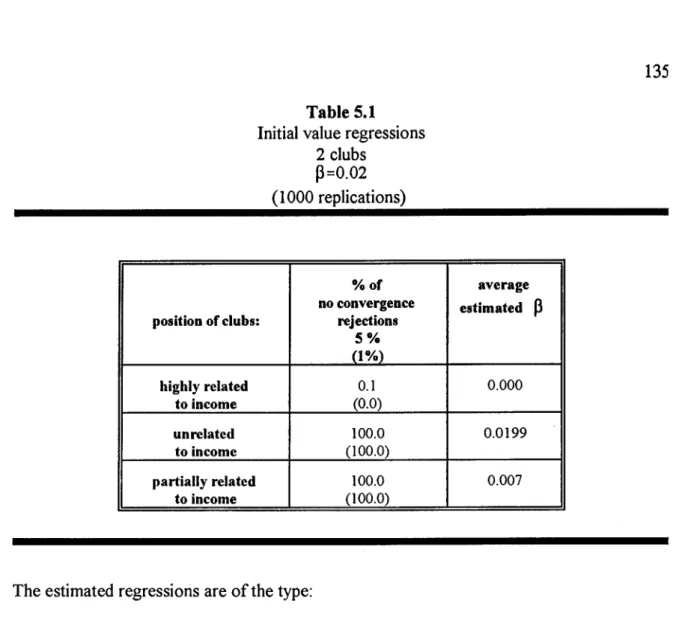
2. Misleading information from Barro-type and random field regressions, 134 3. Quandt tests, 13 6
4. Markov chains, 140
4.1 Position of clubs highly related to income, 141
4.2 Position of clubs completely unrelated to income, 142 4.3 Position of clubs partly related to income, 143
Conclusion, 144
Chapter 6. Limited Convergence, 146 Introduction, 146
1. Generating limited convergence, 146 2. Initial value and random field methods, 14 7
2.1 These methods are condemned to fail: theory, 147
2.2 These methods are condemned to fail: Monte Carlo evidence, 148 3. Identifying the convergence club, 150
3. 1 Markov chains methods, 150 3.2 Time series methods, 153 Conclusion, 154
Chapter 7. Time-varying Convergence, 155 Introduction, 155
1. The data generation process, 156 2. Time series methods, 157
2.1 Kalman filter method, 157
2.2 Augmented Dickey-Fuller tests, 159 3. Cross-section methods, 160
3.1 Initial value regressions, 160 , 3.2 Random field regressions, 164 3. 3 Markov chains, 166
Conclusion, 169
Chapter 8. Convergence Across Industrialised Countries (1890-1989), 171 Introduction, 171
1. The data set, 1 73 2. Convergence tests, 174
2.1 Dickey-Fuller and Augmented Dickey-Fuller tests, 174 2.2 Kalman filter tests, 176
a) The method, 176 b) The results, 178
2.3 Summary of results, 180
3. Estimating the speed of convergence and the steady-state, 181
3. 1 Estimates for the speed of convergence and the steady-state using OLS, 181
3.2 Estimates for the speed of convergence and the steady-state using the Kalman filter, 182
1.3 The period from 1890 to 1989, 183
3.4 Are the estimates stable through time?, 185 3.5 Convergence after the Second World War, 189 4. Initial value regressions reconsidered, 193
Conclusion, 195
Appendix to chapter 8, 197
Conclusion, 209
1. The starting point, 209 2. The aim of the thesis, 21 0
3. Main results and conclusions, 211
3.1 Evaluating methods for measuring convergence: results and conclusions, 211
3.2 Convergence across industrialised countries (1890-1989): the main findings, 214
Appendix. Some Gauss Routines Used in the Experiments Presented in this Thesis, 216 1. The data generation process, 216
2. Augmented Dickey-Fuller tests, 218 3. Initial value regressions, 221
4. Random fields regressions, 222 5. The Kalman filter, 223
6. Markov chains, 226
List of Tables
Chapter 2. Measuring Convergence: Methods and Results Table 2.1 Unconditional convergence results, 63
2.2 Comparing growth rates in different groups of countries, 64 2.3 Conditional convergence results, 67
8
2.4 Correlation of supply and demand shocks to the "central" country or region, 80 2.5 Percentage of variance explained by the first principal component for
geographic groupings, 81
Chapter 3. Unconditional Convergence
Table 3.1 Critical values for the T ( <I>~ML) statistic, 100 3.2 Ratio ofvariances (V1N 100}, 102
3.3 Nonparametric methods. Percentage of rejections ofthe no convergence hypothesis, 103
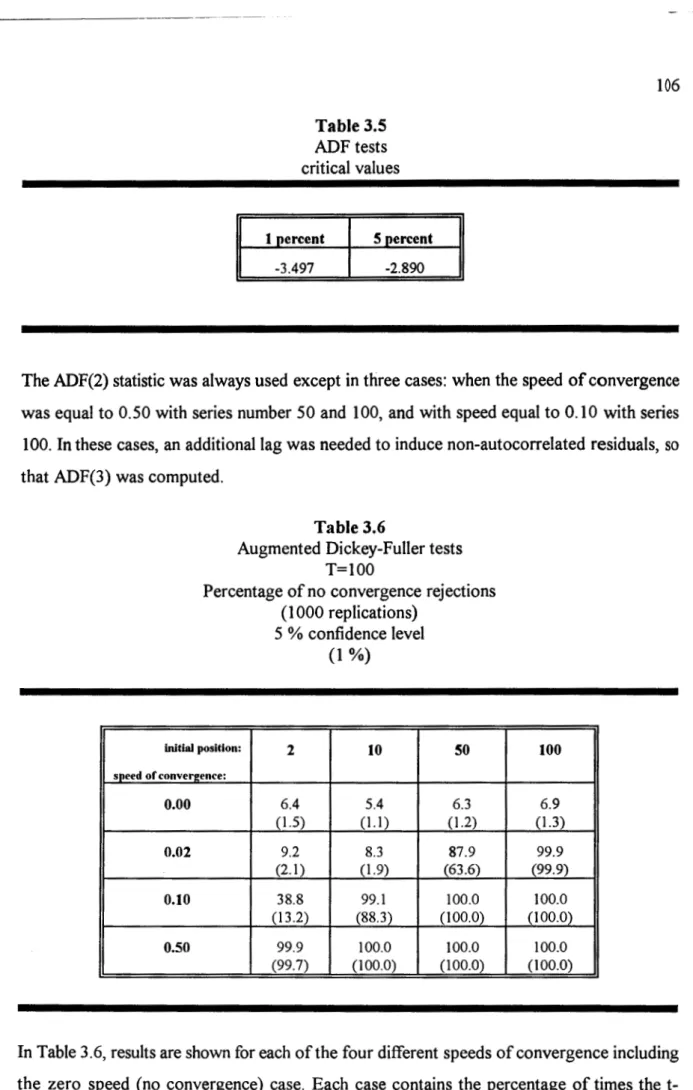
3.4 Initial value regressions, 105 3.5 ADF tests. Critical values, 106
3.6 Augmented Dickey-Fuller tests. T=100. Percentage of no convergence rejections, 106
3.7 Augmented Dickey-Fuller tests. T=40. Percentage of no convergence rejections, 107
3.8 Random field regressions, 108
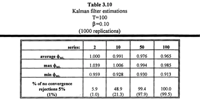
3. 9 Kalman filter estimations. T= 100. P=O. 02, 111 3.10 Kalman filter estimations. T=100. P=0.10, 112 3.11 Kalman filter estimations. T=100. P=0.50, 112
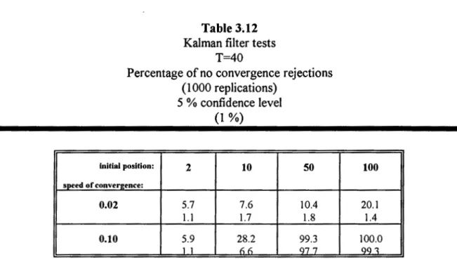
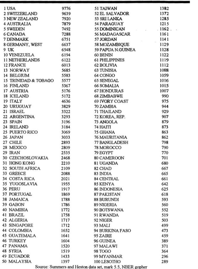
3.12 Kalman filter tests. T=40. Percentage of no convergence rejections, 113 3.13 Real GDP per head in 1960, 116
Chapter 4. Conditional Convergence
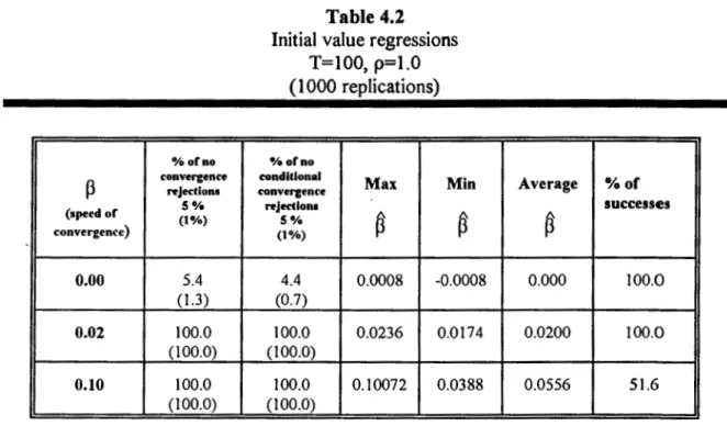
Table 4.1 Growth rates in real and artificial data compared, 122 4.2 Initial value regressions. T=100. p=l.O, 123
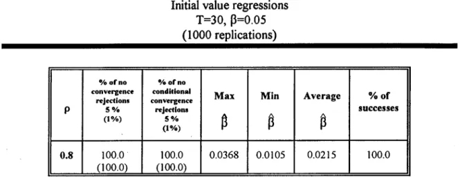
4.3 Initial value regressions. T=100. P=0.02, 124 4.4 Initial value regressions. T=30. P=0.05, 125
estimates. 1890-1989, 184
8.6 Steady-state as a percentage ofthe US. 1890-1989, 185
8. 7 Return to normality model. Unrestricted version. 1890-1989, 187 8.8 Steady-state as a percentage ofthe US. 1890-1946 and 1947-1989, 188 8.9 Speed of convergence estimates. 1950-1989, 189
8.10 Log-likelihood tests. Same speed and same steady-states across countries. 1950-1989, 191
8.11 Steady-state estimates. 1950-1989, 193
8.12 Steady-state estimates as percentage ofUS. 1950-1989, 193
8.13 Convergence to the US. Dickey-Fuller tests. Years with dummy variables, 197 8.14 Convergence to the US. Kalman filter tests. Years with dummy variables, 198 8.15 Dummies in the return to normality model, 199
8.16 GDP per head in the G-7 countries (1870-1989), 200
List of Figures
Chapter 1. The Importance of Convergence in Economics Figure 1.1. Savings and depreciation in a zero-growth model, 23
1.2. Savings and depreciation in a positive growth model, 24
Chapter 4. Conditional Convergence
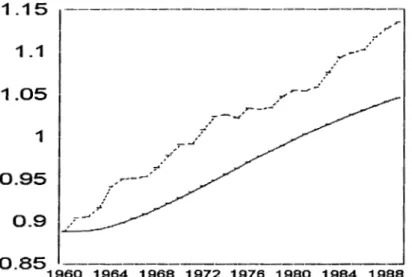
Figure 4.1 Standard deviation for artificial and real data, 121
Chapter 8. Convergence Across Industrialised Countries (1890-1989) Figure 8.1 Difference between Canadian and US GDP per head, 206
8.2 Difference between British and US GDP per head, 206 8.3 Difference between German and US GDP per head, 207 8.4 Difference between French and US GDP per head, 207 8.5 Difference between Italian and US GDP per head, 208 8.6 Difference between Japanese and US GDP per head, 208
Acknowledgements
I would like to thank my supervisor, Professor Stephen Hall, for his always invaluable and prompt advice.
I acknowledge financial support from JNICT (Junta Nacional de Investiga~ao Cientifica), Portugal, and The British Council.
Introduction
Convergence is an important issue in Economics. There is a convergence debate going on in growth theory. In international trade theory, it is possible to find the terms "convergence of prices" applied either to goods or factors. The word "convergence" is also found in the European Union economic and political jargon. This thesis is more focused on the growth theory debate, but its results are meant to be relevant from a more general point of view.
By convergence of incomes per head in growth theory it is sometimes meant a tendency for this or other similar variable to become more or less equal across different countries. In one important qualification, "convergence" is sometimes considered to be "conditional." In this case, GDPs or incomes per head do not converge to the same levels, but differences between countries become stationary, so that growth rates are the same in the long-run. This is a consequence of the neoclassical growth model, and some attempts have been made to directly estimate it. Also, some technological catch up models allow for the existence of a limited convergence outcome: only countries with the necessary social capability converge to the income path of a leader country.
In fact, different models in growth theory have different implications for convergence of income levels: endogenous growth models suggest a tendency for divergence of incomes. Growth rates usually depend on country specific parameters or policies.
The recent surge of endogenous growth models in growth theory that challenge the convergence properties of the neoclassical model was accompanied by an increasing number of empirical studies that directly address the question of convergence of incomes across different economies (being them countries, states or regions within a country.) These studies propose different methods to test and measure convergence, and results using the same or similar data sets are apparently in contradiction when different approaches are considered.
At the same time, empirical studies in other areas of Economics have dealt with the convergence testing and measurement issue. In international trade theory, the empirical validation of the "factor price equalisation theorem" has lead some researchers into testing for convergence oftime series of prices offactors. The Maastricht treaty on European Union and the convergence requirements contemplated in it have raised the concern in testing for
convergence of interest, exchange and inflation rates, and of budget deficits as percentage of the GDP across European countries.
The techniques used in different strands of the literature are not always the same, but due to the similarity of concepts involved, some of them can be considered as adaptable and may be used in different contexts.
The fact that results using different techniques applied to the same data set are in apparent contradiction was one of the main motivations for this thesis. It was felt that a deeper understanding of the properties of different methods of testing and measuring convergence was needed so that existing results could be correctly interpreted and new results could be obtained with more confidence.
No real data is used to evaluate the different methods. In its stead, their assessment is made by employing simulation techniques and different Monte Carlo studies are constructed to assess the various methods of testing for convergence. A typical experiment consists of the following steps:
1 -To generate several replications with several artificial series converging according to a pre-specified pattern of convergence (e. g. complete unconditional convergence or different convergence clubs.)
2- To apply different convergence tests and methods of measuring convergence to each replication and compute a number of statistics of interest (e. g. the number of times the "no convergence" null hypothesis was rejected.)
3 - To compare the performance of different methods under a similar convergence situation.
All the programmes used in these simulations were written on Gauss by the author and are available on request. A number of routines are included in an appendix to this thesis.
using real data was done, both to illustrate some of the points that arose from the experiments and to give a contribution to a the ongoing debate on convergence of GDPs per head.
The first chapter in this thesis ("The Importance of Convergence in Economics") starts with a definition of convergence that tries to encompass the often only implicit definitions that can be found in the literature. It then surveys the theoretical literature in Economics that deals with convergence, with an emphasis on growth theory, since most of the empirical results and methods resulted from growth studies and were designed to deal ~th the convergence of income levels across economies. Sections on the international convergence of factor prices and on nominal convergence in the European Economic and Monetary Union are also included.
The second chapter ("Measuring Convergence: Methods and Results") reviews the main techniques and their outcomes when applied to measuring convergence of real data sets. A first appraisal of the methods is made here, and some apparent contradictions in results (or "puzzles") are highlighted.
Chapter 3 to 7 present the different experiments and provide an evaluation of the different techniques under different types of convergence.
In Chapter 3 ("Unconditional Convergence"), the data generation process (DGP, for short) is "well behaved", in the sense that all the series converge at the same speed to the same leader series. In the long run all the series tend to the same level, except for a stationary disturbance. The DGPs in the following chapters are departures from this "good behaviour." This chapter also includes a presentation of the methods as they are considered in the experiments to come.
In Chapter 4 ("Conditional Convergence") the series converge to the same leader, but their long run difference is not necessarily zero. It is still true, though, that their long run growth rate is the same. This kind of framework is compatible, in growth theory, with the theoretical results derived from the neoclassical growth model. This simple departure from unconditional convergence already puts some strains on the performance of some of the considered techniques.
The DGP in Chapter 5 ("Convergence Clubs") imposes the existence of two groups of series that converge to two different leaders. This hypothesis is more or less explicitly dealt with by some of the techniques and these are assessed here.
Chapter 6 ("Limited Convergence") includes experiments where only part of the series converges to one leader. The other series do not converge at all. This is the theoretical outcome of some growth models like the ones based on the "technological catch up" idea.
Chapter 7 ("Time-varying Convergence") considers a situation where the different series only start to converge some periods after the "initial period." In practice, the researcher would like to consider the hypothesis that convergence starts to occur somewhere after the beginning of the available time series, without being able to exactly locate that period. An understanding of the properties of the different techniques of testing and measuring convergence is therefore needed to face this situation.
After the evaluation of the different methods, an empirical study is presented in Chapter 8 ("Convergence Across Industrialised Countries (1890-1989).") Here, some new findings are introduced concerning the convergence of fifteen industrialised countries incomes per head to the United States level using a century of yearly data1• This study makes use of the results
from the previous chapters.
The thesis ends with a general conclusion.
1
The countries considered are the Australia, Austria, Belgium, Canada, Denmark, Finland, France, Germany, Italy, Japan, the Netherlands, Norway, Sweden, Switzerland, the United Kingdom and the United States as a leader or benchmark country.
Chapter 1
The Importance of Convergence in Economics
Introduction: What is convergence of economic series?
The word convergence is often used with different meanings by different authors or in different papers. Quite often, there is no explicit definition of the id~a. One has to infer the underlying definition from the whole text. Of course, there are many convergence definitions in the statistical and mathematical literature. These are in some sense connected to the issue herein studied, and as it will be shown shortly, this is a source of some confusion.
Firstly, different fields of economic theory and practice that deal with this idea are briefly referred. Then some rigorous definitions of convergence thought to be appropriate for economic series are given. These definitions are believed to underlie an important part of the literature on the subject.
In growth theory, "convergence" usually means a tendency for poorer countries to catch up with richer ones through time, so that economic conditions become eventually more similar among economies. Usually, a single series summarises these economic conditions. Most of the times, the series is GDP per head or GDP per active person. The first section of the first chapter surveys the developments on convergence in the growth theory literature.
In international trade theory, it is possible to find the terms "convergence of prices" applied either to goods or factors. Usually, "convergence" is considered different from "full equalisation."1 "Convergence of international prices" would be observed if there is a tendency to a tightening of their distribution as measured by some dispersion measure. This chapter's second section deals with convergence of international factor prices.
The word "convergence" is also found in the European Union economic and political jargon. While the term "real convergence" refers to the growth theory meaning, "nominal
1
convergence" covers convergence in interest, inflation and exchange rates, and in budget deficits as percentage of GDP. This kind of convergence has a juridic expression in the Maastricht treaty. The third section in this chapter handles with this kind of issues.
The aim is to encompass all these meanings of convergence in a more general setting2, so that
measuring methods can have a sense without referring to specific series.
Consider two economic series
X.
and Y1• These two series converge_if:(1.1)
where E1 is a random variable obeying the following conditions:
(1.2)
and
(1.3)
Equations (1.1) to (1.3) mean that the difference between the two series converges in probability to a third series that is stationary, having a constant mean Dxy and a constant vanance a.
It should be clear that although
X.
converges to Y1 in economic terms, it does not convergein statistic terms. Nevertheless, a statistical meaning of convergence is used in the economic definition of the same term.
For reasons that will become apparent later, economic convergence is:
a) pointwise, if Var(e1)
=
0;b) unconditional, ifDxy = 0;
Ths follows an idea taken from Hall, Robertson and Wickens (1993). Here, the convergence definitions are somewhat different.
19 c) conditional, ifDxy =I= 0.
The definitions above encompass the "beta-convergence" concept proposed by Barro and Sala-i-Martin (1992a, 1995). In their work, series are assumed to converge to their steady-state level at an annual constant rate. If the steady-steady-states are the same, "beta-convergence" is unconditional. If they are different but grow at the same rate, "beta-convergence" is conditional. The definitions presented earlier in this introduction are more general because they do not imply a constant rate of convergence and therefore differences between series are not necessarily stationary from the beginning.
One possible formalisation of series that converge at a constant rate follows. It is one of the simplest forms of convergence but, with minor variations, it can be found in different theoretical models that predict convergence. It is also a good starting point for further extensions and it serves as an illustration for the different concepts of convergence previously defined.
Consider an attracting series X1 and n-1 attracted series denominated by ~ , with i varying
from 2 to n. The first series is a random walk with a drift:
(1.4)
where t is a time subscript.
The attracted series are generated according to:
(1.5)
so that they include an error correction term. In both equations E is a white noise random
variable, uncorrelated to previous values of x.
p
is the speed of convergence and is comprised between 0 and 1. d; is a series-specific constant.The difference between the attractor and any attracted series is therefore given by:
where 11 is the difference between the es. In the long run (as t tends to infinity) the difference between the series becomes:
d. = d +u
l,oo I ' (1.7)
where u depends on the 11s.
It can be inferred from equation (1. 7) that series i converges to series 1:
- conditionally, if d; is different from zero. In this case, the long run difference between the two series is a stationary random variable with a mean different from zero;
- unconditionally, if d; equals zero;
-point wisely, ifthe variance of the es, and consequently of11, is zero.
For some authors, convergence means a tendency for the cross-section dispersion of series to diminish over time. This concept is called "sigma-convergence" by Barro and Sala-i-Martin (1992a, 1995)3. It is shown below, using the same example, that convergence according to the earlier definition does not imply "sigma-convergence."
If the long run difference d; is added to each attracted series, the resulting "parallel" series converges unconditionally to series 1 and is given by:
The cross-sectional variance of X;,r c is equal to:
Noting from equation (1.8) that X;,~ does not depend on d; and recalling that:
c -x., I,
=
x1.,-d., , I (1.8) (1.9) (1.10) 30therexamp1es of the use of this definition are Tovias (1982), Baumo1 and Wolf(l988), Mokhtari and Rassekh (1989) and Lichtenberg (1994).
it results that:
(J 2
=
(J 2 + 02Xt X
.,
d' (1.11)Using (1.9) and (1.11), it can be concluded that:
(1.12)
In the long run, the cross-section standard deviation is equal to:
2 1 2
(J
=
CJ-+ (JX d P(2+P)' € (1.13)
depends
The long run cross-section variance positivel/on the variance of the shocks that affect each economy and also on the variance of
d .
This last variance reflects the variation in the different steady-state levels. If convergence is point wise and unconditional, both these variances are zero and the cross-section standard deviation becomes also zero, so that all series coincide precisely.From equation (1.12), and taking into account that
p
is comprised between 0 and 1, it results that a declining or increasing time path fora
x,
2 are both compatible with any ofthe definitions of convergence (conditional or unconditional.)a
2 declines through time if itx,
starts from a value higher than its long-term mean, and conversely, will increase if the series start too close together. For example, in case of unconditional convergence, if the series start all at the same point, the cross-section variance is expected to increase, driven by the cumulative effect of the series-specific random shocks.
1. Growth theory and convergence
1.1 The neoclassical model without growth
Solow (1957) neoclassical growth model remains a useful reference for the understanding of more recent developments on growth theory and convergence. In its simplest version, the Solow model exhibits no long run growth. In the steady-state, income and (physical) capital
per head remains constant. Most neoclassical or endogenous growth models surveyed in this review are better understood as departures from this simpler model. It is therefore important to identify the hypotheses that impede long run growth here, since at least one is usually dropped in the other models.
Production at a given time (Y) depends on capital (K) and labour (Lt, A being a country specific constant:
Y
=
AF(K,L). (1.14)This function (sometimes called the "neoclassical production function") is supposed to be homogeneous of degree one, twice differentiable and to obey the following conditions:
F2(K,L)>O, Z=K,L, FKL (K,L) =FLK(K,L )>0, FKK(K,L )<0 and FLL (K,L )<0, lim F2(K,L)=+oo,
z-o
lim
F
2(K,L )=0, Z-oo Z=K,L. Z=K,L, (1.15) (1.16) (1.17) (1.18) (1.19)meaning that marginal productivity is positive but decreasing to zero, being infinitely high when the factor is used in very small quantities. Conditions (1.18) and (1.19) are called the lnada (1963) conditions.
Since the production function is homogeneous, production per unit of labour depends on capital per unit oflabour5:
4
Time indexes are dropped when they are not necessary.
5
y
Ky
=
L=
AF(L,1}=
Af(k). (1.20)Iflabour grows at an exogenous rate n and capital depreciates at a fixed rate 5, then the law of motion for capital is:
k =sAf(k)-(n+i>)k, (1.21)
where the savings rates is constant6
• A variable with a"." stands for its time derivative.
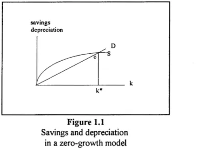
Figure 1.1 represents equation (1.21}. In that graph, curveS depicts savings as a function of capital per head (sAf(k)) and lineD pictures capital per head depreciation ((n+i>)k).
savings depreciation
k*
D
Figure 1.1 Savings and depreciation
in a zero-growth model
k
Since the marginal productivity of capital tends to zero, the slope of curve S is decreasing and zero in the limie. Consequently, it crosses lineD at some point c. Net investment is equal to the difference between S and D. To the left (right) of k'", capital per head is increasing (decreasing) so that k* is a stable equilibrium.
It can easily be concluded that this model only exhibits growth as part of its transitional
~e saving rate could be endogenously detennined by some kind of optimising behaviour. The issue here
is to make the hypotheses that impede growth explicit. As it will be apparent soon, these come from the production function specification and do not depend on consumers behaviour.
7
dynamics: capital per head and therefore production grows while they are lower than their long run (steady-state) value. Once that point is reached, there is no room for additional growth.
The following two hypotheses may be shown to be responsible for this result:
i) A is constant;
ii) the marginal productivity of capital tends to a value inferior to (5
+
n)/s.Suppose that A increases through time. The marginal productivity of capital would not fall to zero, and capital per head could be accumulated indefinitely. In graphical terms, this would correspond to successive upward shifts in the S curve. This is the solution adopted by the exogenous growth neoclassical model, but also by several endogenous growth models.
savings depreciation s D k Figure 1.2 Savings and depreciation in a positive growth model
Otherwise, consider that the marginal productivity of capital does not fall to zero, but tends to some positive quantity that is higher than (o
+
n)/s. Now, capital marginal product is asymptotically constant and positive and net investment is assured to remain positive. Net investment translates itself directly into growth. In graphical language, this means that curve S has a limiting slope that is higher than 5 + n, and never crosses line D. Figure 1.2 pictures this situation. As it will be shown later, a family of endogenous growth models rely on this kind of assumption.1.2 The neoclassical model with exogenous growth
a) Optimising approach
As previously explained, growth can be introduced into the neoclassical model if it is assumed that A grows through time. This was Solow's approach in his 1957 paper. That kind of exogenous technical progress may be combined with optimising consumer behaviour, as done by Koopmans (1965).
Most writers use the same intertemporal utility function8, maximised by a representative consumer, be their models exogenous or endogenous growth ones. Apparently, this revealed preference derives from the functiommathematical tractability. Some authors want to have their work compared with previous theoretical research, and this seems to contribute to the persistence of this use9. Some important insights would remain clear if, say, constant saving
rates were assumed. This robustness of results is comfortable since it minimises the possible biases that could result from the arbitrary choice of a preferences pattern. Having written this, the tradition is followed and the neoclassical model is presented with exogenous technological progress and optimising behaviour.
The version that is presented below is the one used by Barro and Sala-i-Martin (1992a, 1992b, 1995) and also by King and Rebelo (1993) with minor differences. Chiang (1992) contains a succinct and clear mathematical explanation of the model.
The production function is the neoclassical one, but this time
A.
is not constant and represents the labour augmenting technological progress, its growth rate being denoted by g:(1.22)
(1.23)
8
Among others: Barro and Sala-i-Martin (1992a, 1992b, 1995), Chiang (1992), Helpman (1992), King and Rebelo (1990, 1993), Lucas (1988), Rebelo (1991, 1992) and Romer (1990a).
9
As before, labour is supposed to grow at the constant rate n:
(1.24)
It is useful to divide both terms of equation (1.22) by
Al-.-t,
to get a production function in "per unit of efficient labour'' terms:y
Ky
= -
=
F ( - 1)=
f(k).AL AL' (1.25)
where small letters refer to per unit of efficient labour variables and time indexes are omitted.
The resource restriction may be expressed in per unit of efficient labour terms, as follows:
k
=
f(k)-c-(g+n+3)k. (1.26)The representative consumer is supposed to maximise the following intertemporal utility function:
oo (C/L)r-6
U=f
r r L e nte -utdt.1-8
°
0
(1.27)
The momentary utility function exhibits constant marginal utility elasticity (8). The representative consumer cares about consumption per head, weighted by population size. u is a discount factor. It is possible to write the utility function in terms of per efficient unit of labour consumption ( c,). It can be shown that:
00 c l-6
U=LaAd
-6J
_r_e (g+n-g6-u)tdt. 01-8
(1.28)
To simplify, U is divided by L0Ao(l-8). The resulting utility function V is a monotonic transformation ofU, and therefore represents the same preferences:
00
c
1-0V =
J -
1- e
-ptdt.o
1-e
(1.29)
p is a discount rate that is assumed to be positive and that depends on other parameters:
p=u+gf)-g-n (1.30)
It is possible to show that a representative consumer that maximises V will choose a consumption path that obeys the following:
c
=
e-l(r-p),c
(1.31)
where r is the real interest rate. Here, the relevant interest rate is equal to the net marginal productivity of capital:
(1.32)
Equations (1.26) and (1.31) describe the time path for consumption and capital and are therefore crucial to derive the steady-state and to describe the transitional dynamics.
When the economy is in the steady-state, capital and consumption per unit of effective labour remain constant. In algebraic terms, this means that the two following conditions hold:
c
= 0t ' (1.33)
k = 0
t ' (1.34)
From now on, the production function is assumed to be Cobb-Douglas, so that:
and
y
= f(k) = ka.. (1.36)The steady-state values for capital (k*) and consumption ( c*) per unit of efficient labour are accordingly derived from equations (1.26) and (1.31), using (1.30), (1.32) and (1.36):
(1.37)
(1.38)
In the steady-state, consumption per capita and capital per capita grow at the same rate g, which happens to be the rate of technological progress.
Equations (1.26) and (1.31) are non-linear differential equations. One way to analyse consumption and capital behaviour close to the steady-state is to log-linearise these equations around it.
Applying logs to both equations results in:
(1.39)
(1.40)
Equations (1.39) and (1.40) can be rewritten as:
logk
=
e<cx-l)logk_elogc-logk_{g+n+o). (1.42)In the steady-state, log c and log k remain constant. The following expressions are useful when deriving the results that follow them:
( 1)1 k • g+n+o+p
loge = 0 - e ex- og = .::::,__ _ _,:_
a
lo~k
=
0 _ e loge• -logk•=
(1-a)(g+n+o)+pa
(1.43)
(1.44)
The derivatives that follow are evaluated at the steady-state and derived from (1.41) and (1.42), using (1.43) and (1.44): a loge alogk alogk
a
loge a loge a loge=
0,= _
(1-a)(g+n+o+p)e
_ (1-a)(g+n+o)+p alogk aiogk=
p. (1.45) (1.46) (1.47) (1.48)The log-linearised system is as follows:
(
lo~e)
= (
0 logk-Jl2
-Jl•)
(loge -loge•J
P logk -logk • where:a
loge,Jll
=
alogk,' andThe system matrix eigenvalues are A1 and A2:
Accordingly, the law of motion for capital is:
atogk,
a
loge, (1.49) (1.50) (1.51) (1.52) (1.53) (1.54)Noting that
A
1 <0 but thatA
2>0 , it is necessary to set 112=0 to rule out any explosivebehaviour that would violate the transversality conditions. The value for 11
1 results from the initial condition:
111
=
logk0 -logk •.The solution for log k1 is derived using expressions (1.54) and (1.55):
~ t
logk, = logk • +(logk0 -logk *)e 1 •
(1.55)
(1.56) Since
A.
1 is negative, it is clear from equality (1.56) that k, approaches k* asymptotically.Noting that y,=k,«, it follows that y increases (or decreases) at the same rate ask:
~ t
log y1
=
log y • +(log y0 -log y *)e 1 •Expression (1.57) can be transformed into the following:
logy, -logy0
t
This last equation shows that:
=
1 -e ~ 11 1 -e A-11 - - l o g y0 + logy •. t t (1.57) (1.58)- the time average of income per unit of effective labour growth rate tends to zero over time;
- the time average of income per unit of effective labour growth rate is higher the smaller initial income is.
Recalling that:
(1.59)
it is also possible to write an equation for the average growth rate of income per head, using (1.58) and (1.59): Y, Y0 log- -log-L, L0 t (1.60)
The average growth rate of income per head approaches g, the rate of technical progress, as time tends to infinity. The average growth rate is the higher the lower initial income is.
Convergence properties of the neoclassical model
To assert the type of convergence that this model exhibits one can suppose that two countries share the same rate of exogenous technological progress g. After both have converged to the steady-state, both countries' income per head grow at the same rate g. This is already apparent from equation (1.60), but it is useful to derive an expression for income per capita once the economy reached the steady-state.
Income per head is given by the following equation, which is derived from the production function:
In the steady-state, capital per unit of labour is:
Substituting (1.62) into (1.61) it gives:
K
=
Ak*. L(1.61)
(1.62)
(1.63)
Let two countries be named A and B. Country A income per unit of labour relative to B is constant and equal to:
Ya -A k*"' La o,a a
=
yb *"' Ao,bkb (1.64) LbSo equation (1.6+) shows that even if two countries share the same production function, preferences and rate of technical progress (so that their steady-state capital per effective unit oflabour is the same), they do not necessarily tend to the same income per capita, since they may well have different Aos. Since their incomes will grow at the same rate, the logs of their
incomes will differ by a constant.
Moreover, even if two countries share the same rate of technical progress, they tend to grow at the same rate g, so that the proportion between incomes per head stays constant,
even
if
all the other parameters are different.
This means that, in general, the referred model assures
conditional point wise convergence
between (logs of) incomes per capita. The constant will be a function of initial conditions and preferences' parameters. It is of course possible to introduce some stochastic elements in the model in order to get a conditional convergence result that is not point wise.
b) A neoclassical model that includes human capital
Mankiw, Romer and Weil (1992) is an influential paper that, in its authors' words (p. 407), "takes Robert Solow seriously." It is an attempt to show that (p. 407) "an augmented Solow model that includes accumulation of human as well as physical capital provides an excellent description of the cross-country data."
Production level is supposed to depend on three factors: labour (L ), physical capital (K) and human capital (H), the production function being Cobb-Douglas:
(1.65)
where, as before, A stands for the level of technology, progressing at a rate g, and L grows at a rate n.
This model does not include any utility maximization. Instead, investment in human and physical capital is constrained to be a fixed proportion of income, B being the common depreciation rate:
(1.66)
As before, small letters refer to quantities per effective unit of labour.
The implied levels of steady-state human and physical capital are:
( 1-P p ) 1
s
s
-k *
=
k h 1-cx-p, n+g+o andApproximating around the steady-state:
dlogy
- -1
=
A(logy*-logy1),
dt
where
A
(the speed of convergence to the steady-state) is given by:A=
(n+g+o)(I-a-p).This result implies the following one:
(1.67) (1.68) (1.69) (1.70) (1.71) (1.72)
The similarity between this last result and the one derived from the model without human capital is complete (see equation (1.57)), except for the concrete value of A. However, Mankiw, Romer and Weil prefer to substitute for the value ofy* and derive the following "initial value" expression:
logy,-logy0 = (l-e-l1) a Iogsk+(l-e-l1) P logs~z-(1-e-l1)~log(n+g+o)-(l-e-l1)logy
0
1-a-p 1-a-p 1-a-p
(1.73)
Growth of output per effective worker depends negatively on initial income, but the respective coefficient tends to 0 through time. It is worth noting that growth also depends on the saving rates and on the rates of population growth, technical progress and depreciation.
Following the same lines as done previously with the model without human capital, it can be shown that:
- when t tends to infinity, countries exhibit the same income per head growth rate; - when transitional dynamics are still operating, per head income growth rate depends negatively on initial income and on the determinants of the steady-state, very much like the last equation shows.
It can therefore be concluded that both neoclassical models imply some sort of conditional convergence i.e. convergence of incomes per capita after conditioning on a set ofvariables that allow for steady-state differences.
1.3 Convergence and technological catch up: a non neoclassical approach
Several authors have given some explanations and developed theoretical arguments for levels ofGDP per head convergence. These come either as a justification for an observed empirical pattern (especially among the OECD countries) or as a testable hypothesis.
An influential paper by Baumol (1986) provides empirical evidence in favour of convergence among OECD countries and of divergence of larger groups of countries, thus conducing to the idea that there is a "convergence club." His econometric methods will be surveyed later. Convergence is considered to result from the international public-good nature of successful productivity-enhancing measures. On the one hand, countries increasingly imitate innovations. On the other hand, investment also may exhibit international public good properties, even if the factor price equalisation theorem is not applicable.
Abramovitz (1986) provides the notion of"social capability": different social institutions and processes make some countries better or worse at catching up. Accordingly, some forge ahead while others fall behind.
There is an important difference between these explanations for convergence and the ones that come from neoclassical models. The latter usually assume the same rate of technological progress in every country (at least the ones that belong to the same club), convergence being explained by the accumulation of capital conditioned on possibly different steady-states. The
reader can think of the former as models in which each country exhibits different rates of technical progress, the converging or catching up countries having a higher growth rate than the technological leader.
Dowrick and Gemmell (1991) emphasise that catching up effects may differ across sectors (agriculture and industry, for instance) and across countries. Moreover, differences in GDP growth rates may also result from different growth rates of factor inputs.
Dowrick and Nguyen (1989) formalise this last point. Country i output at time t is supposed to obey the following equation:
(1.74)
where y is the leader's rate of technological progress (the rate of growth in "total factor productivity" in the leading country),
A.
is a positive parameter smaller than one and F~t is a catch up function, defined as:Y!,t-! F;,t _ L!,t-1 - - - , F;,r-r ~.t-r (1.75) L; r-r
where country 1 is the leader. From these, Dowrick and Nguyen (1989) derive the following:
Y. y!
I I, t I ,t
o g - - o g -
=
Li,t LI,t
where ~ and li stand respectively for the constant capital and labour growth rates in country
I.
From this last equation results the following expression for the "final year" relative output per worker:
If one takes the limit of expression ( 1. 77) as time tends to infinity, it results that:
(1.78)
From expression (1.78), it can be concluded that the difference between the logs of incomes per capita tends to a constant. This constant depends on the relative growth rates of capital and labour.
The average growth rate of income per unit oflabour can be shown to be equal to:
where and 0
=
1-(1-J..l T (1. 79) (1.80) (1.81)Since J..>O the average growth rate of a country income per capita depends negatively on the initial income value. The coefficient approaches zero as time goes by. This is not without a parallel with the results from the neoclassical model. Also note that the average growth rate approaches the growth rate of the leading country as time tends to infinity. In fact, it happens that:
lim gYIL- = y +ak1+(P-l)l1.
T-oo I
(1.82)
It can be concluded that two different countries end up growing at the same rate as that of the leading country, so that the logs of their incomes will differ by a constant. The model implies a form of conditional convergence, allowing for some transitional dynamics. Convergence is point wise, because there is no stochastic element. This result is very similar to the ones derived from the neoclassical models discussed before.
1.4 Endogenous growth models10
a) Growth and returns from capital
As previously discussed, a main obstacle to growth in the simple neoclassical model is the decreasing returns to capital and their tendency to a quantity that is sufficiently close to zero.
If returns to capital are decreasing but do not tend to zero, it is possible to have endogenous growth (meaning that the growth rate depends from the model parameters values.) Jones and Manuelli (1990) model exploits this idea. The implied production function is of the type:
a 1-a
Y,
=
AK, +BK, L, . (1.83)Since it does not affect the relevant results, one can assume that labour is constant (make it equal to one) and that there is no depreciation.
Clearly returns to capital tend to A, supposed to be a constant. In the long term, the time change of capital is:
K
=
sY=
sAK. (1.84)where sis the savings rate. It can be concluded from (1.84) that the long term growth rates of capital and income are both equal to:
K =sA. K
(1.85)
This long term result is obtainable even in the short term with the simpler linear production function (the so called "AK" function):
Y,
=
AK,. (1.86)That was the approach made by King and Rebelo (1990). The savings rate is endogenously determined by means of a representative consumer maximising a utility function similar to (1.27). However, the fixed savings rate assumption is enough to show that it is the different
10
Sw-veys of endogenous growth literature include Barro (1995), Boltho and Holtham (1992), Hammond and Rodriguez-Clare (1993), Romer (1991) and Verspagen (1992).
technology that is responsible for the.endogenous growth result.
If a representative consumer maximises an intertemporal utility function as the one expressed in (1.29) and considering that here it happens that
r=A,
it can be shown that11:r
=
c
=
K
=
e-•cA-p).Y C K
Two features of the AK model are worth noting:
(1.87)
- There are no transitional dynamics. Adjustment to a change in, say, the savings rate, is immediate. If savings increase as a proportion of income, the growth rate adjusts immediately and permanently to its higher level.
- This model can be seen as the limit of the neoclassical simpler model, when
a
approaches unity.None of these models imply convergence of any kind. If two countries have different technologies (different As) or different saving rates (because of different preferences or different tax policies), they will not converge. On the contrary, they will display permanent differences in their growth rates.
b) Growth as a side effect of other activities
A number of authors have developed models that can be classified under this heading. To make the algebra simpler, consider a Cobb-Douglas production function ofthe form:
Y = O.Ka.(A L )1 -a.
t t t t ' (1.88)
where Q is a constant. Labour is supposed to grow at the rate n. Consider that capital does not depreciate and is accumulated from foregone consumption according to a function G:
K
=
G(Y-C,K). (1.89)11
Growth will be seen to result either from the accumulation of capital, from an endogenously determined learning process or from the enhancing productivity qualities of public goods. These different engines of growth will translate themselves into different formulations for ~·
Growth as a side effect of the accumulation of capital
Technical progress is seen as a consequence of the accumulation of capital, according to the following expression:
A,
=
K,11• (1.90)The economic justification of this last expression is different across authors, as it will become clear soon.
P1
case: 0<11 <I.
This is the original formulation of Arrow (1962) and Sheshinski (1967). According to the latter author (p. 33), "~is assumed to reflect accumulated experience in the production of investment goods." The function G is taken to be simply as G=Y-C. Substitute expression (1.90) into (1.88) take logs and differentiate, to get:
logY= [cx+11(1-cx)]logK+[l-cx]logL. (1.91)
Note that the production function displays increasing returns to scale, but decreasing returns to any of the factors. There is a unique growth rate that assures that capital and income grow at the same rate:
. . n
logY = logK =logY = - - .
1-11 (1.92)
This model has the inconvenient property that makes growth depend on the rate of growth of population. If population growth is zero, we are back to the neoclassical simpler model. Nevertheless, it exhibits an interesting departure from the neoclassical framework: returns to
scale are not constant, so that payments to factors according to marginal products do not sum up to total income. Consequently, private decisions drive the economy to a sub-optimal equilibrium, as shown by Sheshinski (1967). Since the next case is a more radical departure from neoclassical assumptions, this one will not be further discussed.
2nd case: 11
=
1.This case is developed by Barro and Sala-i-Martin (1992c) and is inspired in Romer {1986). As before, G=Y-C. Population is supposed to be constant, or, more precisely, this is a per capita model. The interpretation of~ differs from Arrow' s. Here, it is supposed that:
(1.93)
where Ka,t is the average level of capital used by other producers. Substituting {1.93) into (1.88) the production function becomes:
(1.94) In its original formulation by Romer (1986) K represents accumulated knowledge, or a composite capital good that includes knowledge and physical capital. Each firm observes decreasing returns to its own level of capital but returns remain constant to the total level of
capital. This formalization allows for the existence of a competitive equilibrium that is not Pareto optimal. The private return to capital is equal to:
(
K )
t-a:
r = aQ .; = aQ, (1.95)
where it was considered that K=Ka. It is not difficult to notice that we are back to the AK model, with A=Q. Accordingly:
Y
=
C=
K=
e-t(aQ-p).Y C K
(1.96)
Ifthe social return to capital (equal to Q) was considered, the optimal growth rate would be higher and equal to:
Y
=
c
=
K=
e-l(O-p).Y
C
K
(1.97)
When private agents make their decisions, they do not take the external benefits of their investment programmes into account. This is the reason why the competitive equilibrium growth rate falls short of the social optimum one.
This is the case that corresponds to the original Romer (1986) formulation. Aggregate returns to capital are supposed to be higher than 1. The function G(l, K) is assumed to be concave and homogeneous of degree one, so that:
·
(Y-C)
K
=
G(Y-C,K) = K g / ( . (1.98)Romer imposes two other restrictions on g. The derivative function of g obeys the restriction g'(0)=1, and, more important, returns in research are strongly decreasing so that g is limited from above:
Y-C for all--.
K (1.99)
This condition assures that the rate of growth of the state variable K remains bounded and therefore allows for the existence of an optimum.
In general, this formulation can produce ever increasing growth rates. Furthermore, growth rates may well depend on the size of the country, so that bigger countries grow faster. This model also displays the already discussed edge between social optimal and competitive equilibrium growth rates.
Growth as a result of learning by studying
In his 1988 paper, Lucas presents two endogenous growth models where growth results from a labour augmenting technical progress that derives either from endogenous decisions on
studying or from learning by doing.
Suppose that individuals spend a proportion u of their time working, ( 1-u) being time spent in studying. Their productivity increases in proportion to time spent studying:
A, = A,<j>(I-u,), (1.100)
There <I> is a constant. Note that
u.
is a choice variable. Under the maximisation of the usual intertemporal utility function, the balanced growth path will result in a growth rate that is equal to12:y
y
CC
=
KK
=
e-'(<j>-p). (1.101)This result is similar to the AK model growth rate. Nevertheless, this model is more complex due to the existence of two state variables (A and K), so that transitional dynamics are at work.
Lucas (1988) first model is a bit more complex. It involves an externality that arises from the learning process. The complete model production function is:
(1.102) with A\ reflecting this hypothesis. As expected, this externality leads to the conclusion that the market economy will display a lower growth rate, since people will study "less than they should," not considering that their own skill is the other's catalyst.
Growth as a result of learning by doing
The reader may be that rather practical man that thinks people learn more on the job than at school, and that studying is more properly assigned to leisure and has no productive impact. In that case, the previous model is easily modified to fit this alternative specification.
Let:
12
A,
=
A,<!>u,,
(1.103)so that labour productivity increases with time spent on the job and not on leisure activities. The algebraic results would be much the same.
Lucas (1988) follows this idea in a second model that has the interesting variation ofbeing a two goods and more than one country framework. Its main contents are sketched below.
There are two goods in the world economy: a high technology and a low technology one. Production functions are equal across countries and supposed to be Ricardian ( labour is the only factor.) The high technology good production displays a higher learning by doing potential (meaning a higher
"<I>"
in terms of equation (1.1 03)).If the economies that compose the world economy are open ones, countries will completely specialise in the production of one of the goods. If the goods are good substitutes, Lucas show that countries may find themselves stuck in the production of either high or low technology goods, according to the initial conditions. Due to the lower learning by doing potential of low technology production, low technology countries will grow less than high technology ones.
Growth as a result of the provision of public goods
Barro and Sala-i-Martin (1992c) include three models that can explain growth as a result of the public provision of public goods or services. These are productive inputs to private producers. One model considers public services that are rival but excludable. Another allows for congestion of the public services. The one sketched here treats public services as non-rival and non-excludable. Formally, they are much alike.
Regard labour as constant at the unit value and let:
A,
=
G,, (1.104)'t:
(1.105)
Private agents take the level of public services as given, so that the interest rate is equal to:
(
K)
1 -(Xr
= (
1 -,;)ex Q G . (1.106)Some algebra permits to derive the following expression for r, from expressions (I. 1 05) and
(1.1 06):
1 1 -IX
(1.107)
This comes to be another rationale for the "AK" model, with A=r defined as above. Ifthe consumer is maximising the usual utility function (as in Barro and Sala-i-Martin (1992c)) income, capital, public services and taxes all grow at the same rate:
Y = G = T = K =
e -
1 (r _ p ).Y G T K
(1.108)
The reader is probably looking for the externality included in this model. It derives from the fact that private agents underestimate the marginal productivity of capital, not considering that an increase in production means an increase in taxes and in the provision of public services. The higher level of public services acts as an effective counterweight to a decreasing productivity of capital. As usual, the "social planner" growth rate is higher.
c) Growth as a result of profit induced R&D
The first group of endogenous growth models previously presented were either straightforward modifications ofthe neoclassical model, as is the case of the "AK model," or models that display growth as a kind of by-product. All of them deliver important if partial insights.
In the former case, it can be argued that endogenous growth is technically delivered without a convincing economic structure or explanation behind it. Decreasing returns to each factor
combined to constant returns to scale are compatible with a perfectly competitive economy. No wonder then that the following question is: is there an alternative economic structure that produces results that fit with an aggregate function equal or close to the "AK" one? One attempt to solve this was made by Romer (1986). He showed that a competitive equilibrium may well coexist with aggregate non decreasing returns if some externalities are at work. Some years later, the same author (Romer (1990a)) and other writers (Helpman (1992), Barro and Sala-i-Martin (1992c)) developed models that settle the problem by dropping the perfect competition hypothesis and adopting a monopolistic competition layout.
All the aforementioned contributions make growth endogenous by explicitly introducing a research and development sector that is profit motivated. Some of these authors13 refer to a come back to Schumpeterian ideas of creative destruction. This is an important difference from all models considered until now, from a formal but also explicative point of view.
In these models the R&D sector either produces designs of new goods or factors or improves the quality of existing ones. The new or improved factors or goods result in economic growth. These two cases are formally quite close but will be treated separately.
Increasing product or factor variety
Barro and Sala-i-Martin (1992c) model may be seen as a restriction of Romer (1990a). Helpman (1992) and Romer (1990a) are variants of the same idea. This allows for a common exposition that will highlight the main ideas and differences of these approaches.
The production function for final goods is:
y
=
HIXLI-a.-pfN, .Pd·r y,r r x,,r 1,
0 (1.109)
where Hy,t is the amount ofhuman capital used in the production of final goods, L1 is the amount of labour, and ~~ is the amount of producer durable i. It is assumed that there is a continuum of durables, its number being N,. Barro and Sala-i-Martin consider a restricted
13
version of(1.109), with Ry=l and a=O. Helpman14 considers the case where Ry=L=l.
Durables are produced from forgone consumption15, so that:
K -t - 11
JN'
o Xl,t I . d"The usual resource restriction applies:
K,=Y,-Cr
(1.110)
(1.111)
Labour and human capital are constant over time. The last may be used in the production of final goods or in the R&D sector:
(1.112)
Suppose that each durable is used in the same quantity, irrespective oftime:
Xi,t
=
X. (1.113)If(1.113) holds, the production of final goods is equal to:
(1.114)
Using (1.110) and (1.113), it is possible to substitute for N, in (1.114) and get:
Y t
=
11 Hct y,t L I-ct-P -p-IK X r (1.115)Here is the "AK" model again. IfK grows at a rate g, Y will grow at the same rate, iflly and L stay constant. In other words, there is a balanced growth possibility for this economy. The market structure that supports this path in the steady-state is described next.
1
'1-lelpman (1992) considers Y to be an index defined in terms of varieties ofhigh-tech products, but this index can easily be reinterpreted as a final good produced by means of varieties of high-tech inputs.
1~elpman's version is somewhat different, durables being produced according to a Ricardian production function.
The constant returns to capital result means that there is no perfect competition solution for this model16
• Instead, a monopolistic competition framework will be adopted.
Consider an economy divided into three sectors: final goods production, production of durables and research and development.
The final goods sector produces according to the production function ( 1.1 09). Note that this function implies that the elasticity of substitution between each pair of durables is constant and equal to ( 1-p)-1• Demand for durables functions have constant elasticity so that marginal
revenue MR(i)=Pp(i).
There is only one firm that produces and sells durable i. Monopolistic pricing means that marginal revenue is set equal to marginal cost. The marginal cost of producing durables is equal to li}, r being the interest rate. A symmetry argument make it possible to conclude that prices for each durable are equal:
(1.116)
If r is constant in time, the price p and quantities x will also be invariant in time. The operational profits are the same across firms and through time and equal to:
(1.117)
Each firm buys the design for its durable from the R&D sector. In this sector, designs for durables are produced by means of human capital only, N, being the number of designs produced till time t. It is assumed that:
(1.118)
The marginal productivity of human capital equals oN, and therefore increases linearly with N,. The more designs have already been invented until today, the more are going to be
16