A NALYSIS OF AC REDITR

M

ASTER

A

CTUARIAL

S

CIENCE

M

ASTER

´

S

F

INAL

W

ORK

D

ISSERTATION

D

EFAULT

R

ISK

:

A

NALYSIS OF A

C

REDIT

R

ISK

M

ODEL

R

ICARDO

M

IGUEL DO

B

RITO

P

ENHA

M

ASTER

A

CTUARIAL

S

CIENCE

M

ASTER

´

S

F

INAL

W

ORK

D

ISSERTATION

D

EFAULT

R

ISK

:

A

NALYSIS OF A

C

REDIT

R

ISK

M

ODEL

R

ICARDO

M

IGUEL DO

B

RITO

P

ENHA

S

UPERVISION

:

M

ARIA DE

L

OURDES

C

ENTENO

i

A

CKNOWLEDGEMENTS

Quero primeiro agradecer à instituição bancária que disponibilizou os dados utilizados neste trabalho. Às pessoas que me acompanharam mais de perto, um muito obrigado por toda a preocupação que demonstraram e ajuda nas dúvidas colocadas.

À minha orientadora, Professora Doutora Maria de Lourdes Centeno, uma palavra de gratidão por se ter disponibilizado sempre em ajudar. Pelos valiosos conselhos e críticas construtivas, o trabalho pôde tomar um rumo melhor.

Tenho também muito a agradecer à minha família: pais, irmãs e avós. Aos meus pais em especial, por terem sempre criado condições para que este trabalho, e todo o restante percurso académico, tivesse sucesso.

Aos meus amigos, em particular ao Aires, João, José, Lourenço e Tomás. Muito obrigado por todo o apoio.

ii

A

BSTRACT

A considerable part of the banking business includes the lending of money. Inherently, a bank incurs the risk of not receiving back the money lent. In this work, default risk is studied through the distribution function of the aggregate losses.

After making the link between the characteristics of a portfolio of loans and of a life insurance policies portfolio, Risk Theory results are applied to the portfolio of loans under study. CreditRisk+_{, usually classified as the actuarial model, is a credit risk model}

which uses this link. As an input to this model, both the individual probabilities of default for each obligor and the exposure at risk are needed.

The first part of this work focus on the estimation of the probability of default through a logit model, taking into account some financial indicators of the company. Then, in the context of a collective risk model, Panjer’s recursive algorithm is applied.

Following the methodology of CreditRisk+_{, the portfolio is then divided into sectors and}

default volatility is introduced in each sector, reaching a different aggregate loss distribution function.

At the end, we find that similar results are obtained with less time consuming approximation methods, particularly with NP approximation.

Finally, the average interest rate that the bank should have charged to the loans in the portfolio is found as well as the amount of money that should have been reserved to account for losses.

Keywords: Loan portfolio, Probability of default, Logit, Collective risk model,

iii

R

ESUMO

Uma parte considerável do negócio bancário inclui naturalmente o empréstimo de dinheiro. Inerentemente, o risco de não receber de volta o montante emprestado é assumido pela instituição bancária. Neste trabalho, o risco de incumprimento é estudado através da função de distribuição das perdas agregadas.

Depois de feita a ponte entre as características de uma carteira de empréstimos de um banco e as características de uma carteira de apólices de seguros vida, os resultados da Teoria de Risco podem ser aplicados à carteira em estudo. O CreditRisk+_,

geralmente classificado como o modelo actuarial, é um modelo de risco de crédito que tem por base esta ponte. Para aplicação deste modelo, é necessária informação relativa às probabilidades de incumprimento de cada devedor e a exposição ao risco, que no nosso caso é igual ao montante em dívida.

Na primeira parte deste trabalho é estimada a probabilidade de incumprimento através de um modelo logit, tendo em conta alguns indicadores financeiros da empresa. Seguidamente, no contexto de um modelo de risco coletivo, é aplicado o método iterativo de Panjer.

Seguindo a metodologia proposta pelo modelo CreditRisk+_{, a carteira é seguidamente}

dividida em setores e, em cada setor, é introduzida volatilidade à probabilidade de incumprimento.

No final, conclui-se que conseguem ser obtidos resultados semelhantes utilizando métodos de aproximação menos dispendiosos, nomeadamente com a aproximação NP.

Finalmente, a taxa de juro média que o banco deveria aplicar aos empréstimos em carteira é calculada, assim como a reserva que deveria ter sido constituída.

Palavras-chave: Empréstimos bancários, Probabilidade de incumprimento, Logit,

iv

T

ABLE OF

C

ONTENTS

1. INTRODUCTION ... 1

2.PROBABILITY OF DEFAULT ... 2

2.1.Generalized Linear Models ... 2

2.2. Literature Review ... 4

2.3. The Database ... 5

2.3.1. Estimation Results ... 7

3. AGGREGATE LOSS ... 12

3.1. Panjer's recursion formula ... 16

3.2.Discretization of the claim frequency random variable ... 17

3.3.Results ... 19

4. CREDITRISK+ ... 21

4.1. CreditRisk+ with fixed default rate ... 22

4.2.CreditRisk+ with variable default rate ... 24

4.2.1. Results ... 27

5.APPROXIMATIONS TO THE AGGREGATE LOSS DISTRIBUTION ... 29

5.1.NP approximation ... 30

5.2.Translated Gamma approximation ... 30

5.3. Results ... 31

6.AVERAGE INTEREST RATE ... 33

6.1.Results ... 34

7.CONCLUSION ... 35

8.

ANNEX

_{... 36}

v

L

IST OF

T

ABLES

Table I _……….. 6

Quantitative variables description

Table II….………... 6

Qualitative variables description

Table III……….. 20

Percentile loss that actually occurred in 2014

Table IV……….. 20

Poisson parameters for year of 2015

Table V_………... 21

Tail percentiles of the compound Poisson aggregate loss for the year of 2015

Table VI_……….. 28

Tail percentiles of the compound Negative Binomial aggregate loss considering 1sector for the year of 2015

Table VII………..…28

Tail percentiles of the compound Negative Binomial aggregate loss considering 3sectors for the year of 2015

Table VIII……….32

Tail percentiles of the NP approximation for the aggregate loss for the year of 2015

Table IX………..….32

Tail percentiles of the Translated Gamma approximation for the aggregate loss for the year of 2015

Table X_………... 34

Average interest rate for the models obtained from Panjer algorithm

Table _{XI………..} 34

Initial reserve considering the models obtained from Panjer algorithm

Table A.I………..…36

Summary of the quantitative variables for the year of 2013

Table A.II……….36

Summary of the quantitative variables for the year of 2014

Table B.I………..…36

Summary of the qualitative information for the year of 2013

Table B.II_……….36

Summary of the qualitative information for the year of 2014

Table C.I……….… 37

Summary of the variable Dimensao

Table C.II………...…. 37

Summary of the variable Setor

Table H.I……….… 39

Expected value, standard deviation and skewness coefficients for the estimatedAggregate Loss under some models

Table I.I………... 40

vi

L

IST OF

F

IGURES

Figur_{e 1………}... 10

R software output for the estimation of Model 1

Figure 2………..…. 10

R software output for the estimation of Model 2

Figure 3………... 11

Fitted probabilities of default for obligors not in default (left) and in default (right) for 2014 according to Model 1

Figure D.1_………... 37

R software output for the estimation of the linear predictor of a logistic regression taking into account all variables

Figure E.1………... 38

R software output for the estimation of Model 1a

Figure E.2………... 38

R software output for the estimation of Model 1b

Figure F.1_………... 38

ROC curve for Model 1 (left) and for Model 2 (right)

Figure G.1_………...39

1

1. INTRODUCTION

A considerable part of the business of bank institutions is to lend money. Implicitly, the risk of not receiving back the amount of money lent is incurred. This risk is called default risk and its quantification assumes a fundamental role in the risk management of a bank.

This work aims to study and quantify the default risk. To apply the methodologies presented throughout the essay, a portfolio of loans owned by a national bank institution was provided. However, it should be remarked that the ultimate interest of this work is not to study this particular portfolio, but to show the application of Risk Theory models, usually applied in the insurance context, to the banking framework.

In a first part, the probability of default is briefly studied. We are interested in finding what financial indicators of a company can explain default and how. For this, we will align our approach with what is commonly done in the literature, as far as possible, given some data limitations.

Then, these estimated probabilities will be used as an input to the credit risk model under study in this work, CreditRisk+_{, also known as the actuarial risk model among the}

most used ones. We are going to show why this risk model is considered to be the actuarial one. Particularly, we are going to follow CreditRisk+ _{ideas, but formalizing}

every step in the Risk Theory framework. This is the second part of this work, which consists of Sections 3 and 4.

In Section 5, we test whether similar results can be obtained with approximation methods which depend only on some moments of the aggregate loss distribution.

2

2. PROBABILITY OF DEFAULT

When a bank lends money to an obligor there is no guarantee that the obligor will pay back the amount in debt. Each obligor has intrinsically associated a probability of default. It is common sense that this probability of default is driven by some factors. For example, it is more likely to observe a start-up company defaulting than a multinational one as it is more likely that default comes from a company with negative profit in the previous year rather than from one with positive profit. The first part of this work aims to decode what factors may influence a company to default, estimating it through a logit model.

2.1. Generalized Linear Models

Linear regression models aim to quantify how a set of independent variables affect a response variable. In its simplest form, the response variable y is estimated as a

linear combination of the explanatory variables

x x

₁

,

₂

, ...,

x

_n such that 0 1 1 2 2

...

n n

y









x





x

 



x





where



_i are parameters to be estimated and



2



N 0,





is an error term.

Therefore, it is in fact the expected value of the response variable y that is being

estimated as a linear combination of the explanatory variables, i.e.

 

0 1 1 2 2

E y x 







x 



x  ...



_nx_n

As a result of this, it is implicit under linear regression models estimation that



2



N ,

y x

 

x

where



x





₀





_{1 1}

x





_{2 2}

x

 

...



_n

x

_n. In some practical applications, this might not be a proper assumption. This is particularly obvious when modelling a binary response variable. When this is the case, the problem enters in the scope of generalized linear models.

Given a response random variable Y, a generalized linear model is characterized by

(i) A distribution function

3 written as



, ,



exp

_{ }

 



,



Y

y

b

f

y

c y

a





















_



_





where



, the natural parameter, is a function of the expected value of Y and



is the

dispersion parameter. To this family belong for instance distributions such as Normal, Poisson or Binomial.

(ii) A linear predictor

The linear predictor



is defined as the linear combination of the explanatory variables

1

,

2

, ...,

n

x x

x

, i.e.

0 1 1

x

2 2

x

...

n

x

n

 











 



. (iii) A link function

The link function g is a monotonic differentiable function which establishes the

relationship between the expected value



of Y and the linear predictor, i.e.

 

g







. It is common practice to consider as link function the canonical link function,

which is defined as the function h such that





h

 



.

In the context of this work, we want to estimate the probability of default of the obligors in our portfolio through a generalized linear model. Being D_i the random variable that

models the default of obligor i and

p

_i its probability of default, we have that





Bi 1,

i i

D

p

. It is worth noting that the expected value of D_i is

p

_i, and therefore, under an appropriate generalized linear model and after estimating the linear predictor

i



for obligor i, our estimate for

p

_i is the output by the inverse link function of the

estimated linear predictor, i.e. 1

 

i i

p



g





.

When modelling a Binomial response random variable, the link function must be chosen in such a way that its inverse can only take values between 0 and 1. The canonical link function is

 

ln

1

c

g







    _   

4

are the probit (

g

_p) and the complementary log-log (

g

_l) link functions, which are as

follow

 

1

 

p

g



 





 

log



log 1







l

g











where



1 _{is the inverse of the distribution function of a standard normal random}

variable.

2.2. Literature Review

The literature on the topic of what financial indicators might drive future default is extensive and remote. Edward Altman is amongst the first to investigate this topic. Back in 1968, Altman (1968) studied how a set of financial indicators can predict corporate bankruptcy. He started with 22 ratios under the categories of liquidity, profitability, leverage, solvency and activity, concluding by the significance of 5 of them.

It is common practice to consider financial ratios from different categories. Intuitively, this allows for different aspects of a firm to be captured. Profitability, efficiency and liquidity are amongst ratio categories that are more frequently used to predict default.

Besides firm-specific factors, macroeconomic risk factors are also frequently taken into account to capture systemic risk, as in Carling et al. (2007), Bonfim (2009) and

Hamerle (2004). For instance, Bonfim (2009) estimates the probability of default for a sample of companies through a probit model using only firm-specific information as explanatory variables in a first approach. Then, by incorporating some macroeconomic variables, an improvement in the model is registered, which suggests some important and reasonable links between credit risk and macroeconomic dynamics.

Along with macroeconomic variables, factor or dummy variables can also be considered. Still related with systemic risk effect, Volk (2014) concludes that taking time dummies as explanatory variables performs slightly better than models with macroeconomic variables. That is, instead of introducing a set of macroeconomic variables, Volk (2014) concludes that the inclusion of a dummy variable accounting for the reference year of the financial information is sufficient. Other factor variables that

usually have a good explanatory power include firm’s size and sector of activity, as in

5

Transversally to all referred papers, explanatory variables are considered with some lag. Particularly, before estimating a model, Bonfim (2009) starts by analysing the lag effect that must be considered in each variable through its correlation with credit overdue some years later. Intuitively, this is a natural effect to account for, since the default of a company in a given year is the realization of its past activity and performance.

The choice of the framework under which the estimation is going to be performed is also a point to highlight. Huang and Fang (2011) analyse six major credit risk models, including the logit and probit model. According to their results, these two are among the ones with better accuracy ratio, although there is not a significant difference between them. The models in Bonfim (2009) and in Volk (2014) are probit models. However, when comparing logit and probit, Gurny and Gurny (2013) concludes that logit model is more appropriate.

It should be remarked that all these conclusions, which are presented in the papers considered, are naturally data biased. As it is observed in Altman (1968), the possibility of bias is inherent in any empirical study, since the effectiveness of a set of variables in the sample under study does not imply its effectiveness in any other sample. Nevertheless, we are going to ground our estimation procedure in these conclusions as far as possible, depending obviously on its applicability to our particular database and taking into account the limitations in terms of data provided.

2.3. The Database

In this section, our database is introduced and the proper choice of the linear predictor and its estimation is discussed.

The portfolio under study in this work consists of the portfolio owned by a Portuguese bank institution of loans granted to enterprises. It was provided information about the

6

Because the format of the information provided was not in a structure that fit our needs, particularly because the information was spread in several files, a new database was constructed to compile the relevant information of each file. In this process, some information was purposely lost, both in terms of variables and of obligors.

The file that contains the economic information has roughly 1.2 million lines of information related to 74 667 different obligors. For each obligor, there might be information in more than one line of the file to account for different reference years and, if the case, different loan contracts. After an insight analysis of this database, we could conclude that there is a considerable number of lines with incomplete information. For estimation purposes, complete data is needed. If only the lines with complete information in all variables were considered, too much information would be lost. To overcome this, we based our analysis in a study conducted by an independent entity on the rating model of the bank. In this study, univariate analysis to both quantitative and qualitative variables led to a conclusion of what variables might be significant in a regression, based on the correlation between them. There are 5 quantitative and 5 qualitative variables to draw attention to and therefore the database is filtered by the obligors which have complete information on all these ten variables. Table I and Table II identify these variables, while Annex A and Annex B shows more detail.

Table I

Quantitative variables description

Category column is based on the classification attributed by the bank Table II

Qualitative variables description

Factor variables that take value “Sim” or “Nao” if the answer is positive or

negative, respectively

Variable Description Category

ROCEL Operating Income / Net Economic Capital Profitability TVV (Sales and Services(year n) - Sales and Services(year n-1)) / Sales and Services(year n-1) Activity

FMNFV Working Capital / Sales and Services Operational

AF Equity / Assets Financial Structure

JVPS Interest Expenses / Sales and Services Banking financing

Variable Description

info3 Did the exposure of the loan increased in the last 6 months? info5 Is the company internally identified as a critical case?

7

Taking all this considerations into account, the database under study comes down to 11 140 obligors for the year of 2014. This sub-portfolio is going to be considered as if it was the whole portfolio of loans and hence, no conclusion is to be taken for the whole portfolio of loans of the bank. Furthermore, from the 11 140 obligors of our portfolio, 391 were in default. In 2015, the bank continues to be exposed to 10 215 of them. No information was given regarding the reason for the exits.

2.3.1. Estimation Results

In this section, the linear predictor that explains the default variable is discussed and estimated using the software R. Taking into account the limitations of the database that was provided, the ideas and conclusions presented in Section 2.2 are applied as far as possible and considering our sub-portfolio as the entire one.

The chosen link function is the canonical one and so, the probability of default is going to be estimated through a logit model. The idea is, through the estimation of a model for the default in 2014, to apply the model to predict the default in 2015.

In the estimated models presented hereafter, the response variable is naturally the default during 2014. Given the monthly record provided, it is going to be considered that the loan is in default if, in any month of 2014, a delay of 90 days or more in some payment is registered, which is consistent with the definition of default by the bank.

In terms of explanatory variables, default is going to be predicted with information from previous years. Therefore, both quantitative and qualitative variables for reference year 2013 are considered. Furthermore, and to allow for the lag effect of the economic indicators, quantitative variable for reference year 2012 are also considered. The idea is to incorporate all these variables at first into the estimated model and then to check its individual statistically significance.

Along with quantitative and qualitative information, firm’s characteristics such as its size

and sector of activity are considered too. The variable firm’s size, called Dimensao in

our database, is a factor variable which can take the values “GRE”, “PME” and “PE”

which stand for large, medium and small firm, respectively. The sector of activity variable, Setor in R, takes the values “comercio”, “industria” and “servicos”, which

8 more detail on these variables.

Before going over the estimation of the model, the macroeconomic context of the years we are considering should be mentioned. The European debt crisis started in 2009, but its effects are still being felt, particularly in Portugal. The year of 2013 was maybe the hardest year for companies in general. It was actually the last year ever since to register a negative real Gross Domestic Product growth rate. Because of this, given that our data is under pressure conditions, all conclusions taken might be limited.

The R output of the model incorporating all these variables, which is presented in Annex D, allows for some interesting conclusions. First, quantitative information for

reference year 2012 seems not to be statistically significant as well as firm’s size,

contradicting the lag effect of more than 1 year in the financial indicators on this particular database. In contrast, all qualitative variables seem to explain default. When

it comes to the variable sector of activity, while the estimated parameter



_industria is

statistically significant, the estimated parameter



_servicos is not.

In order to reach the best model, the procedure is to eliminate the variable with highest p-value, step by step, ending up only with variables whose estimated parameter is statistically different from zero. In the particular case of the variable Setor, instead of

disregarding this variable because of the non significance of



_servicos, it was substituted

by the dummy variable SetorIndustria. This variable takes the value “Sim” if the sector

of activity is the industry one and “Nao” otherwise. The substitution of Setor by

SetorIndustria permits to conclude about the following hypothesis test

0: servicos comercio

H





 



Given that the reduction in the residual deviance from the model that has

SetorIndustria as explanatory variable to the model that has Setor is of 0.1,

H

₀ is not

rejected as the reduction in deviance is less than 3.841, the 95th percentile of



2

 

₁

_.

9

returns a warning message that there are obligors where the fitted probability equals 0 or 1. This might be related with the problem of the so-called complete separation. In its simplest form, this problem occurs when running a logit estimation if there is a variable among the whole set of explanatory variables that explains the response variable perfectly. For instance, if in our database we would have some variable which took negative values for firms in default and positive values for firms not in default, then this variable would explain perfectly the event of default. Actually, by the simple knowledge of this variable, default could be predicted. After a careful analysis, no evidence of this situation was found in our database. However, and with no apparent reason, it was discovered that by removing the variable TVV from the estimation, no warning message was returned. Because of this, we restarted the estimation by considering all the variables as before except TVV and, following the procedure explained before, we ended up again with only statistically significant variables. The output by R software of these two models is shown in Annex E, where the model that includes TVV variable is referred to as Model 1a and Model 1b does not. After an analysis to the sign of the estimated parameters of both models, we come to the conclusion that these cannot be our final models.

Given that the inverse of the canonical link function is an increasing function, the highest the linear predictor is, the highest the probability of default. Therefore, in the case of the quantitative variables of both models, we can conclude that their negative sign is reasonable. Theoretically, the higher these ratios are, the better the economic situation of the company, the lower the estimated linear predictor and hence the lower the probability of default of the obligors.

10

that have been registering a decrease in the average net income are less likely to default. This might be a sign of multicollinearity between explanatory variable. Hence, it is considered appropriate to disregard this variable from the model.

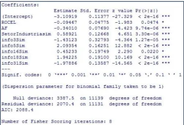
Given this, estimation was started again in the way described before. First, all variables were included but info31, and step by step, eliminating the variables with highest p-value, the best model in terms of residual deviance was reached. Again, and disregarding TVV variable because of the warning message already described, another best model was reached. This last model is going to be referred to as Model 1, while the best model including TVV as Model 2.

Figure 1 – R software output for the estimation of Model 1

Figure 2 – R software output for the estimation of Model 2

11





2

11131



. When comparing both models, given that they are nested models, Model 2 is preferable in terms of residual deviance, as expected. This is because the increase by one degree of freedom from Model 2 to Model 1 is not worth, since the increase in

deviance is greater than 3.841, the 95th percentile of 2

 

1



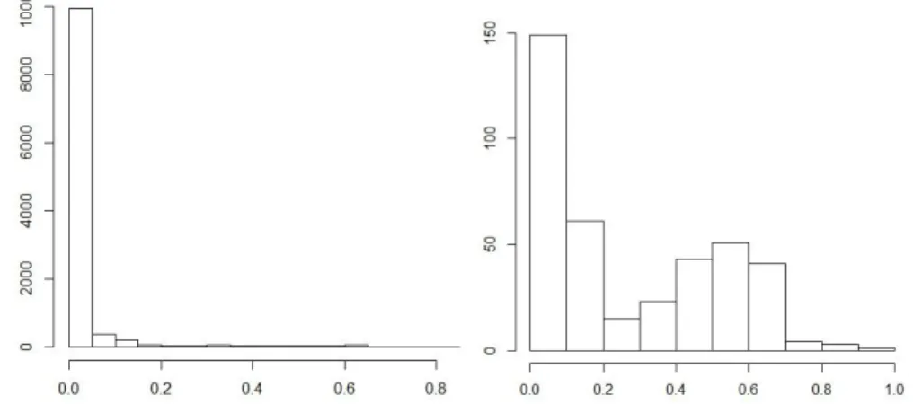
. With an illustrative purpose, Figure 3 shows the probabilities of default estimated by Model 1.

Figure 3 – Fitted probabilities of default for obligors not in default (left) and in default (right) for 2014 according to Model 1

In terms of the fitted probabilities, we can see that the great majority of obligors not in default have a probability of default close to 0. This is not verified for the ones in default. Actually the dispersion of the probability of default is not centred on 0. However, for a considerable number of obligors in default, the estimated probability of default is close to 0, which might show the weaknesses of the model already discussed. Economic conjuncture might also be an important point, since default might have occurred in cases where it was not expected at all.

The prediction power of a model is usually quantified through the Receiving Operator Characteristic (ROC) curve and the area under it. The ROC curve corresponds to the plot of the true positive rate against the false positive rate, for each threshold for considering that default is predicted. These rates are estimated, in our case, as the percentage of obligors for which default was predicted and actually happened and the percentage of obligors for which default was predicted and did not happen, respectively. The closer the area under this curve is to one, the better the model is.

12

2015, the prediction power of these two models can be calculated. Using the package ROCR of the software R, the ROC curves for both models are shown in Annex F. In terms of predictability, we can conclude that both Model 1 and Model 2 show a good explanatory power, given the area under the curve of 0.9139 and 0.9140, respectively.

Given all similarities between models, we are going to consider only Model 1 in the application of what follows.

3. AGGREGATE LOSS

A proper risk management of an insurance policy portfolio asks for the monitoring of its risks. These risks are quantified in the future, when the company is liable to pay the claim amount. However, it is of interest to predict today the total loss that may arise from the portfolio in the future.

Risk Theory is a branch of actuarial mathematics that aims to describe technical aspects of the insurance business through mathematical models. It might have its roots when a portfolio was first thought as a sum of insurance policies. Considering this, the aggregate loss from the portfolio is the sum of the losses arising from each individual policy.

Let S be the aggregate loss random variable of a portfolio of

n

independent policies in

a given period of time. Therefore, if

X

_i is the random variable for the loss arising from

policy i, then

1 n

i i

S X







where

 

X

_i are independent random variables, not necessarily identically distributed.

This is actually known as the individual risk model. Under this model, we consider that

each

X

_i has a mass point at 0, as it is not expected that all policies result in a claim.

Another way of modelling the random variable S is considering claims as arising from

13

variable, then the aggregate loss random variable is modelled as

0 N

i i

S X







with X₀ 0.

For it to be possible to deduct some interesting results, it is usually assumed that the

random variables

 

X

_i are independent and identically distributed, and independent of

N

, where Xi denotes the severity of the th

i

claim in the portfolio in the period of time

under consideration. Under these assumptions, this model is known as the collective risk model.

As a matter of fact, the choice of the risk model depends on the framework of the problem under study. In this work, we want to model aggregate losses from a portfolio of loans of a bank. In fact, besides the fact that Risk Theory was first thought to insurance portfolios applications, it is possible to apply these models to the portfolio in question. By changing the interpretation of the variables in the model, this portfolio of loans is perfectly comparable to a portfolio in the life insurance context.

Let us consider a group life insurance portfolio that pays a fixed amount in the event of death. Interpreting policyholders as obligors, probability of death in a period of time as the probability of default and the amount that the insurance company is liable to pay in the event of death as the amount of money in default, we are in the context of the loans portfolio. In this work, and for prudent reasons, the amount of money in default is going to be considered as the amount lent at the time that the default happens.

14

Considering claim frequency, we remark that a reasonable assumption is that it is Poisson distributed. Let us consider a portfolio of

n

loans, and group obligors with

equal probability of default. Let

n

_i be the number of obligors with probability of default

i

p

. In each group, we can say that the number of defaults random variable

N

_i is binomial distributed, i.e.

N

i

Bi



n p

i

,

i



. However, for a sufficiently large portfolio and

given that

p

_i is expected to be small, the distribution of

N

_i can be approximated

by a Poisson distribution with parameter



_i  n_i p_i. It is worth noting that this

approximation of a binomial to a Poisson random variable preserves its expected

value. Another possible approximation would be by matching the value of

the probability at zero, i.e.

Pr



N

i



0



, which results in a Poisson parameter





ln 1

i

n

i

p

i



 



. At portfolio level, as the sum of independent Poisson random variables is still Poisson distributed, these approaches result respectively in

i i

i

n p







and _i

ln 1



_i



i

n

p



 





, where



is the parameter of the claim frequency

random variable

N

.

For small values of p_i, these two approaches are expected to give similar results.

However, in our recent economic situation, this was not the case for many obligors. Therefore, both approaches will be considered further up, being referred to as Approach A and Approach B, respectively.

In terms of claim severity, when an obligor defaults, the amount of default is fixed and equal to the amount of the loan. This means that the claim severity random variable is

a multiple of a binomial random variable. Particularly, if

L

_i is the amount of the loan of

obligor i, then the claim severity random variable equals

L N

_{i i}. In this context, it is worth considering the following theorem and its corollary.

THEOREM 1: Suppose that

S

_j has a compound Poisson distribution with Poisson

parameter



_j and severity distribution with distribution function

 

j

X

F x , for

1, 2, ...,

15

compound Poisson with Poisson parameter

  

   

_{1 2}

...



_n and severity

distribution function

 

 

1 j

n j

X X

j

F x



F x









COROLLARY 1: Let

x x

₁

,

₂

, ...,

x

_n be different numbers and suppose that

N N

₁

,

₂

, ...,

N

_n

are independent random variables, each of them Poisson distributed with parameter

i



. Then, the random variable

S



x N

_{1 1}



x N

_{2 2}

 

...

x N

_{n n} is compound Poisson with 1 2

...

n

  

   



and claim severity probability density function

 

, if , 1, 2,...,

0 , otherwise

i

i X

x x i n f x





 _{ }

   

Given this corollary, we can conclude that the aggregate loss random variable S of our

portfolio of loans can be approximated by a compound Poisson random variable. In fact, if we divide our portfolio into groups of obligors with the same characteristics, i.e.

same probability of default

p

_i and same amount of loan

L

j, then we have

j ij i j

S





L N

where N_ij Po

 



_ij , with



_ij



n p

_{ij i} or



_ij

 

n

_ij

ln 1





p

_i



, is the claim frequency random variable of the group of the

n

ij obligors with probability of default

p

i and

amount of loan

L

_j. The collective risk model consists in considering the claim

frequency random variable

N

to be Poisson distributed with parameter



and, when a

default occurs, it can take values L_j for

j



1, 2, ...

with probability equal to ij

i ij j i









16

portfolio into groups with the same probability of default and same amount of the loan would result in one obligor per group. This fails to verify that the parameter n_ij is large

enough. We are going to ground this assumption on Credit Suisse Financial Products (1997, p. 35), where it is referred that besides the fact that the probabilities of default are all different, the approximation of the claim frequency random variable to a Poisson random variable is a good approximation. On the other hand, by comparing the probability generating function of the aggregate loss under the individual risk model context with the probability generating function of an approximation by the corresponding compound Poisson distribution, Gerber (1990, p. 97) points out that the smaller the probabilities of default are, the better the compound Poisson approximation is. In our particular case, even with relatively large fitted probabilities of default, given that the variance of the Poisson random variable is higher than the Binomial one, this assumption will actually be applied since it is a prudent one.

The next step after defining the aggregate loss random variable is to find its distribution

function, which depends upon the distribution of the random variables

N

and

 

X

i . It

is possible to find its exact distribution function by convoluting the distribution functions

of

 

X

_i . However, when considering practical applications on relatively large portfolios,

this method is time consuming in terms of calculations. To overcome this, iterative methods involving fewer amounts of computations were developed to approximate the distribution function of the aggregate loss random variable.

3.1. Panjer's recursion formula

Let us consider the set of discrete random variables X that satisfy the following

formula, being

p

n



Pr



X



n



and a b,  ,

1

,

1, 2, ...

n n

b

p

a

p

n

n









_



_







This set of random variables is known as ( , , 0)a b family and to it belong distributions

17

that it belongs to the



a b

, , 0



family with a0 and b



, since





1

1

! 1 !

n n

n n

e e

p p

n n n n



_

_



_

_

  



  



Panjer’s recursion method is an iterative method to find aggregate loss probability density function in the context of the collective risk model. For an aggregate loss

random variable such that the claim frequency distribution belongs to the



a b

, , 0



family, let g the aggregate loss density function and f the claim severity density

function, taking only values on the non-negative integers. _{Panjer’s recursive formula is}





1

1

( )

( ) (

)

,

1, 2, ...

1

(0)

(0)

(0)

x j N

j

g x

a b

f j g x

j

x

af

x

g

P

f





_



_



_

_







_

_

_





_





where P_N is the probability generating function of

N

.

If we consider the aggregate loss to be compound Poisson distributed, Panjer’s

recursive method is

1 (0)

1

(0)

( )

( ) (

)

f x j

g

e

g x

j f j g x

j

x





  



_















3.2. Discretization of the claim frequency random variable

Considering the application of Panjer’s recursion method in a practical environment, one should be aware of the frequent need for a discretization of the claim severity distribution. In fact, beyond this need, it is actually needed to transform claim severity distribution into an arithmetic distribution. An arithmetic distribution is meant to be a discrete distribution function such that all points at which a step happens are multiples of some positive number.

18

monetary unit of 1500 is defined, a loan of then 7500 is now considered as a loan of 5. However, it might be the case that there is a loan of 14000, which corresponds to a loan amount of 9.33 in the unit set.

There are sundry methods to “arithmitize” the claim severity distribution. The simplest

ones are methods of rounding, either up, down or to the nearest. According to these methodologies, and considering the previous example, a loan of 9.33 would be considered as a loan of 10 in the first method and a loan of 9 in the last two methods.

In terms of probability density function, the value

f



9.33



is now accounted as

f



 

10

or

f



 

9

, respectively. Gerber (1990, p. 94) describes a forth method, which he calls

Rounding and which consists of a rounding method to the nearest that keeps the expected value of the distribution, after an adjustment to the individual probability of default.

Another possible method, which is the one to be considered in this work, is called the method that matches the mean of the distribution. Again, and as the name suggests, after the transformation of the claim severity random variable X into an arithmetic

random variable

X

, the expected value of the distribution is maintained. Formally, for

a monetary unit h, the density function

f

 of

X

 is defined recursively as

 

1 0 1

: ... j

j j _j X

f f f  f 



 F hy dy

In practical terms and because in our particular case

F

_X is a step function, instead of

allocating

f



9.33



into

f



 

10

or

f



 

9

as in the methods of rounding, the method

that matches the means implies that

f



9.33



is proportionally split contributing to both

 

10

f

 and

f



 

9

. Gerber (1990, p.95) calls this method Dispersion and describes it

in the context of discrete random variables, where this conclusion is clearly seen. In the

context of the example given, we would have that

f



9.33



would contribute





10 9.33

9.33

10 9

f





to

f

 

9

 _and

9.33 9





9.33

10 9

f





to

f

 

10

 _.

19

the portfolio have the same upper or lower bound in terms of the chosen monetary unit. For instance, if we would have also a loan of 16000 in our example, which corresponds to 10.67 in the monetary unit set, then besides the contributions already described,

 

10

f

 would have to have reflected a contribution of

10.67 10



10.67



11 10

f





from this

loan.

In the case of our database, the exposure amount of the loans ranges widely. Due to confidentiality reasons, the amount of the loans will not be shown and therefore the choice of the monetary unit will not be discussed. After expressing all loan amounts in the monetary unit, the highest loan is of 80 000. It was not considered a higher monetary unit, and thus a less thin _“arithmatization_”, because nearly 56% of the obligors have loans whose amounts are below 50 in the chosen monetary unit.

All in all, after approximating the claim severity distribution accordingly to Corollary 1, it is discretized applying the methodology discussed in this section.

3.3. Results

In this section we are going first to discuss the fitted values for the year of 2014, comparing them to the actual experience. Then, we are going to project the default for the year of 2015.

As already said, for the year of 2014, 391 defaults were registered. According to Approach A, the fitted probabilities sum up 391. This is obviously an expected figure, as the expected number of the Poisson distribution



is the sum of individual probabilities according to this approach.

For

N

Po(391)

, we have that





391 170

Pr N 0 e 1.55 10  . However, taking into

account the fitted probabilities p_i, the probability of no default in the portfolio actually

equals





210

1

_i

1.43 10

i

p











. Therefore, it is expected that the Poisson parameter

20

Applying Panjer’s algorithm for the year of 2014, the aggregate loss distribution function is estimated. Thus, the percentile of the curve at which the registered loss is can be found. In this year, a total amount of 2 469 693 was lent, in the chosen monetary unit, being the total amount in default equal to 117 700. According to the adopted definition of loss, the actual loss equals 117 700, 4.77% of total loan amount. Given this percentage, the estimated percentile is a curious result.

Table III

Percentile of the loss that actually occurred in 2014

At first these figures seem not to be reasonable. Actually, this emphasizes the questions already pointed out regarding the validity of the model. Besides this, there are three important facts that support why these figures were obtained with this model. First, the majority of the loans in our portfolio are small loans (after expressing its value in the monetary unit): as already pointed out, 56% of the loans are below 50. Second, the estimated probability of defaults for loans greater than 10% of 117 700, which are only 23 loans, are considerably small, having a mean default rate of 1.83%. Therefore, the model for the estimation of the probability of default is limited in predicting default from obligors with the largest loans, which are the ones where principal focus should be. Finally, and concerning the values of the loans that actually defaulted, 385 loans were between 0 and 2000, 4 loans between 2000 and 6000 and 2 loans between 24 000 and 26 000. In fact, the two largest defaulted loans are amongst the largest 12 of the portfolio, which is the reason for the large percentile of the registered loss.

Regarding the year of 2015, the one we are interested in projecting, the following table shows the Poisson parameter, which actually is the expected number of defaults, under Approach A (Po_A) and Approach B (Po_B).

Table IV

Poisson parameter for year of 2015

Concerning the aggregate loss distribution, R software was used, particularly its

Po_A 0.9497 Po_B 0.9114

Model Percentile of 117 700

Model Poisson parameter

Po_A 384.70

21

package actuar, which includes Panjer’s algorithm. Given the considerable large values

for



_{, Panjer’s approximation may be questioned} about its validity, as its starting value is a very small value. The function aggregateDist of the referred package of R draws

attention to this problem, saying that Panjer’s algorithm might not start or end if the

value of



is too large. The truth is that no error or warning was returned, maybe because our values for



do not reach the too large threshold.

In this section and subsequent, the analysis of the estimated aggregate loss distribution will be made considering five percentiles in the tail of the distribution. Besides this, the estimated probability density functions for both models are shown in Annex G. In terms of percentile amounts, results are presented in Table V.

Table V

Tail percentiles of the compound Poisson aggregate loss for the year of 2015

4. CREDITRISK

+

There are four credit risk models that are recurrently considered as the most relevant ones: CreditMetrics, KMV PortfolioManager, CreditPortfolioView and CreditRisk+_.

Briefly describing them, CreditMetrics and KMV Portfolio Manager are usually classified as market value models. In the case of CreditMetrics, risk groups are defined accordingly, for instance, to credit quality classification of the company, being the worst risk group related to default. The probability of default is therefore equal to all obligors in the same risk group. Then, and based on historical record, the probability of moving from one state to another is estimated, entering in the credit migration framework. Using Monte Carlo simulation, portfolio default loss distribution is then generated according to the market value change of the asset portfolio of the company due to credit migration only. Market value change is tracked consistently with Merton’s Model, an option pricing model for the valuation of equity based on Black-Scholes, extending it to incorporate credit migration.

90 95 97.5 99 99.5

Po_A 96 018 112 194 131 101 149 531 161 686 Po_B 120 154 136 323 153 942 173 136 185 783

22

Concerning KMV PortfolioManager, the approach is to derive individual probabilities of default, the Expected Default Frequency (EDF), of each obligor rather than historical transition frequency. Following Merton_’s Model too, _{the term “distance to default” is} defined. An extension to Merton’s Model is also done, to account for the refinancing

abilities of companies. _{EDF is defined as a function of the “distance to default”, which} depends on the firm’s financial structure. Based on the estimation of the correlation between default probabilities and default record, credit rating migration matrix can be derived as well as default loss distribution.

CreditPortfolioView is classified as the econometric model, as the probability of default is defined to depend on macroeconomic scenarios. By setting up a multi-factor model to account for systemic risk, probability of default is estimated through a logit model. According to this model, default loss distribution is derived taking into account the relationship between credit migration matrix and macroeconomic indicators.

Among credit risk models, CreditRisk+ _{is classified as the actuarial model. It is going to}

be studied and described in detail in the next two subsections. In the first one, we are going to compare the simplest form of this model to the work developed in Section 3. Then, it is going to be briefly shown how to reach CreditRisk+ _{formula in its generalized}

form and put it into practice in our database.

By the end of Section 4, it should be clear the reason why CreditRisk+ _{is considered to}

be the actuarial model.

4.1. CreditRisk+ with fixed default rate

CreditRisk+ _{model does not include a methodology for the estimation of the}

probabilities of default. Nevertheless, this is required as an input to the model.

23

Concerning the arithmatization of the default severity random variable, exposure is adjusted by some unit amount. Then, and to preserve the expected loss, a rounding adjustment is made to the expected number of defaults. This is actually the referred Rounding method described by Gerber (1990, p. 94).

The next step is to find the probability generating function of the aggregate loss arising from the portfolio. Without referring to the theoretical background, CSFP (1997) concludes that the probability generating function of the aggregate loss random variable is of the form of a compound Poisson random variable, besides that they do not classify it as a compound Poisson explicitly. Actually, the probability generating function of the claim severity is consistent with Corollary 1.

Finally, an iterative algorithm to find the density function of the aggregate loss is deduced. In their notation, the algorithm is presented as

:

j j

j

n n

j n

A

A

n







 





where A_n is the probability that an aggregate loss of amount n occurs and



_j and



_j

are respectively the exposure amount and the expected loss in exposure band

j

,

expressed in the settled monetary unit. The relation between these two quantities is

j j j



 

 

where



_j is the expected number of defaults in exposure band

j

.

In our notation,



_j is



_j and



_j is simply

j

. Therefore, the algorithm presented in

CSFP (1997) in our notation is

1 1

( ) ( ) ( )

n n

j j

j j

j

g n g n j j g n j

n n



_





 





 





This is in fact _Panjer’s recursive formula since, according to the Corollary 1,

( ) j

f j







Concluding, as it is now perfectly clear, the simplest form of CreditRisk+ is a direct

24

4.2. CreditRisk+ with variable default rate

CreditRisk+ _{model generalizes the simpler model discussed in the previous section.}

After introducing volatility to the probability of default and sector analysis, a new iterative formula is deduced following the same reasoning.

The concept of sector is user adaptable. A sector might be interpreted as the sector of activity, the size of the company or even the country of domicile of the obligor. The idea is to make a partition in the set of obligors in such a way that the probability of default of the obligors in a specific sector is influenced by the same external uncontrollable factors. As in CSFP (1997), we are going to assume that each sector is driven by only one factor.

The underlying factor of each sector will influence it through the total expected rate of defaults. Therefore, the total number of defaults arising in sector k is going to be a

random variable N_k with mean



_k and standard deviation



_k.

Formally, instead of having N_k Po

 



_k , where



k is the expected number of losses

in sector k, which corresponds to the sum of individual probabilities of default of obligors in that sector, we are now going to assume that N_k given  k



k follows a

Poisson distribution with Poisson parameter

 

_{k k}. Therefore, _k is a random variable that accounts for the volatility in the individual probability of default. The key assumption of CreditRisk+ _{is that}

k

 follows a Gamma distribution. For the parameterization of the Gamma distribution, we are going to follow the one also used by Klugman et al. (2004).

To find the parameters of this distribution, we are going to impose that the expected value of _k is 1, so that the expected the number of claims in sector k is



_k. Hence,

being 2 k



the variance of k Gamma



 

k, k



, we have that

2 2

1

Gamma

,

k k

k











_

_

25 We can easily deduct that

 

 



_

_





_

_



2

1

1 2

1 1 1

k k

k k _k

k k

z

N N

N k k k k

P z E z E E z E e  M



z

 

z            _{ } _{ }  _ _{ }     where k

M_ is the moment generating function of _k. This last expression is the

probability generating function of a Negative Binomial random variable with parameters

2

1 _k

r



and 2

k k

  

 , in the Klugman et al. (2004) parameterization. We can

therefore conclude that N_k follows a Negative Binomial distribution.

After finding the distribution of the claim frequency, we are interested in finding the aggregate loss distribution within each sector. Let us find its probability generating function. For simplicity reasons, the subscript k is going to be dropped in the following

proof, but it must be kept in mind that we are within the sector. Hence, in the context of mixed frequency models, it is known that

 

   

S S

P z 



P_ z f_

 



where P_S is the probability generating function of

S

and f_ the probability density

function of



. It is important to remark that S  



is the aggregate loss random

variables for the fixed default rate case. Knowing

 



, S  



is a compound

Poisson random variable with probability generating function

 

P_X z 1

S

P

_

z



e

 

where

P

_X

 

z

is the probability generating function of the claim severity random variable

with density function accordingly to Corollary 1, eventually after arithmatization. Hence, we have that

 

   

 

 





 

 

 

   











 



 

 

 

 

   







 



 





2 ₂ 2 2 2 2 2 2 2 2 2 1 1 1 1 2 2 1 1 1 1 2 1 2 1

2 1 1 1 1

1 1

2 _{2 2}

1

1

1

1 1

1 1 1

X X X w _w P z S _w

w P z w

w

w

w P z w

X

w w

X

e P z e

w w

e

w w

w P z _e

w _{w P z w}