II E UNICEA LEXANDRAM ADEIRAB ALAU

(1)

M

ASTER IN

A

CTUARIAL

S

CIENCE

M

ASTERS

F

INAL

W

ORK

DISSERTATION

P

_{REMIUMS AND}

R

_{ESERVES IN}

L

_IFE

I

_NSURANCE

P

_OLICIES:

T

_HE

W

_ORST-CASE

S

_{CENARIO AND}

S

_OLVENCY

II

EUNICE

ALEXANDRA

MADEIRA

BALAU

(2)

M

ASTER IN

A

CTUARIAL

S

CIENCE

M

ASTERS

F

INAL

W

ORK

DISSERTATION

P

_{REMIUMS AND}

R

_{ESERVES IN}

L

_IFE

I

_NSURANCE

P

_OLICIES:

T

_HE

W

_ORST-CASE

S

_{CENARIO AND}

S

_OLVENCY

II

EUNICE

ALEXANDRA

MADEIRA

BALAU

SUPERVISOR:

PROF.

ONOFRE

ALVES

SIMÕES

(3)

Acknowledgements

First of all, I would like to thank my advisor, Professor Onofre Simões, for his entire availability and care for my work. His suggestions and relevant observations, as well as the constant support and motivation were indispensable to the development of this thesis.

Special thanks go to my Family, particularly to my parents and my brother who often had to deal with my bad temperament and exhaustion, for their unconditional support.

To Filipe for all the patience during the last few months.

(4)

Resumo

As reservas de capital representam um instrumento fundamental no processo de gestão de risco das empresas de seguros, sendo utilizadas no cálculo do capital económico e re-gulamentar. Como o valor das reservas e dos prémios é fortemente influenciado pelos pressupostos atuariais utilizados, a escolha adequada das bases técnicas é um dos temas de principal interesse para as Companhias de Seguros e para as Entidades Reguladoras.

O principal objetivo deste trabalho é o estudo de um método de construção de cenários biométricos para o cálculo de reservas e prémios, adotando uma posição conservadora em relação às bases técnicas de segunda ordem, seguindo a orientação de dois trabalhos fundamentais neste domínio, Christiansen (2010) e Milbrodt and Stracke (1997). Este cenário é determinado através da resolução de um problema de maximização da reserva prospetiva que nos permite definir as bases biométricas de primeira ordem que representam o pior caso do ponto de vista do Segurador. As apólices do ramo vida são descritas pelo modelo Markoviano de estados múltiplos, sendo as reservas prospetivas calculadas recorrendo à equação de Thiele.

O novo regime de solvência da União Europeia, Solvência II, também recorre à noção de piores cenários, por forma a quantificar os requisitos de capitais no ramo vida, em-bora com uma definição diferente. Assim, um objetivo adicional, e também importante, deste trabalho é procurar integrar o método estudado no enquadramento estabelecido pelo projeto Solvência II.

O novo método, bem como as propostas anteriores existentes na literatura, serão ob-jeto de apresentação e discussão, recorrendo nomeadamente a dois Casos de Estudo, que permitirão observar a sua praticabilidade no cálculo dos prémios e das reservas, enquanto se avalia uma possível aplicação no enquadramento estabelecido em Solvência II. Por forma a fazê-lo, os casos analisados pelo autor serão estendidos a outros produtos que, embora não sendo comuns no mercado Português, pela sua complexidade, nos permitem mostrar toda a versatilidade inerente ao modelo e tirar importantes conclusões.

(5)

Abstract

Reserves are a fundamental tool in insurance risk management since they are used to determine the economic or regulatory capital required for insurers to remain solvent. As the values of reserves and premiums are strongly dependent on the actuarial assumptions used, the choice of the adequate elements of the technical basis is a major concern of both regulators and insurance companies.

The main purpose of this work is to study a method for the construction of biometric worst-case scenarios that allow premiums and reserves to be on the safe side with respect to given confidence bands for the biometric second-order basis, following the essential works of Christiansen (2010) and Milbrodt and Stracke (1997). This scenario is obtained by solving a maximization problem for the prospective reserve that allows one to find the worst-case biometric valuation basis from the insurer’s point of view. In life insurance, policies are often described by the multi-state Markov model of life contingencies and the prospective reserves computed using Thiele’s equation.

The new solvency regime of the European Union, Solvency II, also uses worst-case scenarios, although constructed in a different way, in order to quantify the solvency capital requirements for life insurance business. Thus, a further important purpose of this thesis is to integrate the method in study under the Solvency II framework.

The new method, as well as the previous approaches offered in the literature, will be presented and discussed with two Case Studies, demonstrating the usefulness for the calculations of premiums and reserves, while a possible application in the calculation of solvency reserves in Solvency II are introducing. In order to do so, the examples discussed by the author are extended to products, which although not common in the Portuguese market, are complex situations that allow us to show the versatility of the model in study and to derive significant conclusions.

(6)

List of Figures

4.1 Disability Income Protection & Critical Illness Model . . . 30

A.1 Overall structure of the Solvency Capital Requirement. Source: EIOPA (2014b) . . . 41

A.2 Log mortality rates: BE, GFK95 and GKM80 . . . 42

A.3 Log mortality rates: GFK95 & GKM80; DAV2004R & DAV2008T . . . 42

A.4 Log mortality rates: BE of GFK95 & GKM80; BE of DAV2004R & DAV2008T . . . 43

A.5 Log disability rates: BE, TPD and SwissRe2001 . . . 43

A.6 Term Structure of Interest Rates - 31 December 2013 . . . 44

A.7 CS 1.5 - Prospective reserveVa(t) . . . 47

A.8 Log transition intensities . . . 48

A.9 CS 2 - Prospective reserveVa(t) . . . 50

(9)

List of Tables

4.1 CS 1.1 and CS 1.2 - Premiums and technical interest rates . . . 26

4.2 CS 1.1 and CS 1.2 - Prospective reserveVa 0− . . . 26

4.3 CS 1.3, 1.4 and 1.5 - Premiums and technical interest rates . . . 28

4.4 CS 1.3, 1.4 and 1.5 - Prospective reserveVa 0− . . . 28

4.5 CS 1.5 - Standard formula of Solvency II . . . 29

4.6 CS 2 - Prospective reserveVa 0− . . . 31

4.7 CS 2 - Standard formula of Solvency II. . . 32

4.8 CS 2 Sensitivity analysis - Prospective reserveVa 0− . . . 33

A.1 Correlation matrix for biometric life insurance risks. Source: EIOPA (2014b) . . . 41

A.2 CS 1 - Internal stress scenarios and Solvency II stress scenarios . . . 45

A.3 CS 1.1 and CS 1.2 - Standard formula of Solvency II . . . 46

A.4 CS 1.3 and CS 1.4 - Standard formula of Solvency II. . . 46

A.5 CS 2 - Internal stress scenarios and Solvency II stress scenarios . . . 49

(10)

There is nothing more practical than a good theory.

(11)

Chapter 1

Introduction

Since the early 18th century that actuaries applied scientific principles and techniques to life insurance problems involving risk, uncertainty and finance. Although the basic risks insured have not changed, contracts have become more complex in recent years as well as the techniques needed to manage them.

The insurer should use those techniques to maintain the total liabilities plus the com-pany’s net value equal to its total assets. Assets are mainly investments such as bonds, equities and property, resulting from the collection of premiums from the policyholders and from earnings on the investments. On the other hand, the liabilities of life insurers primar-ily comprise the reserves hold to back its obligations to policyholders and beneficiaries. As a matter of fact, the calculation of the sum of the reserves for all policies in force and the value of all the company’s investments, at the valuation time, is an important element in the financial control of an insurance company.

The legal framework for the insurance activity in member states of the European Union (EU) is based upon common rules. In Portugal, the Portuguese Insurance and Pension Funds Supervisory Authority (ISP) ensures that insurance companies carry out their busi-ness in accordance with the European law, supervising the prudent management. In order to do so, ISP requires each company to maintain its reserves at a level that will assure payment of all policy obligations as they fall due. In fact, reserves are not only used to determine the profit or loss for the company over any time period, but also to determine the economic or regulatory capital needed to remain solvent, being a fundamental tool in insurance risk management.

(12)

probabilities, reactivation probabilities and interest rates. Following Macdonald (2004), technical bases have three main purposes: pricing, i.e. setting premiums, valuation for solvency and valuation in order to measure and distribute surplus. In many countries, the basis used to calculate premiums, called premium basis, differ from the assumptions used to calculate the reserves, that is, the valuation basis. Another distinction is between first-order basis and second-order basis. While first-order basis include a safety margin, making conservative or safe-side assumptions about the future, the second-order basis, in principle, do not contain any margin and consists in the best estimate with respect to the insured population, being often called experience basis.

The past has shown that the variation in the actuarial assumptions can be wide within a contract period, for instance, the recent increase in life expectancies in many developed countries. The influence such changes can have on premiums and reserves is an important issue and the choice of the technical basis is a major concern of regulators and insurance companies. As a matter of fact, premiums and reserves should be set on the safe-side, in the sense that they should be high enough to cover the benefits in all possible scenarios. In order to do so, it is a common method to choose first-order technical basis that represents some worst-case scenario for the insurer.

Literature offers three ways for the construction of these scenarios. There is a first method based on the sum-at-risk which was developed by Lidstone (1905), Norberg (1985), Hoem (1988), Ramlau-Hansen (1988) and Linnemann (1993). Verbally, it studies the fin-ancial effect at any point in time resulting from the transition of the policyholder from one state to another. The authors showed that, for a given first-order basis with corresponding sums-at-risk for the different states of the policy, the premiums and reserves are on the safe side if: the second-order basis is smaller than the first-order basis when the first-order sums-at-risk are positive; or the second-order basis is greater than the first-order basis when the first-order sums-at-risk are negative.

The two other methods are based on derivatives. The second one was presented by Dienst (1995), Bowers et al. (1997), Christiansen and Helwich (2008) and Christiansen (2008a,b) and approximates the relevant functions with local linearisations by using first-order derivatives, given that worst-case scenarios can be found much more easily for linear mappings. The third one, developed by Kalashnikov and Norberg (2003), differentiates the reserve and premium with respect to one arbitrary real parameter and, using the assumption of normality, obtains confidence bands for them in an one step-approach.

However, as we will see later, none of these three methods is an exact method and all of them have problems: the first method does not tell us how to find the first-order basis; the second method works only for narrow confidence bands and yields only approximate results; the third method runs counter to the traditional rules of insurance regulation in many countries. Trying to fill this gap in the literature, Christiansen (2010) presents a new method.

(13)

premi-ums and reserves be always on the safe side with respect to given confidence bands for the biometric second-order basis. Thus, one should choose the first-order valuation basis that maximizes the reserve with respect to all biometric scenarios within the bounds imposed for our actuarial assumptions. The method allows to construct such scenarios for homo-geneous portfolios of single life insurance policies and the results are especially interesting for life insurance policies with a mixed character, i.e., survival and occurrence character.

There are two main purposes in this thesis:

1. To explore the method introduced by Christiansen (2010) and adapting it to the Portuguese case (at this point, use was made of the practical knowledge the author acquired while performing her professional tasks);

2. Attention should be paid to the fact that the new solvency regime of the EU, Solvency II (Directive 2009/138/EC), uses worst-case scenarios for the calculation of the solvency capital requirement (SCR) in life insurance business. Thus, a pos-sible application of this method in the Solvency II framework is also discussed.

(14)

Chapter 2

Life Insurance

The origins of the concept of life insurance go back to burial clubs in Rome, in 100 B.C., which were created to pay for the funeral of members. Norton (1852) refers that traditional life insurance were established in the early 18th century, in order to provide financial assistance to widows in the event of policyholder death. These policies remains very similar to the contracts written up to the 1980s, experienced enormous changes in the last three decades.

2.1 Types of contracts

In its simplest form, an insurance policy is a contract between two parties placing obliga-tions on both of them. The policyholder agrees to pay an amount or a series of amounts to the insurer, called premiums, in return for a later payment or set of payments from the insurer, called benefit(s), if and when the event insured against occurs.

Life insurance policies exist in many forms, most of them providing considerable flexib-ility in premiums (amount, duration and frequency) and benefits (amount and the circum-stances under which these will be paid). The benefits payable under simple life insurance contracts are of two main types: insurance or annuity. While the term insurance is usually used when the benefit is paid as a single lump sum, contingent on the death or on survival of the policyholder to a predetermined maturity date, an annuity is a benefit in the form of a regular series of payments, usually depends on the survival of the policyholder.

(15)

pays a sum assured either on death of the policyholder or at the end of a specified term, whichever occurs first.

Annuity contracts provides payments of amounts, which might be level or variable, at stated times, provided a life is still alive. There are many variants of annuity contracts, described e.g. in Garcia and Simões (2010). For instance, a whole life annuity provides payments until the death of the annuitant; if the payments are made for some maximum period, provided the annuitant survives that period, it is called a term annuity; and in the deferred annuity the start of payment is deferred for a given term.

There are other life contingent risks, depending on the state of health of the policy-holder, described e.g. in Booth et al. (2005) as health insurance products: income pro-tection insurance; critical illness insurance; long-term care insurance and private medical insurance. For instance, while an income protection insurance replaces some income to the insured whilst they are unable to work, by reason of illness or injury, a critical illness insurance pays a benefit on diagnosis of a severe condition, such as certain cancers or heart disease.

In recent years, in order to competing for policyholders’ savings with other institutions, insurers have provided more flexible products that combine the death benefit coverage with a significant investment element, known as the modern insurance contracts (Dickson et al., 2012).

2.2 The loss random variable

The cash flows for a life insurance contract consist of the insurance and/or annuity benefit outgo (with associated expenses) and the premium income. All of the cash flows in a contract are uncertain, depending on the death, survival or possibly the state of health of a life, unless the contract is purchased by a single premium, in which case there is no uncertainty regarding the premium income. Therefore, the loss incurred by the insurer on a particular policy can be modelled with the loss random variableL.

Definition 2.2.1. Consider a policy which is still in forcetyears after it was issued. The

random loss variable at timet,L(t), is the difference between the present values of future

outgo and of future income: L(t) =P V [F uture Outgo]−P V [F uture Income].

Insurers wish to determine a distribution for L(t) with the purpose of finding the adequate premium for a given benefit and compute reserves.

2.3 Premiums

(16)

- one single payment, known as a single premium;

- a regular series of m payments of a constant or varying amount, made every 1/m years, typically quarterly or monthly, known as regular premiums.

The key feature of any life insurance policy is that premiums are payable in advance, so the first payment is always due at the time the policy is effected.

The benchmark principle for calculating premiums is the equivalence principle (Gerber, 1997). This method consists in finding the premiums that set the expected present value of the income equal to the expected present value of the outgo:

EP V of benef it outgo=EP V of premium income

or equivalentlyE[L(t)] = 0.

However, there are other classical methods of calculating premiums, such as the port-folio percentile premium principle or the utility principle (Bowers et al., 1997), and more contemporary approaches, used commonly for non-traditional policies, that consists in con-sider the cash flows from the contract and to set the premium to satisfy a specified profit criterion (Dickson et al., 2012; Booth et al., 2005)

2.4 Provisions and Policy Values

A reserve is the amount set aside by the insurer to meet its future obligations, i.e. to pay policyholder’s benefits and, where appropriate, future expenses. In reserve calculations it is possible to look to the future cash-flows forward leading to the calculation of present values, or backward leading to the calculation of accumulations (The Actuarial Profession, 2013, CT5 Contingencies). This concepts lead to two types of reserves:

- Retrospective reserve is the accumulated value of premiums received less benefits paid up to time t, on a specified basis.

- Prospective reserve is the expected present value of the loss random variable, on a specified basis.

The prospective reserve is an important element in the financial control because if the insurer holds funds equal to the reserve and the future experience follows the reserve basis then, averaging over many policies, the combination of reserve and future premiums will be sufficient to pay the future benefits and expenses. In general terms, at a certain point in timet,

V (t) +EP V at t of f uture premiums=EP V at t of f uture benef its+expenses

whereV(t) is the the prospective reserve at timet(Bowers et al., 1997).

(17)

2.5 Thiele’s equation

2.5.1 Reserving for a policy with discrete annual cash flows

Following Dickson et al. (2012), consider a policy issued to a life aged x under which premiums, expenses and claims can occur only at the start or end of the year. Suppose this policy has been in force for tyears, wheret≥0. Consider the(t+ 1)th year and the following notation:

- Pt: premium payable at timet;

-Et: premium-related expense payable at timet;

-bt+1: sum insured payable at time t+ 1 if the policyholder dies in the year;

-et+1: expense of paying the sum insured at timet+ 1;

-tV : prospective reserve for a policy in force at timet(t+1V denotes the prospective reserve

for a policy in force at time t+ 1);

-qx+t: probability that the policyholder, alive at time t, dies in the year;

-px+t: probability that the policyholder, alive at timet, survives to agex+t+ 1;

-Kx+t: curtate future life time for a life agedx;

-it: rate of interest assumed earned in the year. The loss random variable at timetis

Lt=

  

(1 +it)−1(bt+1+et+1)−Pt+Et if Kx+t= 0 (with probability qx+t) (1 +it)

−1

Lt+1−Pt+Et if Kx+t≥1 (with probability px+t) and therefore, the prospective reserve can be defined as

tV =E[Lt] =qx+t(1 +it)−1(bt+1+et+1) +px+t(1 +it)−1 t+1V −(Pt−Et) (2.5.1) In words, equation (2.5.1) states that the reserve at the start of the year should be equal to the present value of expected cost of the death benefits at the year end (the benefit isbt+1 plus expenses et+1 payable with probability qx+t) plus the present value of the expected cost of setting up the reserve at the year end (the reserve of amountt+1V is required with probabilitypx+t) minus the premium cash-flows (Pt−Et).

2.5.2 Thiele’s Differential Equations

The concepts presented above extend to policies where regular payments are payable con-tinuously and sums insured are payable immediately on death (Appendix A.1). In practice, it is common to represent the prospective reserve as a system of linear differential equations describing the dynamics of reserves in life insurance in continuous time. These equations are called Thiele’s differential equations and are of the form (Wolthuis, 2003; Dickson et al., 2012):

d

(18)

While the left-hand side of the formula is the rate of increase in the reserve at timet, the right-hand side explains the individual factors affecting the value of V (t). These factors are the following: interest is being earned on the current amount of the reserve and the rate of increase at timet isδ_tV ₍_t₎_{; premium income, minus premium-related expenses, is}

increasing the reserve at rate Pt−Et; claims, plus claim-related expenses, decrease this amount at rate(bt+et−V (t))µx+t.

(19)

Chapter 3

Biometric worst-case scenarios

The main reference for this work is Christiansen (2010). The model therein presented is of the most interest, since it allows one to construct biometric worst-case scenarios that let premiums and reserves be always on the safe side with respect to given confidence bands for the biometric second-order basis. In order to do so, one should choose the first-order valuation basis that represents some worst scenario from the insurer’s point of view and as such maximizes the reserve. In this chapter, we start with the theoretics of the problem, we look at the three previous approaches offered in the literature and then describe the model.

3.1 Theoretics of the Problem

Christiansen (2010) uses Thiele’s equation in the Markov model of life contingencies to derive formulas concerning the expected actual development of reserves. The author follows the general approach of Milbrodt and Stracke (1997) using the argument that it is valid to the discrete and continuous methods, as well as the mixed cases. Thus, this section is focused on these two works, essential for the development of the thesis.

3.1.1 Time-Continuous Markov Model for life and other contingencies

Multi-state models are one of the most important developments in actuarial science since they simplify and provide a sound foundation for some traditional actuarial techniques. The Markov model (Ross, 1996; Wolthuis, 2003), a special type of a multi-state model, is a very useful instrument to model life insurance and annuities as it provides sufficient generality to cover most situations in the insurance of persons and satisfy the so-called Markov property under which the future development of the process depends only on the present state and not on its full history so far.

(20)

random maps of states. At every time after policy issue the state of the policy is recor-ded and this corresponds to modelling risks by jump processes, according to the following definition (The Actuarial Profession, 2013, CT4 Models):

Definition 3.1.1. A continuous-time Markov processXt,t≥0 with a discrete, i.e. finite or countable, state spaceS is called a Markov jump process.

3.1.1.1 Time-inhomogeneous Markov jump processes

We start this sub-section by discussing the important features of time-inhomogeneous Markov jump processes and then introduce the integrated form of Kolmogorov backward Equations (used later in sub-section 3.1.2). In order to do so, consider a general insurance policy issued at time 0, with termT and modelled by a Markovian jump process(Xt)_t∈_[0_,T_]

with finite state spaceS. Transitions between states are governed by the transition prob-abilities, with the transition space denoted byJ =(j, k)∈S2_|_j₆₌_k _{. Assume that it is} an inhomogeneous time-continuous Markov process where the transition probabilities for each fixed period of time vary in time. Thus, it is necessary to specify the beginning and the end of the interval[s, t], instead of just its lengtht−s.

Definition 3.1.2. The transition probability pjk(s, t) is the conditional probability that the process is in statekat timet, given that the process is in statejat times, irrespective of the way in which state kis reached (Markov property), that is:

pjk(s, t) =P(Xt=k|Xs=j), 0≤s≤t≤T, (j, k)∈S2, P(Xs=j)>0

pjk(s, t) = 0, otherwise.

Furthermore,

pjk(s, s) =δjk, s≥0,(j, k)∈S2, (3.1.1)

whereδjk is the Kronecker delta, which is equal to 0 forj6=k and equal to 1 for j=k.

The transition probabilities satisfy properties (1)-(2) below (Milbrodt and Stracke, 1997):

(1) 0≤pjk(s, t)≤1, 0≤s≤t, (j, k)∈S2.

(2) P_k∈Spjk(s, t) = 1, 0≤s≤t, j ∈S.

In words, since the state space S is finite, there exists a finite-dimensional transition probability matrix denoted byp(s, t) = (pjk)₍_j,k₎_∈S2 where all elements are non negative

and all rows sum to unity.

Chapman-Kolmogorov equations: IfXt is a Markov process, the transition probab-ilities obey the Chapman-Kolmogorov equations:

pjk(s, t) =X

i∈S

(21)

that expresses the fact that if a process is in statejat timesand is in statekat timetthe transition occurs via some state i∈S at an arbitrary intermediate time r. Equivalently, written in matrix form we have

p(s, t) =p(s, r)p(r, t) 0≤s≤r ≤t, (j, k)∈S2.

To avoid difficulties with null-sets, the concept of regular transition matrices is now intro-duced (Milbrodt and Stracke, 1997).

Definition 3.1.3. The transition matrix p(s, t) is regular if it satisfies the Chapman-Kolmogorov Equations (3.1.2) and equation (3.1.1), without exceptional sets - null sets. If in additionpjk(s,) is right continuous for every s∈ [0, T],(j, k) ∈ S2, then p(s, t) is

called a right continuous regular transition matrix.

Intensities of transition: Intensities of transition are the fundamental concept in con-tinuous time. In order to differentiate the transition probabilities we will assume that the functionspjk(s, t) are continuously differentiable. This assumption implies the existence of the following quantities.

Definition 3.1.4. For0≤s≤t,(j, k)∈J , the transition intensity from statej to state kis

µjk(s) =

∂

∂tpjk(s, t)

t=s

= lim

h→0

pjk(s, s+h)−δjk h

and the intensity of decrement for statej is

µjj(t) =−X k6=j

µjk(t).

In addition, the matrix of transition intensitiesµjk(t) isµ(t) = (µjk)₍_j,k₎_∈S2.

Assumption 3.1.5. The intensity function for the transition from state j to state k, µjk(t), j6=k, exists.

Based on Alioum (2013), the concepts of cumulative transition intensity qjk(s, t) follow.

Definition 3.1.6. For0≤s≤t,(j, k)∈J:

(1) The cumulative transition intensity from statej to state kisqjk(s, t) = ´t

sµjk(t)dt.

(2) The cumulative intensity of decrement for statej isqjj(s, t) =−´t

sµjj(t)dt.

(3) The matrix of cumulative transition intensitiesqjk(s, t)is qJ =q(s, t) = (qjk)₍_j,k₎_∈S2.

(22)

Lemma 3.1.7. If s≥0 and (j, k)∈S2 satisfy P(Xs =j)>0, then

(1) qjk(s, r) +qjk(r, t) =qjk(s, t), s≤r≤t.

(2) limt→sqjk(s, t) =qjk(s, s) = 0.

(3) qjk(s, t)≥0 , qjj(s, t)≤0, s≤t, j6=k.

(4) qjj(s, t) =−P_k6₌_jqjk(s, t), s≤t.

(5) △qjj(t) =qjj(t)−qjj(t−)≥ −1, t >0.

(6) △qjj(t0) =qjj(t0)−qjj(t0−) =−1⇒ qjj(t) is constant on [t0, T].

Again, to avoid difficulties with null-sets, the concept of regular transition intensity matrices follows.

Definition 3.1.8. The cumulative transition intensity matrixq(s, t)is regular if it satisfies properties (1)-(6) in Lemma 3.1.7 without exceptional sets - null sets.

Assumption 3.1.9. The Markovian jump process(Xt)_t∈_[0_,T_]has a regular cumulative trans-ition intensity matrix q.

Kolmogorov backward integral equations: Define the probability of staying unin-terruptedly in the current statej in the interval [s, t] as: p_jj(s, t) = e´stµjj(r)dr_{. Let the}

residual holding time Rs be the amount of time between s and the next jump and let X_s+ =Xs+Rs. Conditional on Rs and X

+

s and using the law of total probability

pjk(s, t) =P[Xt=j|Xs=k] =δjkp_jj(s, t) +P_i6₌_j´t

spjj(s, r)µji(r)P[Xt=k|Xs=j, Rs=r−s, Xs+=i]dr

and therefore

pjk(s, t) =δjkp_jj(s, t) +X

i6=j ˆ t

s

p_jj(s, r)µji(r)pik(r, t)dr. (3.1.3)

p_jj(s, r)µji(r)pik(r, t) is the probability of remaining in state j from time s to time r, then making a transition to state i at time r, and finally going from state i to state k between times r and t. To take into account the possible values of Rs we integrate from r =sto r =t , and to take into account all possible intermediate states we sum over all possible values ofi6=j.

Milbrodt and Stracke (1997) present the backward integral equations using the cumu-lative transition intensities, as follows:

pjk(s, t) =δjk+X

i∈S ˆ t

s

(23)

3.1.1.2 Insurance benefits and premiums

Let us consider the general insurance policy introduced in 3.1.1.1. Contractual payments between the insurer and the policyholder are taken to be on a continuous time basis. At any timet∈[0, T]the policy provides (Wolthuis, 2003):

- Lump sum benefits bjk(t) upon a transition from state j to k, payable at time DT(t) ≥ t , for (j, k) ∈ J. bjk(t) are deterministic non negative functions with bounded variation and DT(t), DT : (0,∞) → (0,∞), is an increasing function introduced by Milbrodt and Stracke (1997) in order to model the difference that may occur between the payment date and the time of transition. To simplify notation, assume that DT(T) =T.

- Annuity payments Bj(t)during sojourn in a state j defined in a cumulative man-ner, i.e. Bj(t) is the total amount paid in time [0, t]. Bj(t) are right continuous deterministic functions with bounded variation. While benefits paid to the insured have a positive sign, premiums paid by the insured have a negative sign.

For reasons of simplicity, expenses and single premiums are disregarded. However, the theory may be easily developed to incorporate these topics. For instance, expenses may be considered as additional benefits.

3.1.1.3 Interest model

In the literature a large number of interest models is available (Brigo and Mercurio, 2006). Christiansen (2010), assumes that the investment portfolio of the insurance company earns interest according to the compound interest model with interest intensity function ϕand cumulative intensityΦ. In the general case, interest cumulative intensityΦcan be defined based on the interest functionr(t) as bellow (Milbrodt and Stracke, 1997).

Definition 3.1.10. Letr(t)be an interest function, non decreasing and right-continuous, equal to 1 at time zero. ThenΦ (t) =´t

0 1

r(s−)dr(s), t≥0.

It follows that the value at timesof a unit payable at time t > sis

υ(s, t) = 

Y

(s,t]

(1 +dΦ)  

−1

(3.1.5)

for partitionss < t0 < t1<... < tn=t.

Furthermore, when the cumulative intensity functionΦis a step-function, one can separate the jumps ofΦ (t) from its continuous part and get the generalized exponential formula

υ(s, t) =e(−Φc(t)−Φc(s)) Y τ∈(s,t]

(24)

where Φc₍_t_{) = Φ (}_t₎₋P

τ≤t△Φ (τ) for all t is the continuous part of Φ and △Φ (t) =

Φ (t)−Φ (t−).

Further details about (3.1.5) and (3.1.6) can be found in Jacod (1975) and Gill (1980, Lemma 3.2.1 and Appendix 4).

3.1.2 Reserves and Thiele’s Equations revisited

Naturally, the definition of prospective reserve for a policy modelled using a multi-state model continues to be the expected value of the future loss random variable, with one obvious additional requirement. Due to the Markov property, the reserve depends on the current state of the policy and the time elapsed since entering this state. Formally, considering the three basic elements of the time-continuous Markov model presented in the previous section, the Definition 3.1.11 follows.

Definition 3.1.11. The prospective reserve for the policy that is in stateiat times, given thatq is a regular matrix, is defined by

Vi(s) =X

j∈S ˆ

(s,T]

υ(s, t)pij(s, t)dBj(t)+ X

(j,k)∈J ˆ

(s,T]

υ(s, DT(t))bjk(t)pij(s, t−)dqjk(t).

(3.1.7)

Both terms in the right-hand side of the equation concern expected present values over the interval(s, T]. The first term is the expected present value of annuity payments made during the sojourn in states of the Markov chain, and the second term is the expected present value of the lump-sum insurance benefits. Random variables are both the times of transition and the states to where the transitions occur.

Under appropriate smoothness conditions, Milbrodt and Stracke (1997) show that Thiele’s differential equations are obtained differentiating (3.1.7):

d

dtVi(t) =−bi(t) + (ϕ(t)−µii(t))Vi(t)−

X

k6=i

(υ(t, DT(t))bik(t) +Vk(t))µik(t) (3.1.8)

Formula (3.1.8) can be interpreted in the same way as formula (2.5.2). During sojourns in statei, the reserve changes as a result of interest being earned at rate ϕ(t)Vi(t), and benefits being paid at rate bi(t). Transitions from state i to any other statek at time t, also lead to changes in the prospective reserve: a decrease of bik(t) as the insurer has to pay at time DT(t) any lump sum benefit contingent on jumping from state i to state k; a decrease ofVk(t) as the insurer has to set up the appropriate reserve in the new state; and an increase ofVi(t) as this amount is no longer needed (for all possible transitions we haveµii(t)Vi(t)).

(25)

cumulative transition intensity and transition intensity matrices that satisfy the backward integral equations identically, i.e.. without exceptional sets, is required.

As a matter of fact, if the cumulative transition intensity matrixq(s, t)is regular, then the transition probability matrixp(s, t) has a representation of the form

p(s, t) =Y

(s,t]

(_I+dq), (3.1.9)

whereI denotes the appropriate unit matrix. Furthermore, according to Andersen et al. (1991), the product-integral of pover intervals of the form[0, t]can be defined as

p(s, t) = lim

max|ti−ti−1|→0

Y

(_I+q(ti)−q(ti−1)),

wheres < t0 < t1< ... < tn=t is a partition of[s, t].

From this derivations, Milbrodt and Stracke (1997, Lemma 4.7) prove the regularity conditions required in the Lemma below.

Lemma 3.1.12. Let Xt be Markov, q a regular cumulative transition matrix for Xt and p defined by the product in (3.1.9). Then p is a right continuous regular transition matrix forXt that satisfies the backward integral equations (3.1.3) and (3.1.4) identically.

For Thiele’s integral equations of type 2, stronger integrability conditions, which do only make sense ifq is regular, are also required. Following Milbrodt and Stracke (1997), these are listed in Assumption (3.1.13).

Assumption 3.1.13.

(1) P_j∈S|Bj|(T)<∞.

(2) P₍j,k)∈J ´

(0,T]υ(t, DT(t))bjk(t)dqjk(t)<∞. (3)P_j∈SP₍_j,k₎_∈J´

(0,T] ´

(t,T]υ(0, s)d|Bj|(s)r(t)dqjk(t)<∞. (4)P₍_i,l₎_∈JP₍_j,k₎_∈J´

(0,T] ´

(t,T]υ(0, DT(s))bjk(s)dqjk(s)r(t)dqil(t)<∞.

At this stage, it is now possible to present Thiele’s integral equation of type 2 (Milbrodt and Stracke, 1997, Theorem 4.8).

Theorem 3.1.14. (Thiele’s integral equation of type 2) Let Xt be Markov with a regular cumulative transition intensity matrix q and p be a right continuous regular transition matrix forXt, which satisfies the backward integral equations (3.1.3) identically. Assume that the integrability conditions (1)-(4) hold and fix a version of the prospective reserve by

(3.1.7). Then for everys∈[0, T], i∈S:

Vi(s) =Bi(T)−Bi(s)− ˆ

(s,T]

Vi(t−)dΦ (t) +

X

j:j6=i ˆ

(s,T]

(26)

where Rij(t)is the so-called sum-at-risk associated with a possible transition from state i to statej at timet,

Rij(t) =υ(t, DT(t))bij(t) +Vj(t) +△Bj(t)−Vi(t)− △Bi(t),

△Bj(t) =Bj(t)−Bj(t−).

The interpretation of the system of integral equations in terms of infinitesimal sojourn payments Bi(T)−Bi(s), infinitesimal interest premiums Vi(t−)dΦ (t) and infinitesimal sums-at-risk Rij(t)dqij(t) is the same as for the classical Thiele’s equation. We should point out that Thiele’s integral equations of type 1 imply Thiele’s integral equations of type 2 and vice versa. Proofs are presented in Milbrodt and Stracke (1997).

If furtherΦand the qjk have the intensitiesϕand µjk, then (3.1.10) becomes:

Vi(s) =Bi(T)−Bi(s)− ˆ

(s,T]

Vi(t−)ϕ(t)dt+

X

j:j6=i ˆ

(s,T]

Rij(t)µij(t)dt. (3.1.11)

Additionally, from (3.1.7) we get an initial condition for Thiele’s integral equation system: Vi(T) = 0 for all i∈S.

From now on, following Christiansen’s approach (2010), the prospective reserve is defined as in (3.1.10) and (3.1.11).

3.2 The existing approaches

As already referred, before Christiansen (2010), literature offered three main frameworks for the construction of a biometric first-order valuation basis. In this section, we give a more detailed survey of these approaches.

3.2.1 Sum-at-risk

Lidstone (1905) studied the effect on reserves of variations in valuation basis and contract terms in discrete time. Lidstone’s ideas are extended to a continuous time version, using Thiele’s differential equations, by Norberg (1985). Later, Hoem (1988), Ramlau-Hansen (1988) and Linnemann (1993) studied the expected profit resulting from changes in valu-ation basis.

The basic safe-side requirement introduced for the Markov model by Hoem (1988) is

V_i∗(t)≤Vi(t),

(27)

Assuming premiums, benefits and the prospective reserve at timeT to be equal on first and second order basis, Linnemann (1993) shows that changes in the prospective reserves for a closed insurance portfolio caused by alterations in the technical basis are given by

Vi(t)−Vi∗(t) = ˆ T

t

υ∗(t, u)X

k

p∗_ik(t, u)g_k∗(u)du, (3.2.1)

whereg∗

k = (ϕ∗−ϕ)Vk(u)−Pl(µ∗kl(u)−µkl(u))Rkl(u). Observe that if g∗k ≥0 for all kand u, thenVi(t)≥V_i∗(t) for alliand tand the basic safe-side requirement is fulfilled. A sufficient condition is, of course, that ϕ∗ _≥ _ϕ _{and the second-order biometric basis is} smaller than the first-order basis at ages for which the sum-at-risk is positive, and vice versa (Ramlau-Hansen, 1988).

When the purpose is to study changes in the prospective reserves caused only by alter-ations in the biometric technical basis, equation (3.2.1) reduces to

Vi(t)−V_i∗(t) =

ˆ T

t

υ∗(t, u)X

k

p∗_ik(t, u) −X l

(µ∗_kl(u)−µkl(u))Rkl(u) !

du. (3.2.2)

For a given first-order basis with corresponding sum-at-risk, all the referred authors showed that reserves are on the safe-side if: µkl(u) ≥µ∗kl(u) whenever Rij(u)≥0 and µkl(u) ≤ µ∗

kl(u)wheneverRij(u)≤0. Unfortunately, we can not say anything about the alternative scenarios. Thus, there are situations where the sum-at-risk method guarantees to be on the safe-side only for a small number of possible second-order basis within the confidence bounds. Following Christiansen (2010), the solution to this problem is to set the first-order basis equal to the upper bounds of the confidence bands where the first-order sums-at-risk are positive and to the lower bounds where it is negative. However, the sum-at-risk method does not explain how to find such first-order basis.

3.2.2 Derivatives: local linearisations

Using derivatives, Dienst (1995) studied the impact in the premium caused by changes in disability probabilities and Bowers et al. (1997) analyse the sensitivity of the expected loss with respect to the interest rate. Christiansen (2008a,b) gives a general formula for the sensitivity of the prospective reserve and the premium of an individual insurance contract with respect to changes in a large number of parameters of the technical basis.

Following Christiansen (2008a), the gradient vector of the prospective reserve Vi(t)

associated with a possible transition from statej to state k at timesis

∇qjkVi(t, s) = 1(t,T](s)pij(t, s−)υ(t, s)Rjk(s)

(28)

biometric valuation basis) can be locally approximated by the first-order Taylor expansion

Vi(t, qJ+H)⋍Vi(t, qJ) + ˆ

∇qjkVi(t, u)dH,

where H is a local shift and ∇qjkVi(t) measures the local sensitivity of the prospective reserveVi(t)to changes of the transition rates at any time s∈[0, T].

The problem is that as differentiation is in general a local concept, we can only study infinitesimal changes of the transition rates. Hence, the method based on derivatives works only for narrow confidence bands and yields not exact but only approximate results.

3.2.3 Derivatives: one-step approach

The method proposed by Kalashnikov and Norberg (2003) consists in differentiating the reserve with respect to one arbitrary real parameter θ, which may be an element of the valuation basis or an element of the design of the contract. They consider that the estimator

ˆ

θof the p-dimensional parameterθ is consistent and asymptotically normally distributed with mean θ and variance matrix Σ (θ). Then, by combination of the so-called Scheffé method and the Delta method (Sverdrup, 1986), confidence intervals with asymptotic confidence level1−ε of the form

Vi(t, θ)∈Vi

t,θˆ±

r

χ2

(p,1−ε)DVi

t,θˆΣˆDVT i

t,θˆ

can be obtained, whereDVi(t, θ) =

∂

∂θ1Vi(t, θ), . . . ,

∂

∂θpVi(t, θ)

,Σˆ is a consistent estimator ofΣ (θ) and χ2

(p,1−ε) is the 1−ε fractile of the chi-squared distribution with p degrees of freedom.

The confidence intervals for reserves are obtained directly in one step in contrast with other methods that first find the confidence intervals for the valuation basis and then use these to construct the confidence bands for reserves. However, Christiansen (2010) argues that the one-step approach may be very appealing, but it runs counter to the traditional rules of insurance regulation in many countries. For instance, under the Solvency II regime, after computing the reserves the effect of changes in valuation basis is studied, by applying stress scenarios. We will expand on this in the next chapter.

3.3 The model

(29)

3.3.1 The confidence bands

The first step is to impose some bounds for the actuarial assumptions, for instance by ap-plying statistical methods on the past data, and reducing the future uncertainties to certain intervals. In the case where intensities do not exist, the author defines the confidence bands for the intensities of the form

Ljk(t)−Ljk(s)≤qjk(t)−qjk(s)≤Ujk(t)−Ujk(s), (3.3.1)

t≥s, and considers that L andU are regular cumulative transition intensity matrices. Assuming that the transition matrixqJis differentiable, it means that the intensities matrix µJ exists and the confidence bands can be written as follows

ljk(t)≤µjk(t)≤ujk(t), (3.3.2)

whereljk(t) andujk(t) are integrable functions.

For the statesa="active" andd="dead", the prospective reserve of a whole life insurance is maximized by the bondsuad and Uad, while for a whole life annuity the maximal bonds arelad and Lad. However, for policies with mixed character or more than two states the situation is much more complex. The method in study is specially informative for theses cases.

From now on, in order to emphasize the dependence of prospective reserveVi(s)on the biometric valuation basis, the prospective reserve that corresponds toµJ orqJ is denoted asVi(s, µJ) or Vi(s, qJ), respectively.

3.3.2 The worst-case integral equation system

Now that confidence bands are defined, it is necessary to find for which µJ within these bounds the prospective reserve is maximal. This set of transition intensities represent the biometric worst-case scenario for the insurer and is denoted by µjk. Based on the sum-at-risk theory, assume that it satisfies the following

µ_jk(t) =  



ujk(t) if R(t, µJ)>0

ljk(t) if R(t, µ_J)<0

(3.3.3)

for allt≥sand(j, k)∈J.

As our purpose is to find the biometric first-order basis that sets premiums and reserves on the safe-side, from equation (3.2.2) it is possible to conclude that if the prospective re-serve is computed using the biometric scenario (3.3.3), then the basic safe-side requirement Vi(s, µ_J)≥Vi(s, µJ) is fulfilled for allµJ with

µjk(t)≤µjk(t) =ujk(t) if Rjk(t, µJ)>0

(30)

and it is the worst-case scenario for the insurer that maximizes the prospective reserve. In the following we use the intuitive notation Rij = Rij(, µJ) and Vi = Vi(, µJ). Taking these results into account, the author presents the called "worst-case integral equation system" (see Appendix A.2)

Vi(s) =Bi(T)−Bi(s)−´₍_s,T_]Vi(t−)dΦ (t)

+ P

j:j6=i

´

(s,T]12 |Rij |(t) (uij−lij) (t)dt+ ´

(s,T]12Rij(t) (uij+lij) (t)dt

(3.3.4) or equivalently, in the cumulative intensity notation,

Vi(s) =Bi(T)−Bi(s)−´₍_s,T_]Vi(t−)dΦ (t)

+ P

j:j6=i

´

(s,T]12 |Rij |(t)d(Uij −Lij) (t) + ´

(s,T]12Rij(t)d(Uij +Lij) (t)

,

(3.3.5) for all i∈S and s∈[0, T], with initial condition Vi(T) = 0. Note that the new Thiele’s integral equation does not directly depends on µjk anymore and as such a maximizing scenario µ_J, with respect to (3.3.2) or (3.3.1), can be constructed as a solution of the previous integral equation systems (3.3.4) or (3.3.5).

3.3.3 Existence and uniqueness of solutions

Christiansen (2010) shows that if the integrals in (3.1.10) exist, thens7→Vi(s) has finite total variation on[0, T], that is

kVikV[0,T] ≤ kBikV[0,T]+ ´

(0,T] |Vi(t−)|dΦ (t) +

P

j:j6=i

´

(0,T]|Rij(t)|dqij(t)<∞,

and as such Vi |_[0,T]

i∈S can be seen as an element of the Banach space

BV_[0|S_,T|_]=

f : [0, T]→R|S||P|S|

i=1

kfikV[0,T]<∞, f(T) = 0, f(t) =f(t+ 0)

with norm kfk_V|S|

[0,T]

=P|S|_i₌₁kfikV_[0,T], wherekkV[0,T] is the total variation on[0, T].

Taking these two results into account, the author proves the existence and the unique-ness of the solution of the worst-case integral equation systems (3.3.4) and (3.3.5) and that this solution is always maximal.

Theorem 3.3.1. There always exists a unique solution Vj

j∈S ∈ BV |S|

[0,T] for integral

equation system (3.3.5).

Theorem 3.3.2. If Vj

j∈S ∈ BV |S|

[0,T] is a solution of integral equation system (3.3.5),

(31)

Under the assumption that intensities exist, the worst-case scenario is constructed by choosing the upper bound where the sum-at-risk of the solution of (3.3.4) is positive and the lower bound where it is negative. In the general case, the worst-case scenario is constructed as follows (Christiansen, 2010).

Corollary 3.3.3. Let Vj

j∈S ∈BV |S|

[0,T] be a solution of integral equation system (3.3.5).

Thenqedefined by

  

˜

qjj(t) =−Pk6=jq˜jk(t) ˜

qjk(t) =

´

(0,T]∩{Rjk<0}dLjk+ ´

(0,T]∩{Rjk≥0}dUjk

with(j, k)∈J, t∈[0, T], is a regular cumulative transition intensity matrix that maximizes the prospective reservesVj(s) for all j∈S and all s∈[0, T].

Furthermore, an interesting result is that the worst-case scenario q˜ is invariant with respect to time and space. It means that if we calculate q˜in state iat the beginning of the contract period (t= 0), it remains the worst-case scenario at any other timet∈[0, T], even though the increase of information about the policyholder’s pattern of states and the progression of time.

However, the uniqueness of the solution depends on the assumption that Rij 6= 0 . In the case whereRij = 0 ,q˜jk(t)orµ˜jk(t)can be arbitrarily defined within the bounds (3.3.1) and (3.3.2), respectively.

3.3.4 Solving the Worst-Case Integral Equation

Finally, the author proposes two approaches in order to obtain the solution of the worst-case integral equation system: an approach based on intensities and a discrete time approach.

3.3.4.1 Approach based on intensities

The assumptions above require the cumulative intensities qjk and Φ to be differentiable with intensitiesµjkandϕ, respectively. The annuity payments that fall due during sojourns in a statej are modelled by a right-continuous function, that can be written as:

Bj(t) =

ˆ

(0,t]

bj(u)du+ X

0≤u≤t

△Bj(u),

withbj(u) =B

′

j(u) continuous at u and △Bj(u) =Bj(u)−Bj(u−), where the discrete time payments △Bj(u) > 0 may occur in any state j at any time 0 = t0 < t1 < ... < tn =T. Therefore, in order to solve the worst-case integral equation system we apply the following algorithm.

Algorithm 3.3.4.

(32)

2) Calculate Vj(tn−),Vj(tn−1−), ..., Vj(0−) by applying

Vj(t−) =

  

Vj(t) +△Bj(t) t∈[0, T], j∈S, t∈ {t1, ..., tn}

Vj(t) otherwise

(3.3.6)

3) For the time intervals(ti−1, ti]between discrete time payments, calculateVj(tn−1),Vj(tn−2),

...,Vj(0) by applying

d

dsVj(s) =−bj(s) +Vj(s)ϕ(s)−

X

k:k6=j

1

2 |Rjk|(s) (ujk−ljk) (s) + 1

2Rjk(s) (ujk+ljk) (s)

(3.3.7)

This differential equation system can be solved numerically using standard methods, as Euler Method (Griffiths and Higham, 2010). The idea is to start fromVj(tn) = 0 and cal-culateVj(tn−),Vj(tn−1),Vj(tn−1−),Vj(tn−2), ...,Vj(0), Vj(0−)by applying(3.3.6)and(3.3.7) in an alternating manner.

3.3.4.2 Discrete time approach

When assumed that transitions between states occur only on a discrete time set{0,1,2, ..., T}, the cumulative transition intensity matrix qJ is constant between jumps and they are weighted by △qjk(t) = pjk(t−, t) =pjk(t−1, t). Thus, the confidence bounds are defined for transition probabilities as follows

△Ljk(t)≤pjk(t−1, t)≤ △Ujk(t), (3.3.8) for(j, k)∈J and t∈ {1,2, ..., T}.

The annuity payments that fall due during sojourns in statej are of the form

Bj(t) =

[t]

X

u=0

△Bj(u).

In order to solve (3.3.5), we use the algorithm below.

Algorithm 3.3.5.

1) Start from the initial condition Vj(T) = 0;

2) Calculate Vj(t−1),Vj(t−2), ...,Vj(0)by applying:

Vj(t−1) = ν(t−1, t) Vj(t) +△Bj(t) + P k:k6=j

1

2 |Rjk|(t)△(Ujk−Ljk) (t)

+1

2Rjk(t)△(Ujk+Ljk) (t)

!

(3.3.9)

(33)

Chapter 4

Case Studies

We will now apply the model and results in 3.3 to two case studies. This chapter is the core of the work in the sense that the cases discussed in Christiansen (2010) are extended in order to accommodate more complex products, and at the same time are updated according to the most recent developments of the Solvency II regime. While case study 1 deals with a combination of an annuity and a life insurance product evaluated in discrete time, case study 2 is a combination of a disability income insurance with a critical illness insurance policy, evaluated in continuous time. These two policies are not common products in the Portuguese insurance market but are elaborate cases that allow us to illustrate the topic in study in a very comprehensive way. In the following, we will present some aspects of Solvency II that are particularly important nowadays and were not known when Christiansen (2010) was published, performing this way an update of the study.

4.1 Solvency II Regime

Solvency II project (Directive 2009/138/EC) is the new regulation framework of the Euro-pean Union for insurance and reinsurance companies that will replace the Solvency I regime (Directive 2002/13/EC and Directive 2002/83/EC). Its main target is to ensure the fin-ancial soundness of insurance undertakings and guarantee their survival during difficult periods, protecting policyholders and keeping stability of the financial system as a whole. A first step, the Solvency II Framework Directive 2009/138/EC with the general prin-ciples of the regime was adopted on November 2009. However, it had to be adapted in response to the new supervisory structure introduced in the EU’s Treaty of Lisbon (2007). On 11 March 2014 the European Parliament adopted the Omnibus II Directive (2014/51/EC) that completes the Solvency II Directive and finalizes the new framework for insurance regulation and supervision in the EU. The application of the Solvency II Directive is scheduled for 1 January 2016.

(34)

require-ments regarding own funds, in particular the Solvency Capital Requirement (SCR). Article 101.º of the Solvency II Directive (2009/138/EC) requires that the SCR "shall correspond to the Value-at-Risk of the basic own funds of an insurance or reinsurance undertaking subject to a confidence level of 99.5% over a one-year period.".

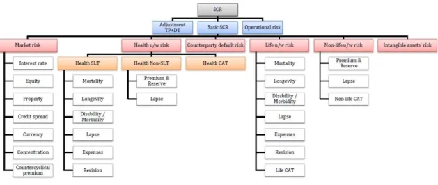
Furthermore, the European standard formula given by the directive uses a modular approach where the risk modules are in turn built on sub-modules (Fig. A.1, Appendix A.3). The SCR for each risk is calculated by re-evaluating best estimate (BE) liabilities (Directive 2009/138/EC, Article 77º) under a specific stress scenario and corresponds to the variation of the basic own funds. These are then aggregated to arrive at the overall SCR, using the so-called square-root formula:

SCR=sX

ij

Corrij ×SCRi×SCRj (4.1.1)

where Corrij represents the correlation factor between risks i and j, given on EIOPA (2014b) (Table A.1, Appendix A.3). EIOPA is the European Insurance and Occupational Pensions Authority.

In order to refine the methodologies, parameters and assumptions, and to help determ-ining the quantitative requirements for new solvency rules, several quantitative impact studies (QIS) have been carried out by EIOPA since 2005. The QIS are the primary means for testing the design of the future European Standard Formula, as well as the main route for finding the correct calibration reflecting the VaR 99.5% over a 1-year time horizon. In preparing the insurance market for the entry into force of the new solvency regime, the ISP (Circular N.º 1/2014) launched a mandatory quantitative impact study nationwide, aimed at all companies under to its prudential supervision.

In this work, the focus is on the biometric risks such as mortality risk (mort), longevity risk (long) and disability or morbidity risk (dis). The Solvency II stress scenarios used to quantify these risks, presented in (EIOPA, 2014b), are the following:

- 15% increase in mortality rates for each age for SCRmort; - 20% decrease in mortality rates for each age for SCRlong;

- 35% increase in disability rates for the next year, together with a permanent 25% increase in disability rates at each age in following years, plus (when applicable) a permanent 20% decrease in morbidity/disability recovery rates.

Under Solvency II the worst-case for the insurer, i.e. the largest value of future obligations, corresponds to the BE plus the SCR obtained from these set of stressed scenarios.

(35)

As a matter of fact, for an insurance company that wishes to exchange the standard SCR by an internal model-based calculation, or simply intends to study the adequacy of the standard formula to its risk profile, the worst-case scenario method presented can show how such "internal stress scenarios" can be derived.

In the next section all the previous elements will be illustrated and applied in order to show how theory and practice may be so harmoniously combined. The situations in ana-lysis, although particular, are at the same time profound and allow us to derive significant conclusions.

4.2 Case Study 1

We start with the policy used by Christiansen (2010) in example 5.1 in order to discuss the impact of using:

- the Portuguese mortality basis: Case Study (CS) 1.1;

- the term structure of interest rates (TSIR) (Brigo and Mercurio, 2006) to discount cash-flow and calculate premiums: CS 1.2.

After that, in CS 1.3, we change the term and the amount of the benefits to amounts more realistic. Lastly, we study two new products with extra covers:

- the disability cover in CS 1.4; - the survival cover in CS 1.5.

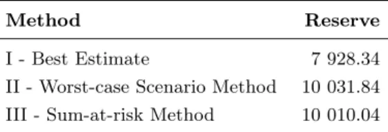
For the different situations described, we present three methods: I - the BE for the reserve (c.f. section 4.1); II - the worst-case method using the discrete time approach Algorithm 3.3.5; III - the sum-at-risk method defining the transition intensity equal to the lower bound where the sum-at-risk with respect to the BE is negative and equal to the upper bound where it is positive (sub-section 3.2.1).

4.2.1 CS 1.1 and CS 1.2

Consider a 30 year old man who buys a policy on 31 December 2013 with the following benefits:

- Ba(t) = 1, t≥67: a pension of 1 is paid yearly in advance from age 67 on till death; - bad(t) = 17, t ∈ {31,32, ...,87}: a sum insured of 17 is paid in case of death before age 87.

(36)

Financial Basis: Under Solvency II, cash-flows should be discounted using the relevant TSIR (Directive 2009/138/EC, Article 77.º). During EIOPA 2014 Stress Test Exercise, EIOPA (2014a) provided a curve for Portugal (Fig. A.6, Appendix A.4).

In order to measure the impact of financial basis we considered the following situations:

CS 1.1 Flat term structure: An interest rate of 2.25%is used in premiums and reserve calculations (Christiansen, 2010);

CS 1.2 TSIR:The risk-free interest rate term structure provided by EIOPA (2014a) is used to discount the reserve from one period to the previous one: ν(t−1, t)

in (3.3.9). As in real practice, premiums are computed using a constant technical interest rate, we assume that it is equal to the internal rate implicit in all outflows discounted using the zero coupon curve plus a bonus factor of 0.5%. The obtained rate is 3.796%.

As usual, the annual premium is paid in advance till retirement or death, whichever occurs first, and is computed using the equivalence principle method and the BE mortality basis. The results are in Table 4.1.

CS 1.1 - Flat Structure CS 1.2 - TSIR

Premium 0.39639 0.26208

Technical Interest Rate 2.25% 3.796%

Table 4.1: CS 1.1 and CS 1.2 - Premiums and technical interest rates

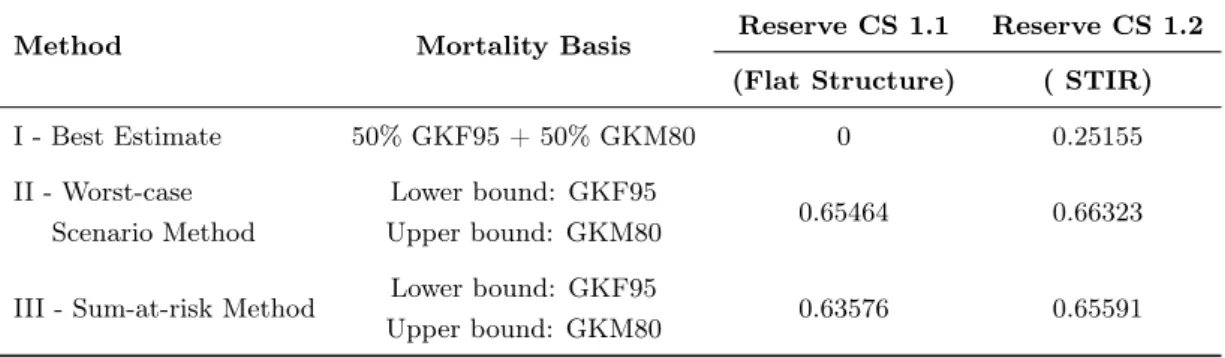
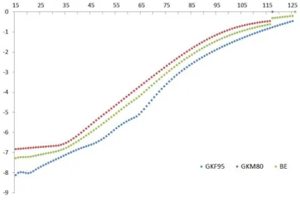
As might be expected, the resulting premiums are different from the one obtained by Christiansen (2010): 0.390147. The new mortality basis has a small positive impact on premiums (CS 1.1) given the highest mortality rates of Swiss BE (Fig. A.4, Appendix A.4). It becomes more significant when combined with the negative interest rate impact (CS 1.2). Table 4.2 shows the reserve at contract time0−, i.e., at age 30−, in state active Va(0−)

for the three different methods.

Method Mortality Basis Reserve CS 1.1 Reserve CS 1.2

(Flat Structure) ( STIR)

I - Best Estimate 50% GKF95 + 50% GKM80 0 0.25155

II - Worst-case Lower bound: GKF95

0.65464 0.66323

Scenario Method Upper bound: GKM80

III - Sum-at-risk Method Lower bound: GKF95 0.63576 0.65591 Upper bound: GKM80

Table 4.2: CS 1.1 and CS 1.2 - Prospective reserveVa 0−

(The results obtained by the author under each of the previous methods are0,1.1647and

(37)

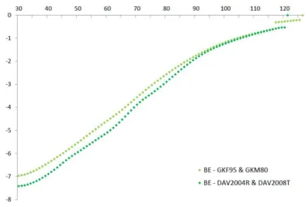
In CS 1.1, the BE is null because the premiums basis is equal to the valuation basis. In order to analyse the impact of using the Portuguese mortality basis, we observe that the life table GKF95 is less conservative than DAV2004R for annuities, while GKM80 is more conservative than DAV2008T until age 83 for policies with occurrence character (Fig. A.3, Appendix A.4). Thus, given the mixed character of the policies in study, the application of Swiss life tables leads always to lower reserves, even when we use GKF95 and GKM80 separately. Further, even using the most conservative of these tables instead of the worst-case or the sum-at-risk methods may underestimate the risk of mortality changes.

If we use the TSIR, the BE is greater than zero, meaning the insurer expects to make a loss on this policy from the outset. It sounds uncomfortable but is not uncommon in practice, explained by the fact that valuation basis may be more conservative than the premium basis. The introduction of the term structure of interest rate leads to an increase in the reserves, under the three methods.

In both situations, the worst-case scenario method required the highest reserve pointing out that although the stress scenarios seem quite demanding that is not necessarily the case. From now one, we will consider the Swiss life tables and the TSIR as the applicable basis.

4.2.2 CS 1.3, CS 1.4 and CS 1.5

Now, consider that the policy was bought by a 35 year old man and the products purchased are as follows.

CS 1.3: Whole life Annuity and Temporary Insurance

- Ba(t) = 14 000, t≥66: a pension of 14 000is paid yearly in advance from age 66 (the retirement age in Portugal for the year 2014) till death;

- bad(t) = 200 000, t ∈ {39,40, ...,75}: a sum insured of 200 000 is paid in case of death before age 75, after a deferred period of 3 years during which no benefits are paid.

CS 1.4: Whole life Annuity and Temporary Insurance with Disability Benefits

Death benefits are the same as in CS 1.3 provided that the disability benefit has not already been paid; There is also a disability benefit: bai(t) = 150 000, t ∈ {37,38, ...,66}: a sum insured of 150 000 is paid in case of permanent disability before age 66, after a deferred period of 1 year during which no benefits are paid.

CS 1.5: Whole life Annuity and Endowment Insurance with disability Benefits

Benefits as in CS 1.4. Now the survival cover at age 75 isBa(75) = 14 000 + 25 000, provided that the life is able at that time.

(38)

Disability basis: According to ISP (2013), disability tables are often given by reinsurers. Thus, we take the Swiss Re 2001 as the lower bound△Lai and the Individual TPD Refer-ence Table of Swiss Re (TPD) as the upper bound△Uai in (3.3.8), and again seems to be reasonable to consider as BE(50%SwissRe2001 + 50%T P D) (Fig. A.5, Appendix A.4). As the maximum age in both tables is 64, we assume that disability rate at age 65 is equal to that at age 64 since the disability rates are already stabilised.

The annual premium is paid in advance till retirement, disability or death, whichever occurs first. The results are in Table 4.3.

CS 1.3 CS 1.4 CS 1.5

Premium 3 833.71 3 942.14 4 127.15

Technical Interest Rate 3.657% 3.632% 3.638%

Table 4.3: CS 1.3, 1.4 and 1.5 - Premiums and technical interest rates

As expected, the introduction of a new cover leads to an increase in premiums.

Table 4.4 present the reserves in state active at time0− under the three usual methods.

Method Mortality Basis Disability Basis

I - Best Estimate 50% GKF95 + 50% GKM80 50% SwissRE2001 + 50% TPD

II - Worst-case Lower bound: GKF95 Lower bound: SwissRe2001 Scenario Method Upper bound: GKM80 Upper bound: TPD

III - Sum-at-risk Method Lower bound: GKF95 Lower bound: SwissRe2001 Upper bound: GKM80 Upper bound: TPD

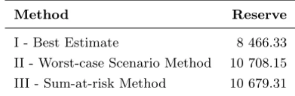
Method CS 1.3 CS 1.4 CS 1.5

I - Best Estimate 2 740.59 2 436.05 2 620.86 II - Worst-case Scenario Method 11 276.00 10 445.34 10 240.43 III - Sum-at-risk Method 11 099.97 10 289.12 9 978.43

Table 4.4: CS 1.3, 1.4 and 1.5 - Prospective reserveVa 0−

Naturally, the introduction of the new covers produces changes in the BE reserve. This is explained by the change in technical interest rate that leads to an increase in premiums. If we consider the same interest rate of3.657% in premiums calculations, the reserve will always increase to2 854.23 and 2 964.18in CS 1.4 and 1.5.

(39)

Appendix A.4). The use of it instead of the worst-case method does not guarantee that we are on the safe side and may underestimate the risk of biometric rate changes.

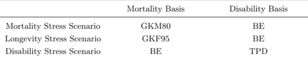
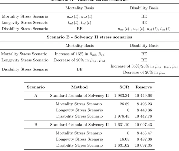
From now on focus is on CS 1.5. Consider the "internal stress scenarios" based on our confidence bands (sub-section 4.2.1) and the Solvency II stress scenarios presented in EIOPA (2014b). EIOPA (2014b, SCR.7.12.) suggests that for policies providing benefits both in case of death and survival, contingent on the life of the same insured person, the mortality and longevity scenarios should be applied to the policy as a whole without decomposing it into the annuity and the life insurance. Therefore, after obtaining the stress scenarios and calculating the SCR’s, they are aggregate with the "square-root formula" using the correlation factors in matrix Table. A.1, Appendix A.3. Table 4.5 summarizes the results.

Scenario A-Internal stress scenarios

Mortality Basis Disability Basis

Mortality Stress Scenario GKM80 BE

Longevity Stress Scenario GKF95 BE

Disability Stress Scenario BE TPD

Scenario B - Solvency II stress scenarios

Mortality Basis Disability Basis

Mortality Stress Scenario Increase of 15% in BE BE Longevity Stress Scenario Decrease of 20% in BE BE

Disability Stress Scenario BE Increase of 35%/ 25% in BE

Scenario Method SCR Reserve

A Standard formula of Solvency II 1 698.97 4 319.83

Mortality Stress Scenario 1 467.06 4 087.92 Longevity Stress Scenario 1 276.71 3 897.57 Disability Stress Scenario 51.87 2 672.73

B Standard formula of Solvency II 653.85 3 274.70

Mortality Stress Scenario 68.49 2 689.35 Longevity Stress Scenario 514.53 3 135.39 Disability Stress Scenario 402.40 3 023.26

Table 4.5: CS 1.5 - Standard formula of Solvency II

Observe that while the prevailing risk in scenario A is the mortality risk, in scenario B is the longevity risk. Remembering that the worst-case scenario (Table 4.4) requires a reserve of10 240.43, the value obtained in scenario A is lower and a possible explanation is that although the square-root formula considers the correlation between the risks, it disregards mixed mortality scenarios. Furthermore, according to Theorem 3.3.2 scenarios

¯

II E UNICEA LEXANDRAM ADEIRAB ALAU

M

ASTER IN

A

CTUARIAL

S

CIENCE

M

ASTERS

F

INAL

W

ORK

DISSERTATION

P

REMIUMS AND

R

ESERVES IN

L

IFE

I

NSURANCE

P

OLICIES:

T

HE

W

ORST-CASE

S

CENARIO AND

S

OLVENCY

II

EUNICE

ALEXANDRA

MADEIRA

BALAU

M

ASTER IN

A

CTUARIAL

S

CIENCE

M

ASTERS

F

INAL

W

ORK

DISSERTATION

P

REMIUMS AND

R

ESERVES IN

L

IFE

I

NSURANCE

P

OLICIES:

T

HE

W

ORST-CASE

S

CENARIO AND

S

OLVENCY

II

EUNICE

ALEXANDRA

MADEIRA

BALAU

SUPERVISOR:

PROF.

ONOFRE

ALVES

SIMÕES

Contents

List of Figures

_{REMIUMS AND}

_{ESERVES IN}

_IFE

_NSURANCE

_OLICIES:

_HE

_ORST-CASE

_{CENARIO AND}

_OLVENCY

_{REMIUMS AND}

_{ESERVES IN}

_IFE

_NSURANCE

_OLICIES:

_HE

_ORST-CASE

_{CENARIO AND}

_OLVENCY