Infinite servers queue systems computational simulation

Texto

(1)INFINITE SERVERS QUEUE SYSTEMS COMPUTATIONAL SIMULATION FERREIRA Manuel Alberto M. (P), ANDRADE Marina (P) Abstract. For many parameters of interest in the study or application of queuing systems either there are not theoretical results or, existing, they are very complicated what makes their utility doubtful. In this situation it is very common to use simulation methods in order to get useful results. Here a Fortran program to simulate infinite servers queuing systems is presented. Through it, some experiences are performed and the respective results are used to conjecture about some interesting quantities of those systems, mainly about the busy period. Keywords: Infinite servers queue systems, simulation, busy period Mathematics Subject Classification: 60G99. 1. Introduction. The absence of theoretical results, often difficult to obtain, or its extreme complexity that makes its utility doubtful, leads to the search for numerical methods, in particular simulation methods, in the study of queue systems. The objective in this work is to do so for queue systems with infinite servers. The most known and studied of these systems is the M / G / ∞ queue. For it a lot of results are known and result very clear and simple to use, see for example (Carrillo, 1981), (Ferreira, 2002) and (Ferreira and Andrade, 2009, 2010, 2010a, 2010b, 2011, 2012). One of the situations simulated in this work is related to the consideration of non-Poisson arrivals that is with inter-arrival times not exponential for which there are no analytical results. Other results collected are about the busy period1, for Poisson and non-Poisson arrivals. In fact any queue system has a sequence of busy periods and idle periods. A busy period followed by an idle period is a busy cycle. In the study of infinite servers systems busy periods very useful information is, for instance, about the maximum number of customers served simultaneously in a busy period. If something is known about this quantity the system may be dimensioned as a finite servers queue. As there are not analytical results the simulation is one of the issues to study it.. 1. A busy period begins with the arrival of a customer to the system, being it empty, ends when a customer abandons the system, letting it empty, and there is always at least one customer in the system.. 1.

(2) In the next section, details about the FORTRAN program built to perform the simulations and the experiences performed are presented. The following section consists in the presentation of the results and the respective comments. The paper ends with a conclusions section. 2. The Computational Simulation. The simulations were performed using a Fortran program, see Appendix, composed of: i) A main program, in Fortran language, called FILAESP, ii) A subroutine GERASER, iii) A package SSPLIB iv) A function system RAN. The proceedings are as follows: i) The sequential random generation of 25 000 arrivals instants, being the inter- arrivals mean time 0.99600, ii) The generation of 25 000 service times that are added to the arrivals instants so obtaining the departure instants, iii) The ordination of the arrivals and departure instants, through an ordination algorithm making to correspond to each arrival 1 and to each departure -1, iv) The generation, in fact, of the queue summing by order those values 1 and -1, in correspondence with the instants at which they occur, v) The processing of the information of iv) in order to obtain a) Data related to the state of the system2: • Number of the visits to the assumed states, • Mean sojourn time in each one of those states. b) Data related to the busy period: • • •. The maximum number of customers served simultaneously in a busy period, Total number of customers served in the busy period, Length of the busy period.. The arrivals instant generation is performed in the program FILAESP and the service times in the GERASER subroutine. The arrivals and departures instants ordination is performed in the program FILAESP through the SSPLIB package. The construction of the queue and the processing of the information occur also in FILAESP. In the generation of the arrivals and the departures are used sequences of pseudo-random numbers supplied by the system function RAN. In general it is made RAN(E*J), being E constant in each experience and assuming J the values from 1 to 25 000. E was chosen to be an integer with four digits. 2. The state of the system, in a given instant, is the number of customers that are being served in that instant.. 2.

(3) To the arrivals process one or two sequences of pseudo-random numbers are needed as considering M, exponential inter-arrival times, or E2, Erlang with parameter 2 inter-arrival times. In the first case it must be made an option for an integer with four digits, E, and in the second for two integers with four digits that will be designated by E and by F. The same happens with the service distribution, considering so G or G and H, as working with M or E2. The experiences performed are described below, being traffic intensity. -. M/M/∞ E = 7 528 F = 7 548 4 4.016 Number of observed busy periods: 208. -. M/M/∞ E = 7 529 F = 7 549 5 5.020 Number of observed busy periods: 28. -. M / E2 / ∞ E = 7 528 G = 7 552 H = 6 666 4 4.016 Number of observed busy periods: 337. -. M / E2 / ∞ E = 7 529 G = 6 552 H = 6 667 5 5.020 Number of observed busy periods: 69. -. E2 / E2 / ∞ E = 4 536 F = 4 537 G = 5 224 H = 6 225 4 4.016 Number of observed busy periods: 804. 3. the mean service time and. the.

(4) E2 / E2 / ∞ E = 4 538 F = 4 539 G = 5 228 H = 6 229 5 5.020 Number of observed busy periods: 208. -. The mean service times considered, 4 and 5, were those for which a reasonable number of busy periods was obtained, among the highest. In fact, increasing the mean service time the observed busy periods decrease very quickly. Note that for the systems M / M / ∞ and M / E2 / ∞, for the same values of generated are identical. 3. the arrivals instants. The Results – Presentation and Comments. In Figure 1 and Figure 2 the graphics that represent the mean sojourn times in the various states3, for the M / M / ∞ system, considering ρ = 4.016 and ρ = 5.020, respectively, are presented. Beyond the observed mean values the theoretical values are also presented, see (Ramalhoto, 1983), given by ,. 0, 1, 2, …. (1). In correspondence with the various states are also indicated the number of times that they were visited, in the right columns. 1,2 1 0,8. Theoretical Mean Sojourn Times in state i=0,1, 2,3,4,5,6,7,8,9,10,11 Observed Mean Sojourn Times in state i=0,1,2,3,4,5,6,7,8,9,10,11. 0,6 0,4 0,2 0 0 1 2 3 4 5 6 7 8 9 10 11 12. state 0 1 2 3 4 5 6 7 8 9 10 11. visits 247 2018 5970 9624 10339 8809 6106 3581 2132 961 205 7. Figure 1. Mean Sojourn Times, in seconds, theoretical and observed, for the M / M / ∞ queue system in states i = 0, 1, …, 11, with ρ = 4.016.. 3. The state of the system in a given instant is the number of costumers that are being served in that instant.. 4.

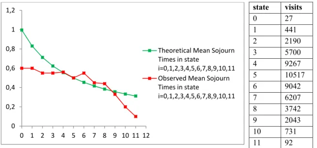
(5) 1,2 1 0,8. Theoretical Mean Sojourn Times in state i=0,1,2,3,4,5,6,7,8,9,10,11 Observed Mean Sojourn Times in state i=0,1,2,3,4,5,6,7,8,9,10,11. 0,6 0,4 0,2 0 0 1 2 3 4 5 6 7 8 9 10 11 12. state 0 1 2 3 4 5 6 7 8 9 10 11. visits 27 441 2190 5700 9267 10517 9042 6207 3742 2043 731 92. Figure 2. Mean Sojourn Times, in seconds, theoretical and observed, for the M / M / ∞ queue system in states i = 0, 1, …, 11, with ρ = 5.020.. In Figure 3 and Figure 4 are shown the distributions obtained for the number of customers in the systems M / M / ∞, M / E2 / ∞ and E2 / E2 / ∞ with ρ = 4.016 and ρ = 5.020, respectively. Together is also presented the theoretical distribution, in equilibrium, for the systems M / M / ∞ and M / E2 / ∞, see (Tackács, 1962): !. ,. 0, 1, 2, …. (2). Performing the direct computations for ρ = 4.016 and ρ = 5.020. E[N] is the mean number of customers in the system. 0,25. 0,2 Theoretical Distribution. 0,15. M/M/Inf; E[N]=4.366 M/E2/Inf; E[N]=4.368. 0,1. E2/E2/Inf; E[N]=4.376 0,05. 0 0 1 2 3 4 5 6 7 8 9 10 11 12. Figure 3. Distribution of the Number of Customers in the System and Theoretical Distribution for the Systems M / M / ∞, M / E2 / ∞ and E2 / E2 / ∞ with ρ = 4.016.. 5.

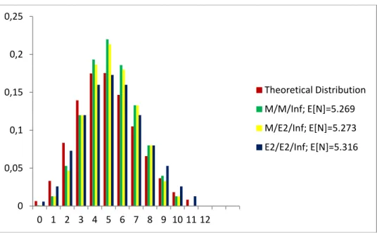
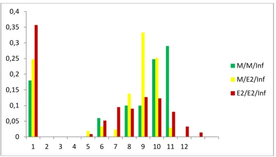
(6) 0,25. 0,2 Theoretical Distribution. 0,15. M/M/Inf; E[N]=5.269 M/E2/Inf; E[N]=5.273. 0,1. E2/E2/Inf; E[N]=5.316 0,05. 0 0 1 2 3 4 5 6 7 8 9 10 11 12. Figure 4. Distribution of the Number of Customers in the System and Theoretical Distribution for the Systems M / M / ∞, M / E2 / ∞ and E2 / E2 / ∞ with ρ = 5.020.. These Figures suggest some similarity of behaviour among the empirical distributions and the theoretical distribution. Particularly, in the whole of them the mode is identical to the one of the theoretical distribution. But although for the systems M / M / ∞ and M / E2 / ∞ the empirical distributions are more concentrated around the mode, in comparison with the theoretical distribution, the opposite happens to the system E2 / E2 / ∞. And, surprisingly because for this system it is not known the theoretical distribution, the empirical distributions obtained for E2 / E2 / ∞ seems closer to the theoretical distribution than the ones of the other systems. As for the differences observed between the systems M / M / ∞ and M / E2 / ∞, for the number of the customers in the system, the adequate interpretation may be as follows: although the systems reach certainly the equilibrium, since the number of the simulated arrivals is quite large there is a strong presence of an initial transitory trend that must last a long time. Note, observing Figure 1 and Figure 2, that the mean sojourn times observed and theoretical, given by (1), for the system M / M / ∞ are quite close. This closeness is better for the states to which corresponds greater frequency. In Figure 5 and Figure 6, about the maximum number of customers served simultaneously in the busy period, it is remarked great diversity in the distributions form. It is always observed a great frequency for the state 1. In the E2 / E2 / ∞ infinite systems it is always the mode. Curiously, these systems being able to serve any number of customers, present, in these simulations, few customers being served simultaneously: never above the number 14, only assumed by the E2 / E2 / ∞ infinite systems. This fact is acceptable, in terms of the theoretical distribution, since in the Poisson distribution the values greater than the mode, far away from it, are little probable. Note still that, excluding from this analysis the state 1, the distributions of maximum number of customers served simultaneously in the E2 / E2 / ∞ infinite systems busy period are more scattered than those of the others. This is in accordance with the fact that, for the same number of arrivals, much more busy periods are observed for the E2 / E2 / ∞ infinite systems.. 6.

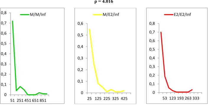
(7) 0,4 0,35 0,3 0,25. M/M/Inf. 0,2. M/E2/Inf. 0,15. E2/E2/Inf. 0,1 0,05 0 1. 2. 3. 4. 5. 6. 7. 8. 9. 10 11 12. Figure 5. Distribution of the Maximum Number of Customers Served Simultaneously in a Busy Period for the Systems M / M / ∞, M / E2 / ∞ and E2 / E2 / ∞ with ρ = 4.016.. 0,4 0,35 0,3 0,25. M/M/Inf. 0,2. M/E2/Inf. 0,15. E2/E2/Inf. 0,1 0,05 0 1. 2. 3. 4. 5. 6. 7. 8. 9. 10 11 12. Figure 6. Distribution of the Maximum Number of Customers Served Simultaneously in a Busy Period for the Systems M / M / ∞, M / E2 / ∞ and E2 / E2 / ∞ with ρ = 5.020.. Figure 7 suggests a more and more smooth behaviour of the busy period lengths distribution frequency curve when going from M / M / ∞ system for the M / E2 / ∞ system and then for the E2 / E2 / ∞ system. The whole of them present a great frequency concentration for the lowest values of the busy period lengths but, in the case of M / M / ∞ system, the interval along which the observations spread has more than the double of the length of the other systems. Remember, again, that for the M / M / ∞ system much less busy periods are observed than for the M / E2 / ∞ system and, for this one less than for the E2 / E2 / ∞ system. Then the curve of frequencies for the M / M / ∞ system spreads along that interval with two deep valleys. The one of the M / E2 / ∞ system presents also two valleys, but less deep, and in E2 / E2 / ∞ system practically they are not observed. Note, also that those valleys occur for different values in the M / M / ∞ and M / E2 / ∞ systems. 7.

(8) ρ = 4.016 0,8. M/M/Inf. M/E2/inf. 0,7. 0,6. 0,6. 0,5. E2/E2/Inf 0,8 0,7 0,6. 0,5. 0,4. 0,4. 0,5 0,4. 0,3. 0,3. 0,3. 0,2 0,2. 0,2 0,1. 0,1. 0,1 0. 0. 0. 53 123 193 263 333. 25 125 225 325 425. 51 251 451 651 851. Figure 7. Distribution of Observed Busy Period Lengths, in seconds, for the Systems M / M / ∞, M / E2 / ∞ and E2 / E2 / ∞ with ρ = 4.016.. ρ = 5.020 0,6. M/M/Inf. 0,5 0,4 0,3 0,2 0,1. M/E2/inf 0,5. 1. 0,45. 0,9. 0,4. 0,8. 0,35. 0,7. 0,3. 0,6. 0,25. 0,5. 0,2. 0,4. 0,15. 0,3. 0,1. 0,2. 0,05. 0,1 0. 0. 0 310. 2170 4030. E2/E2/Inf. 105 525 945 1365. 40 200 360 520. Figure 8. Distribution of Observed Busy Period Lengths, in seconds, for the Systems M / M / ∞, M / E2 / ∞ and E2 / E2 / ∞ with ρ = 5.020.. Figure 8 suggests a greater similarity among the busy period lengths distributions of the various systems. Again it is observed a great concentration in the lowest values although lesser that in Figure 7. But now the whole of them present one valley, although for different values. Still goes on observing a great disparity among the maximum values assumed by the busy period lengths.. 8.

(9) It seems evident, either in Figure 7 or in Figure 8, a sharp observations lack in the intermediate values zone for the busy period lengths. Note also that the Figures 7 and 8 are in accordance with the studies that point in order that the busy period length distribution of the M / G / ∞ system is right asymmetric and leptokurtic see (Ferreira and Ramalhoto, 1994). ρ = 4.016. ρ = 5.020. 12. 9 8 7 6 5 4 3 2 1 0 ‐1. 10 8. M/M/Inf; R=0.98. 6 4. M/E2/inf; R=0.94. 2. E2/E2/Inf ; R=0.93. 0 ‐2. 1 3 5 7 9 11 13. M/M/Inf; R=0.97 M/E2/Inf; R=0.96 E2/E2/Inf; R=0.92 1 3 5 7 9 11 13. Figure 9. Regression of Z over X, for the Systems M / M / ∞, M / E2 / ∞ and E2 / E2 / ∞ with ρ = 4.016 and ρ = 5.020. R is the Linear Coefficient Regression.. Call X and Y the maximum number of customers served simultaneously and the total number of served customers, respectively, in the busy period. Performing the regression of Z = lnY on X. The results obtained are presented graphically in Figure 9 and the most interesting fact is, maybe the similarity of the lines behaviour, for the various systems, for the two values of ρ considered. The systems for which more busy periods are observed – and, so, also with lesser lengths – are those to which correspond greater values of . But, for each system there is a great resemblance of the values of and for the two values of ρ considered. In fact, it seems natural that the relation between Z and X does not depend on ρ. The values of ρ will only influence the values of Z and X that may occur and not the relation between them. Otherwise, will it be true that the difference observed between the values of and for the various systems, not being too great, allows to face the hypothesis of that the relation between Z and X is identical for those systems? Maybe yes if we pay attention to the similarities of observed in its behaviour, namely the ones related with the distribution of the number of customers in the systems. 4. Conclusions. It is evident the great waste of these systems when looking to the maximum number of customers present simultaneously in the system. It is uncontroversial, also, that there is a strong exponential relation between the maximum number of customers served simultaneously in a busy period and the total number of served customers. The. 9.

(10) question is if either it is always the same or how will it change either with the values of ρ or from system to system. About the busy period it is important to note also: i) The great occurrence of busy periods with only one served customer, ii) The great amplitude of the interval at which occur the values of the lengths of the busy periods, although with a great irregularity, and a great occurrence of low values. The results of these simulations seem to suggest also that the systems GI /G / ∞ may be quite well approximated by systems M / G / ∞, at least when the GI process possesses a regularity not very far from the one of the Poisson process. Acknowledgement This work was financially supported by FCT through the Strategic Project PEst-OE/EGE/UI0315/2011. References [1] Andrade, M.: A Note on Foundations of Probability. Journal of Mathematics and Technology, vol.. 1, No 1, pp 96-98, 2010. [2] Carrillo, M. J.: Extensions of Palm’s Theorem: A Review. In Management Science, Vol. 37, No 6, pp. 739-744, 1991. [3] Ferreira, M. A. M.: Simulação de variáveis aleatórias – Método de Monte Carlo. Revista Portuguesa de Gestão, I (III/IV), pp. 119-127. ISCTE, 1994. [4] Ferreira, M. A. M.: Application of Ricatti Equation to the Busy Period Study of the M⏐G⏐∞ System. In Statistical Review, 1st Quadrimester, INE, pp. 23-28, 1998. [5] Ferreira, M. A. M.: Computational Simulation of Infinite Servers Systems. In Statistical Review, 3rd Quadrimester, INE, pp. 5-28, 1998a. [6] Ferreira, M. A. M.: M⏐G⏐∞ Queue Heavy-Traffic Situation Busy Period Length Distribution (Power and Pareto Service Distributions). In Statistical Review, 1st Quadrimester, INE, pp. 27-36, 2001. [7] Ferreira, M. A. M.: The Exponentiality of the M⏐G⏐∞ Queue Busy Period. In Actas das XII Jornadas Luso-Espanholas de Gestão Científica, Volume VIII- Economia da Empresa e Matemática Aplicada. UBI, Covilhã, Portugal. pp. 267-272, 2002. [8] Ferreira, M. A. M. and Andrade, M.: The Ties Between the M/G/∞ Queue System Transient Behaviour and the Busy Period. In International Journal of Academic Research Vol. 1, No 1, pp. 84-92, 2009. [9] Ferreira, M. A. M. and Andrade, M.: Looking to a M/G/∞ system occupation through a Ricatti equation. In Journal of Mathematics and Technology, Vol. 1, No 2, pp. 58-62, 2010. [10] Ferreira, M. A. M. and Andrade, M.: M/G/∞ System Transient Behavior with Time Origin at the Beginning of a Busy Period Mean and Variance. In Aplimat- Journal of Applied Mathematics, Vol. 3, No 3, pp. 213-221, 2010a.. 10.

(11) [11] Ferreira, M. A. M. and Andrade, M.: M/G/∞ Queue Busy Period Tail. In Journal of Mathematics and Technology, Vol. 1, No 3, 11-16, 2010b. [12] Ferreira, M. A. M. and Andrade, M.: Fundaments of Theory of Queues. International Journal of Academic Research, Vol. 3, No 1, part II, pp. 427-429, 2011. [13] Ferreira, M. A. M. and Andrade, M.: Busy Period and Busy Cycle Distributions and Parameters for a Particular M/G/oo queue system. American Journal of Mathematics and Statistics, Vol. 2, No 2, pp. 10-15, 2012. [14] Ferreira, M. A. M. and Ramalhoto M. F.: Estudo dos parâmetros básicos do Período de Ocupação da Fila de Espera M⏐G⏐∞. In A Estatística e o Futuro da Estatística. Actas do I Congresso Anual da S.P.E.. Edições Salamandra, Lisboa, 1994. [15] Ferreira, M. A. M., Andrade, M. and Filipe, J. A.: The Ricatti Equation in the M⏐G⏐∞ Busy Cycle Study. In Journal of Mathematics, Statistics and Allied Fields Vol. 2, No 1, 2008. [16] Ferreira, M. A. M., Andrade, M. and Filipe, J. A.: Networks of Queues with Infinite Servers in Each Node Applied to the Management of a Two Echelons Repair System. In China-USA Business Review Vol. 8, No 8, pp. 39-45 and 62, 2009. [17] Figueira, J. and Ferreira, M. A. M.: Representation of a Pensions Fund by a Stochastic Network with Two Nodes: An Exercise. In Portuguese Revue of Financial Markets, Vol. I, No 3, 1999. [18] Hershey, J. C., Weiss, E. N. and Morris, A. C.: A Stochastic Service Network Model with Application to Hospital Facilities. In Operations Research, Vol. 29, No 1, pp. 1-22, 1981. [19] Kelly, F. P.: Reversibility and Stochastic Networks. New York: John Wiley and Sons, 1979. [20] Kendall and Stuart: The Advanced Theory of Statistics. Distributions Theory. London. Charles Griffin and Co., Ltd. 4th Edition, 1979. [21] Kleinrock, L.: Queueing Systems. Vol. I and Vol. II. Wiley- New York, 1985. [22] Metropolis, N. and Ulan, S.: The Monte Carlo Method. Journal of American Statistical Association, Vol. 44, No 247, pp. 335-341, 1949. [23] Murteira, B.: Probabilidades e Estatística,. Vol. I. Editora McGraw-Hill de Portugal, Lda. Lisboa, 1979. [24] Ramalhoto, M. F.: A Note on the Variance of the Busy Period of the M⏐G⏐∞ Systems. Centro de Estatística e Aplicações, CEAUL, do INIC and IST. 1983. [25] Stadje, W.: The Busy Period of the Queueing System M⏐G⏐∞. In Journal of Applied Probability, Vol. 22, pp. 697-704, 1985. [26] Syski, R.: Introduction to Congestion Theory in Telephone Systems, Oliver and BoydLondon, 1960. [27] Syski, R.: Introduction to Congestion Theory in Telephone Systems. North Holland. Amsterdam, 1986. [28] Tackács, L.: An Introduction to Queueing Theory. Oxford University Press. New York, 1962.. 11.

(12) Current address Manuel Alberto M. Ferreira, Professor Catedrático INSTITUTO UNIVERSITÁRIO DE LISBOA (ISCTE-IUL) BRU - IUL AV. DAS FORÇAS ARMADAS 1649-026 LISBOA, PORTUGAL TELEFONE: + 351 21 790 37 03 FAX: + 351 21 790 39 41 E-MAIL: manuel.ferreira@iscte.pt Marina Andrade, Professor Auxiliar INSTITUTO UNIVERSITÁRIO DE LISBOA (ISCTE-IUL) BRU - IUL AV. DAS FORÇAS ARMADAS 1649-026 LISBOA, PORTUGAL TELEFONE: + 351 21 790 34 05 FAX: + 351 21 790 39 41 E-MAIL: marina.andrade@iscte.pt. 12.

(13) Appendix PROGRAM FILAESP C C. 555 666 100. 500. 600. 650. APAGUE 666 OU 555 CONFORME QUEIRA TEMPO INTERCHEGADAS EXPONENCIAL OU ERLANG DE PARAMETRO 2 DIMENSION V(25000),Y1(25000),Y2(25000),TEPSER(25000) DIMENSION C(25000),AUX(50000),P(25000),N(50000),F(50000) DIMENSION Z(50000),VAL(50000),ARG(50000) DIMENSION NO(0:50000),T(0:25000),TM(0:25000) DIMENSION TTR(0:25000),TMR(0:25000) DIMENSION BUPE(0:25000),NA(0:25000) WRITE(*,*)’O CODIGO DOS SERVICOS E: 0 PARA A PARETO, 1 PARA A’ WRITE(*,*)’EXPONENCIAL, 2 PARA A ERLANG, 3 PARA A LOGNORMAL,’ WRITE(*,*)’4 PARA A MISTURA DE EXPONENCIAIS COM RPARAMETRO,’ WRITE(*,*)’5 PARA A MISTURA DE ERLANG.’ WRITE(*,*)’ ’ WRITE(*,*)’ QUAL E O CODIGO DA DISTRIBUICAO DE SERVICO?’ READ(*,*) ICOD WRITE(*,*)’ ’ WRITE(*,*)’ BOA SORTE NA VIAGEM AO MUNDO DA SIMULACAO ’ WRITE(*,*)’ ’ WRITE(*,*)’ ’ U=0.99600 DO 100 I=1,25000 V(I)=ALOG(RAN(E*I))*(-U/2.0) V(I)=ALOG(RAN(E*I))*(-U/2.0)+ALOG(RAN(F*I))*(-U/2.0) CONTINUE CALL GERASER(TEPSER) C(1)=V(1) Z(1)=C(1) F(1)=1 Z(25001)=V(1)+TEPSER(1) F(25001)=-1 DO 500 I=2,25000 C(I)=C(I-1)+V(I) P(I)=C(I)+TEPSER(I) Z(I)=C(I) F(I)=1 Z(I+25000)=P(I) F(I+25000)=-1 CONTINUE X=0.0 ICOL=1 IROW=50000 NDIM=50000 CALL ATSG(X,Z,F,AUX,IROW,ICOL,ARG,VAL,NDIM) N(1)=1 DO 600 I=2,50000 N(I)=N(I-1)+VAL(I) CONTINUE MAX=1 DO 650 I=2,50000ESTRE DE 1998 IF (N(I).GE.MAX)MAX=N(I) CONTINUE WRITE(10,*)’ SIMULACAO FILA DE ESPERA M|G|∞ ‘ DO 700 K=0,MAX. 13.

(14) 660 1000. 700. 4000. I 3900. WRITE(10,*)’ TEMPOS DE RECORRENCIA DO ESTADO ‘,K J=1 NO(K)=0 T(K)=0.0 TM(K)=0.0 DO 660 I=1,49999 IF(N(I).EQ.K) THEN NO(K)=NO(K)+1 T(K)=T(K)+(ARG(I+1)-ARG(I)) J=J+1 ENDIF CONTINUE DO 1000 J=1,NO(K)-1 TTR(K)=TTR(K) CONTINUE IF(NO(K).NE.0)TM(K)=T(K)/NO(K) IF(NO(K).GT.1)TMR(K)=TTR(K)/(NO(K)-1) IF(NO(K).EQ.1)TMR(K)=0 WRITE(10,*)’ESTADO’,K WRITE(10,*)’NUMERO DE VISITAS =’,NO(K) WRITE(10,*)’TEMPO DE PERMANENCIA =’,T(K) WRITE(10,*)’TEMPO MEDIO DE PERMANENCIA =’,TM(K) WRITE(10,*)’TEMPO TOTAL DE RECORRENCIA =’,TTR(K) WRITE(10,*)’TEMPO MEDIO DE RECORRENCIA =’,TMR(K) CONTINUE TTBUPE=ARG(50000)-ARG(1)-T(0) NTBUPE=1+N0(0) TMBUPE=TTBUPE/NTBUPE TTIDP=T(0) NTIDP=NO(0) TMIDP=TM(0) WRITE(10,*)’NO TOTAL DE PERIODOS DE OCUPACAO =’,NTBUPE WRITE(10,*)’TEMPO TOTAL DE BUSY PERIOD =’,TTBUPE WRITE(10,*)’TEMPO MEDIO DE BUSY PERIOD =’,TMBUPE WRITE(10,*)’NO TOTAL DE PERIODOS DE DESOCUPACAO =’,NTIDP WRITE(10,*)’TEMPO TOTAL DE IDLE PERIOD =’,TTIDP WRITE(10,*)’TEMPO MEDIO DE IDLE PERIOD =’,TMIDP BUPE(0)=0 NA(0)=1 NP=0 DO 5000 I=1,49999 IF(N(I).EQ.0) THEN NP=NP+1 WRITE(10,*)’BUSY PERIOD NUMERO’,NP NA(NP)=I NB=0 DO 4000 J=NA(NP-1),NA(NP)-1 IF(N(J+1).GT.N(J))NB=NB+1 CONTINUE IF(NP.EQ.1)NB=NB+1 WRITE(10,*)’NUMERO DE CLIENTES ATENDIDOS=’,NB MAXI=1 DO 3900 J=NA(NP-1),NA(NP) IF(N(J).GE.MAXI) MAXI=N(J) CONTINUE WRITE(10,*)’NUMERO MAXIMO DE CLIENTES ATENDIDOS SIMULTANEAMENTE=’,MAXI BUPE(NP)=ARG(I+1) RBUPE=BUPE(NP)-BUPE(NP-1)-ARG(I+1)+ARG(I). 14.

(15) 5000. 4001. 4002. IF(NP.EQ.1)RBUPE=BUPE(1)-ARG(I+1)+ARG(I)-ARG(1) WRITE(10,*)’COMPRIMENTO=’,RBUPE ENDIF CONTINUE NP=NP+1 WRITE(10,*)’BUSY PERIOD NUMERO=’,NP NB=0 DO 4001 J=NA(NP-1),49999 IF(N(J+1).GT.N(J))NB=NB+1 CONTINUE IF(NP.EQ.1)NB=NB+1 WRITE(10,*)’NUMERO DE CLIENTES ATENDIDOS=’NB MA=1 DO 4002 J=NA(NP-1),50000 IF(N(J).GE.MA)MA=N(J) CONTINUE WRITE(10,*)’NUMERO MAXIMO DE CLIENTES ATENDIDOS SIMULTANEAMENTE=’MA RBUPE=ARG(50000)-BUPE(NP-1) IF(NP.EQ.1)RBUPE=ARG(50000)-ARG(1) WRITE(10,*)’COMPRIMENTO= ’,RBUPE END SUBROUTINE GERASER (T) DIMENSION T(25000) ICOD=2 IF (ICOD.EQ.0) THEN PRINT*, ‘INTRODUZA O VALOR DO COEFICINTE DE VARIACAO’ READ*,GAMA ALFA=2*GAMA/(GAMA-1.0) RK=E*(GAMA+1.0)/(2*GAMA) ELSEIF (ICOD.EQ.4) THEN PRINT*,’INTRODUZA O VALOR DO PARAMETRO DA MISTURA’ READ(*,*)RPARAMETRO ENDIF IX=35 IY=43 IIX=9 IJX=5 IKX=11 ILX=13 DO 10 I=1,250000 CALL RANDU(IX,IY,FL) IF(ICOD.EQ.O) THEN T(I)=RK/(1-FL)**(1.0/ALFA) ELSE IF (ICOD.EQ.1) THEN T(I)=-7.0*ALOG(RAN(G*I)) ELSE IF (ICOD.EQ.2) THEN T(I)=-(4.0/2.0)*ALOG(RAN(G*I))-(4.0/2.0)*ALOG(RAN(H*I)) ELSE IF (ICOD.EQ.3) THEN CALL RANDU(JX,IJY,YFFL) IJX=IJY T(I)=EXP((-2*ALOG(YFFL))**(0.5)*COS(8*ATAN(1.0)*FL)) ELSE IF (ICOD.EQ.4) THEN CALL RANDU (IKX,IKY,RFL) IKX=IKY CALL RANDU (ILX,ILY,SFL). 15.

(16) 10. ILX=ILY IF (FL.LE.RPARAMETRO) THEN T(I)=-(3.45/2.0)*(1.0/RPARAMETRO)*LOG(RFL) ELSE T(I)=-(3.45/2.0)*(1.0/1.0-RPARAMETRO)*LOG(SFL) ENDIF ELSE IF (ICOD.EQ.5) THEN CALL RANDU (IKX,IKY,RFL) IKX=IKY CALL RANDU (ILX,ILY,SFL) ILX=ILY CALL RANDU (IMX,IMY,TFL) IMX=IMY CALL RANDU (INX,INY,UFL) INX=INY CALL RANDU (IPX,IPY,VFL) IPX=IPY CALL RANDU (IQX,IQY,WFL) IQX=IQY IF(RFL.LT.0.400) THEN T(I)=-((10.0/2.7)/4.0)*(LOG(UFL)+LOG(SFL)+LOG(TFL)+LOG(WFL)) ELSE IF ((RFL.GT.0.4000).AND.(RFL.LT.0.75)) THEN T(I)=-((10.0/4.2)/2.0)*(LOG(VFL)+LOG(WFL)) ELSE IF (RFL.GT.0.75) THEN T(I)=-((10.0/3.6)/3.0)*(LOG(VFL)+LOG(WFL)+LOG(SFL)) ENDIF ENDIF CONTINUE END. 16.

(17)