M
ASTER OF
S
CIENCE IN
F
INANCE
M
ASTERS
F
INAL
W
ORK
D
ISSERTATION
CAPM
FOR
PROJECT
FINANCE
USING
THE
PORTUGUESE
PUBLIC
PRIVATE
PARTNERSHIPS
ROAD
SECTOR
M
ASTER OF
S
CIENCE IN
F
INANCE
M
ASTERS
F
INAL
W
ORK
DISSERTATION
CAPM
FOR
PROJECT
FINANCE
USING
THE
PORTUGUESE
PUBLIC
PRIVATE
PARTNERSHIPS
ROAD
SECTOR
M
IGUEL
F
ERREIRA
N
EVES DE
O
LIVEIRA
S
UPERVISOR:
P
ROFESSOR
J
OAQUIM
M
IRANDA
S
ARMENTO
Average Cost of Capital (WACC), we propose the discussion of the appropriate discount rates for the case of Portuguese public private partnerships (PPPs) in the road sector, namely from the perspective of private sector investors. Calculation of the cost of equity is performed using two different methodologies: a comparable firms approach and with the use of publicly available data (Damodaran Online) on the European transportation sector. Furthermore, we find that the CAPM cost of equity is very dependent on the high leverage of PPP projects. The computed discount rates are later subjected to econometric (OLS) testing, regarding the influence of having a foreign shareholder majority, of the availability payment scheme and of Portuguese Treasury 10 year bond yields (spreads vs. Germany). We find that the appropriate discount rates (WACC) should be in the range of 6 to 8% and that the existence of foreign shareholders is associated with lower project risk and lower costs of equity, at 10% significance level.
Keywords: Public Private Partnerships; CAPM; Discount rate; WACC; Portuguese Road Sector.
Average Cost of Capital (WACC), propõe-se uma discussão das taxas de
desconto apropriadas para as parcerias público-privadas (PPPs) Portuguesas no sector rodoviário, nomeadamente na perspectiva dos investidores privados. O cálculo do custo dos capitais próprios é realizado através de duas metodologias: usando dados de empresas comparáveis e com o uso de dados públicos (Damodaran Online) sobre o setor dos transportes a nível europeu. Para além disso, concluímos que o cálculo do custo dos capitais próprios através do CAPM depende muito dos grandes níveis de alavancagem dos projectos PPP. As taxas de desconto obtidas são depois sujeitas a testes econométricos (OLS), em relação à influência de existir ou não uma maioria de accionistas estrangeiros, do tipo de pagamento ser num esquema de disponibilidade e das yields das Obrigações do Tesouro Portuguesas a 10 anos (spreads vs. Alemanha). Concluímos que as taxas de desconto apropriadas (WACC) deverão situar-se no intervalo entre os 6 e os 8% e a existência de uma maioria estrangeira ao nível dos accionistas está associada a um menor risco dos projectos e custos dos capitais próprios mais baixos, ao nível de significância de 10%.
Palavras-chave: Parcerias público-privadas; CAPM; taxas de desconto; WACC; setor rodoviário em Portugal.
Ao Professor Doutor Joaquim M. Sarmento pela sua amizade, disponibilidade, apoio e conhecimentos técnicos. E Pluribus Unum.
Aos meus pais pois sem os seus valores, educação e apoio incondicional não poderia ter finalizado esta etapa. Agradeço-lhes a sua perseverança em fazer com que eu prosseguisse a descoberta do conhecimento e que almeje sempre mais.
Aos meus avós, tios e primos de Cascais que me permitiram percorrer os últimos 5 anos com a sua ajuda e carinho que levarei sempre no coração. À minha família de Coimbra por todo o apoio e incentivo que demonstraram sempre. Em especial, aos meus avós pela constante preocupação.
À Professora Doutora Clara Raposo que me permitiu embarcar nesta jornada mesmo quando o destino parecia revelar-se adverso.
Finalmente aos meus amigos pelo apoio e paciência dos últimos meses. Em especial, ao Bruno pela companhia e tips durante as inúmeras horas passadas na Biblioteca e ao Luís pela sua revisão do texto.
2. Literature Review ... 3
2.1. Public Private Partnerships ... 3
2.2. Capital Asset Pricing Model ... 8
2.3. Discount Rate used in PPP’s ... 12
3. Methodology & Data ... 15
3.1. Risk-free rate ... 15
3.2. Beta ... 15
3.3. Market Risk Premium ... 18
3.4. WACC ... 19
3.5. Regression Method ... 20
4. The Portuguese PPP experience ... 25
5. Results ... 30
6. Conclusion ... 34
References ... 36
Appendix ... 41
List of Figures Figure 1. Brisa Beta Regression for the period Dec 1997 - Jan 2011 ... 9
Figure 2. Portuguese PPP Projects Sectorial Distribution ... 25
Figure 3. Forecast of the annual evolution of payments to PPPs in m€ ... 28
List of Tables Table I. PPP Road Sector Dataset ... 41
Table II. Comparable Firms for Beta Calculation ... 42
Table III. Descriptive Statistics ... 43
Table IV. Correlation Matrix ... 44
Table V. Cost of Equity and the Effects of Beta Unlevered and Leverage ... 44
Table VI. Discount rates ... 45
Table VII. Levered Betas Regression ... 46
Table VIII. Cost of Debt Regression ... 46
public use. Faced with increasingly stringent budget constraints, governments have looked to private financing to overcome these problems (Grimsey & Lewis, 2002). This cooperation between private parties and the public lead to the creation of a new concept: public private partnerships.
The literature discussing PPP projects has focused its attention on how governments evaluate their feasibility. Here, by contrast, we conduct an analysis from the perspective of the private partner, regarding project cash flow discounting.
In this paper, we use the Capital Asset Pricing Model (CAPM) (Sharpe, 1964; Lintner, 1965; Mossin, 1966) and the Weighted Average Cost of Capital (WACC) to find appropriate discount rates for the private sector. For the computation of the CAPM model factor beta, we use two methods. The first consists in using comparable European firms and calculate their average beta, which then serves as a benchmark. The second uses the average of the global transportation sector, as provided by the publicly available database
Damodaran Online.
We focus on the case of 20 Portuguese road sector PPPs and try to provide an approximation of the rates that should have been used by private entities when considering this long term projects. Afterwards, we try to analyze if having a majority of foreign shareholders, the model of payments from the government to the private entity and the spread of Portuguese Treasury bond yields have an
impact on discount rates and on the model factors as beta leverage or the cost of debt.
The results allow us to analyze the different discount rates of each project and compare the different capital structures impact on the discount rate. Our main finding is that the discount rate that should have been used for the majority of the projects is between 6 to 8%. We also observe that rates calculated using the global transportation sector average are normally below those obtained using comparables, with some exceptions. This is due to the constant and lower beta leverage used in the majority of the projects. We also found that the use of the CAPM model has limitations due to the leverage of PPP projects. The high leverage of these projects determines, under the CAPM, a huge increase of the discount rate. Finally, after econometric testing, we find that having a majority of foreign shareholders is associated with lower beta values, lower leverage and smaller costs of equity, at the 10% significance level. Statistically significant influence of the remaining variables was not found.
This paper is organized as follows. Chapter 2 discusses our literature review focused on the PPP concept, the CAPM model and discount rates in PPPs. Chapter 3 presents our dataset and methodology. Chapter 4 offers an overview of the Portuguese PPP case. Chapter 5 provides an analysis of the results. The last chapter presents the main conclusions of this study, and is followed by references and an appendix with data tables.
2. Literature Review
2.1. Public Private Partnerships
Traditionally, government has been warranted with the responsibility to be the main infrastructure provider for public use. However, in the context of advanced economies in the last decades, this has changed: pressed to reduce public debt and, at the same time, expand and improve public facilities, governments have looked to private sector finance as an alternative to traditional public procurement (Grimsey & Lewis, 2002). This change in public policy led to the creation of a new concept: Public Private Partnerships (PPP).
It makes sense to start by understanding how PPPs are defined. There is no unique definition in the literature: Sarmento & Renneboog (2014a) state that ambiguity exists because it is a recent phenomenon, starting in the UK in the early 1990s, and governments worldwide have used very different approaches to the concept. It is possible to identify some definitions, for instance the Organization for Economic Co-Operation and Development (OECD) (2008, p.17) defined the concept as ‘an agreement between the government and one or more private partners (which may include the operators and the financers) according to which the private partners deliver the service in such a manner that the service delivery objectives of the government are aligned with the profit objectives of the private partners and where the effectiveness of the alignment depends on a sufficient transfer of risk to the private partners’. Grimsey & Lewis (2002, p. 248) stated that PPPs can be classified as ‘agreements where the public sector bodies enter into long-term contractual agreements with private
facilities by the private sector entity, or the provision of services (using infrastructure facilities) by the private sector entity to the community on behalf of a public sector entity’.
Despite the doubts in defining the concept, it is certain that PPPs lie somewhere between traditional procurement and full privatization. Privatization means that the private entity takes full ownership of the asset. OECD (2008) notes that in that case governments are not involved in the output specification, there is no strict alignment of objectives between entities, and the private entity can focus on maximum profitability. Contrastingly, when using traditional public procurement, the public authority sets the specifications and design of the facility, calls for bids on the design, and pays for the construction to a private sector contractor. The state has to fully fund the construction, including any cost overruns. The public entity is in charge of operating and maintaining the infrastructure, while the contractor only takes responsibility for the construction (Yescombe, 2007). On the other hand, in PPPs the public sector defines the quality and quantity required for the project, typically leaving the private sector with designing, building, financing and operating the facilities, for the extension of the contract (Corner, 2006). In return, the government agrees to make scheduled payments during the contract’s lifetime. Ownership of the asset at the end will be determined by the contract, typically, it reverts to the government.
After discussing the models for infrastructure construction, we move on to explaining how a PPP works and how it is financed. Sarmento (2013) emphasizes that the first aspect to take notice is that for each PPP project, a
new enterprise is created, which operates solely on that project. OECD (2008), in line with several other authors (Hemming, 2006; International Monetary Fund, 2004), states this specifically created company is organized as a Special Purpose Vehicle (SPV), a consortium between financial institutions and private companies responsible for all of a PPP’s activities. According to Grimsey & Lewis (2004), a SPV is used for the following reasons: firstly, to allow lenders to the project sponsors to be non-liable, due to the SPV’s nature; secondly, to enable the assets and liabilities of the project to be off sponsors’ balance sheets; finally, to help lenders cover default risk from any of the sponsors. Sarmento (2013) notes that the SPV lasts for the duration of the contracts, normally 20 to 30 years, in order to ensure private sector returns and repay the project’s debt. This author adds that payments from the state to private agents usually only begin in the operation phase of the project, then lasting until the end of the contract. It is therefore the responsibility of the private entities to finance the construction phase. This financing is delivered through a Project Finance scheme. This model is characterized by non-recourse bank debt financing of 70% to 90% of the invested capital (Sarmento, 2013). Project Finance is defined as a way of financing capital projects that depends only on the free cash flow of the project itself, instead of guarantees from the borrower or third parties (Grimsey & Lewis, 2004). Banks will only be willing to accept this level of leverage if projects’ risks are perceived as low.
Risk will therefore play a relevant part when considering infrastructure projects. Here we take a global perspective on what are the most common risks and how
project faces at least nine types of risks: technical, construction, operating, revenue, financial, ‘force majeure’, political, environmental and project default. The PPP model allows the public entity to transfer and share these risks with the private entity, with each type of risk being taken by the entity most capable to manage it (Grimsey & Lewis, 2004).
Having distinguished PPPs and traditional public procurement when considering public infrastructure construction and the typical risks that infrastructure projects face, we need to address how the government decides between those options to deliver new infrastructure. Morallos & Amekudzi (2008) note that, in order to decide between a PPP and traditional procurement, the government should guide its analysis using the Value for Money (VFM) concept. According to Sarmento (2010), VFM in this context represents the idea that, for the PPP model to be selected, it should allow for the production of a flow of services at least equivalent in quality to what could be provided by the public sector, at a lower overall cost and taking into account the allocation of risk. Morallos & Amekudzi (2008) point out that, in assessing VFM, governments should be focused on quality and competency of the private sector and not on the lowest bid.
VFM is measured through a Public Sector Comparator (PSC), defined by Grimsey & Lewis (2004) as a hypothetical benchmark, based on traditionally financed public procurement, used to compare with a privately financed scheme to deliver a certain service. Sarmento (2010) notes that the PSC is simply the financial difference between the two procurement options. These authors argue also that the PSC should be calculated prior to bid placement for two reasons:
the first is to have a ’pure’ public sector option on the table; the second is to give the public decision maker to an estimation of the value that ‘ensures’ VFM. It also has the advantage of becoming a government negotiation tool with the private parties. If VFM exists, then the government should opt for the PPP option, if not it should use traditional procurement.
After this conceptualization, it is important to understand the advantages and disadvantages of the PPP model. Sarmento (2013) summarized them as follows.
The main advantage of PPPs is to bring private sector levels of efficiency to public projects, allowing for better combinations of cost levels and service quality. Risk sharing is another advantage of the PPP scheme, since it allows the sharing of investment risks between different entities, which would otherwise all be allocated to government. The last is that it allows for the construction of public infrastructures that might otherwise not be undertaken, in the case the state is unable to finance such investments on its own.
As for disadvantages of the model, the main criticism is the so-called off-budget temptation for governments: PPP schemes might allow governments to dodge budget restrictions, by delaying payments that can later constitute a problem for public finance sustainability. Also, since the private sector faces higher interest rates as compared to the government, the cost of financing PPP projects is higher vis-á-vis regular public investments, thereby reducing the efficiency of these projects. The potential quality losses in the absence of market competition (as most PPPs are related to operations in natural monopolies) can
be an issue if not properly supervised. The lack of flexibility of contracts, due to the long duration and the potential for costly renegotiations may also lead to additional costs for the public. The accountability of the private sector is also subject to doubt, since the private party does not answer to taxpayers, but instead to its shareholders.
2.2. Capital Asset Pricing Model
The standard Capital Asset Pricing Model (CAPM) was proposed independently by Sharpe (1964), Lintner (1965) and Mossin (1966). The model assumes that each individual investor behaves in accordance to the portfolio selection model proposed by Markowitz (1952), where the risk averse investor chooses one of a set of efficient portfolios by maximizing his utility.
The model assumes a perfect capital market where there are no transaction costs, all information is available to investors, assets are infinitely divisible, there is no personal income tax and an individual cannot affect the price of a stock by his buying or selling action. Additionally, the model considers that unlimited short sales are allowed, there is unlimited lending and borrowing at risk-free rate and that all assets are marketable (Elton et al, 2011).
Regarding the investors, this model assumes homogeneity of expectations, that is, all investors are concerned with the mean and variance of returns, the defined period for their investment is the same, and they have identical expectations with respect to the inputs in portfolio decision. Investors will make decisions based only on expected values and standard deviations of returns on their portfolios (Elton et al, 2011).
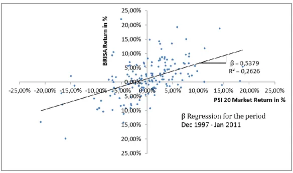
The CAPM measures the variance of the returns, systematic risk for a well-diversified portfolio, through a variable beta which determines the sensitivity between the returns of an asset with the variations of the market portfolio. Beta is estimated by the slope of the regression between the returns of stock i with market returns and is given as follows:
(1) 𝑅̅𝑖 = 𝑎 + 𝑏𝑅̅𝑚
If we take this regression, as an example, for the case of Brisa – Auto-Estradas
de Portugal on PSI20 market returns, we observe a Beta of 0.5379, which
means that Brisa stock returns are less volatile than the market in nearly 50%. This means that an upward movement in the market of 1% will theoretically move Brisa stock up by 0.5379%.
Figure 1. Brisa Beta Regression for the period Dec 1997 - Jan 2011
Additionally, the model considers two other components, the first is the existence of a risk-free asset, which can be defined as an asset that has no default risk (Damodaran, 2004), typically issued by a government seen as default free and that ensures no uncertainty about the reinvestment rates in the investment time horizon. Bruner et al. (1998) conducted a survey to corporations, financial advisers and academic textbooks and found that there was a strong preference to use long term bonds as yields, mainly 10 and 30 years as the riskless rate.
Secondly, the market risk premium (MRP) is measured by the difference between the expected return of the market and the risk-free rate. Damodaran (2004) defines it as the extra return that would be demanded by investors for shifting their money from a riskless investment to an average risk investment. Campbell (2007) states that the equity premium is not a constant number and must be estimated in each point in time, meaning that there is no consensus on which value it should assume. Fama & French (2002) suggest a historical MRP of 5.57% for the stocks of the S&P 500 in the period between 1872 and 2000 Fernandez et al. (2014) conducted a survey that collected information on the MRP used by companies, finance professors and financial analysts in Portugal during the years 2011 to 2014, where they observed values from 6.1% to 8.5%. Aswath Damodaran, in his online archive (updated 1st January 2015), considers a historical arithmetic average MRP over 10 year US treasury bonds, for the period of 1928 to 2014, of 6.25%. Dimson et al (2011) suggest a geometric average and arithmetic average worldwide equity premium, for the period between 1900 and 2010, of 3.8% and 5.0% respectively. Ibbotson (2011)
suggests a 5.5% historical geometric average MRP and 5.9% for the arithmetic average, for the period between 1926 and 2010. Many other authors have contributed to this discussion, in this paper we will assume the MRP to be a constant 6%.
The CAPM equation for the expected return of an asset i (or the cost of equity on an investment i) is given as:
(2) 𝑅̅𝑖 = 𝑅𝐹+ 𝛽𝑖 (𝑅̅𝑀− 𝑅𝐹)
where
𝑅𝐹 is the risk-free interest rate;
𝛽𝑖 is the exposure to risk of stock i to the market;
𝑅̅𝑀 is the market expected return.
The assumptions discussed previously are subject to strong criticism in the literature, since these conditions are not verified in practice. Despite this fact, due to its simplicity and ease of use, the CAPM is one of the most used models for evaluating returns and portfolio performance or estimating the cost of capital. To attest the validity of the model when evaluating capital projects, Welch (2008) asked professors if they recommended the CAPM for estimating the cost of capital and 75% answered positively. Bruner et al. (1998), in their aforementioned survey, also found that the CAPM is the dominant method for estimating the cost of capital.
2.3. Discount Rate used in PPP’s
The discount rate is used in financial valuation to account for time value of money (TVM). Damodaran (2004) defines TVM by stating that one Euro today is more valuable than one Euro in the future because we can invest that Euro and get a positive return on it. The discount rate is used to discount projects future cash flows to present terms, in this sense.
Sarmento (2010) states that the PSC is assessed over the PPP project life span in NPV terms, which means that the rate used to discount cash flows provides a huge impact to project analysis.
The same author concludes that there are 5 main approaches regarding PPP discount rates and they are presented as follows:
1) The discount rate should reflect government policy preferences, using a ‘social rate of time preferences’. Grimsey & Lewis (2005) divide the concept in two elements: the first is the basic ‘social time preference rate’ (STPR), which represents the rate that society is willing to receive now rather than in the future. HM Treasury (2003) Green Book suggests that for developed countries, this value is between 3.5% and 4.0% in real terms (before allowing for price inflation). The second part of the concept is to consider other factors, to ensure that the public sector does not assess the benefit of projects without taking into account the risk that it exposes taxpayers to;
2) The discount rate should reflect the ‘social opportunity cost of capital’ (SOCC), mainly used in Canada and New Zealand. Corresponds to the
pre-tax internal rate of return (IRR) that can be expected from private sector investments with the same risk. It is in fact calculated using a derivation of the CAPM;
3) The discount rate is a mix between the STPR and SOCC, the appropriate discount rate is the sum of the tax-exclusive real interest cost of government debt, the marginal income tax paid to private sector capital and systematic risk;
4) ‘Equity premium’, when the cost of capital is below the CAPM estimated values the discount rate should correspond to the pre-tax government borrowing rates;
5) The discount rate corresponds to the risk-free rate of the country, in other words, the interest rate of public debt for the project longevity.
In 2003, Portugal established the discount rate for the PSC in the law. It is composed by the inflation rate and the real nominal discount rate, which are combined using the Fisher equation (Cruz & Marques, 2013):
(3) Nominal Discount rate = [(1 + real discount rate) x (1 + inflation rate)] – 1
The real nominal discount rate was determined to be 4.0% by the Ministry of Finance in 2003 (Cruz & Marques, 2013).
Australia is an example of a country that adopted a different model to obtain appropriate discount rates, based on the CAPM. The Victoria Department of Treasury and Finance (2003) made a report accounting the use of discount rates in the Partnerships Victoria process where this topic is explored. The calculation of the discount rate was based on the different risks faced by each
project. Three groups of risk bands were defined: ‘Very Low’, ‘Low’ and ‘Medium’, attributing asset betas up to 0.3, 0.5 and 0.9 respectively. The risk-free rate considered was assumed to be the yield of Commonwealth Bonds with a 10 year maturity. The risk premium considered was 6.0%. Here we will propose the use of the CAPM for Portuguese road sector PPPs, assuming the same risk premium.
Cruz & Marques (2013) argue that from the public sector’s perspective the discount rate used is generally the ‘risk-free rate’, that is, the rate on long term government bonds. They add that the private sector should discount cash flows using a Weighted Average Cost of Capital (WACC) measure. They finally refer to an ongoing debate in the literature, regarding whether the same discount rate should be used for PSC and PPP bids. Grout (2003) argues that public sector discount rates should be lower than for the private sector, if not that would indicate that private provision was less efficient than public, since present values in the first case will be overestimated.
The discount rate has a huge influence in the choice the government makes: higher discount rates will favor the PPP option, because payments from the government to the private sector are mostly scheduled for the medium to long term, therefore devaluating payments and making the PPP option look ‘cheaper’. On the other hand, under traditional procurement a large portion of the expenditure is made in the first years, during the construction phase, therefore when discounting those payments, they will be less devaluated than those occurring in a distant future (Cruz e Marques, 2013).
3. Methodology & Data
Our goal is to calculate the appropriate discount rate for Portuguese PPPs in the road sector using the CAPM. In this section we describe the approaches used to calculate the private discount rate.
Our dataset is composed of 20 road sector Portuguese PPPs, described in the following table by project, contract data, contract length and contract term.
[Insert Table I here]
As described in chapter 2.2, we need three factors to calculate the equity cost of capital (𝑟𝐸) for a project. They are the risk-free rate (𝑅𝐹), a factor beta (𝛽𝑖 ) and the MRP, which is the difference between market return (𝑅̅𝑀) and 𝑅𝐹. In the following subsections, each element of the model is explained. Afterwards, we introduce the WACC specification and the regression method.
3.1. Risk-free rate
The risk-free rate is considered to be the European benchmark of 10 years German Bunds yields. At the time of each PPP contract we collected data on the yields based on the Bloomberg database. We also add to our database the spreads between the referred Bund yields and Portuguese Treasury Bonds (OT) 10 years at the same date. In section 3.5, we use the latter spread as a variable to observe if it has an impact on the cost of debt.
3.2. Beta
use comparable firms in the same industry and compute an average beta for the sector, another is the use of an asset beta as in the Australian case of Partnerships Victoria, discussed previously. We opted for the first method, since an asset beta is determined by assuming that the government is undertaking the project and retains all systematic risks, while here we are considering a private perspective. We used Thomson Reuters’ Datastream to collect monthly data on stocks’ quotes, dividends and market quotes on five European companies from four different markets, from 1995 onwards until the month after the date of the last PPP contracted in 2010 (Pinhal Interior). The comparables used were the following concessionaire firms.
[Insert Table II here]
As discussed in Section 2.2, we first compute stock returns and market returns1 and then execute a slope regression using both, to obtain a beta for each firm. We used the following formulas to compute the returns:
(4) 𝑅̅
𝑖,𝑗 =
𝑃𝑟𝑖𝑐𝑒𝑖,𝑗− 𝑃𝑟𝑖𝑐𝑒𝑖,𝑗−1+ 𝐷𝑖𝑣𝑖𝑑𝑒𝑛𝑑𝑠𝑗 𝑃𝑟𝑖𝑐𝑒𝑖,𝑗−1
where,
𝑅̅𝑖,𝑗 are the returns of stock i in month j
𝑃𝑟𝑖𝑐𝑒𝑖,𝑗 is the price of stock i at the end of month j
𝐷𝑖𝑣𝑖𝑑𝑒𝑛𝑑𝑠𝑗 are the dividends on stock i in month j
(5) 𝑅 ̅ 𝑀𝑎𝑟𝑘𝑒𝑡
𝑖,𝑗=
𝐼𝑛𝑑𝑒𝑥𝑖,𝑗 − 𝐼𝑛𝑑𝑒𝑥𝑖,𝑗−1+ 𝐷𝑖𝑣𝑖𝑑𝑒𝑛𝑑𝑠𝑗
𝐼𝑛𝑑𝑒𝑥𝑖,𝑗−1
where,
𝑅 ̅ 𝑀𝑎𝑟𝑘𝑒𝑡𝑗 is the return of market i in month j
𝐼𝑛𝑑𝑒𝑥𝑖,𝑗 is the index i quote at the end of month j
𝐷𝑖𝑣𝑖𝑑𝑒𝑛𝑑𝑠𝑗 are the dividends paid on the index in month j
Beta unlevered (𝛽𝑢) is the beta of a firm without any debt, it takes away the financial benefit of holding debt in the capital structure of the firm.
In order to obtain a 𝛽𝑢 for each PPP, firstly, we computed the returns of each comparable firm and index from three years before the date of the contract of each PPP project. Secondly, we computed the slope between each of the comparable firms and index returns, obtaining a beta for each. Finally, we calculated an average of the comparable firms’ betas for each project.
Since PPPs are highly leveraged companies that, as discussed in section 2.1, use leverage levels of 70% to 90%, we have to adjust betas for the leverage in each PPP. We use the following formula (as per Damodaran, 2004):
(6) 𝛽
𝑙= 𝛽𝑢[1 + (1 − 𝑡) (
𝐷 𝐸)] where,
𝛽𝑙 is the levered beta for the equity in the firm
𝛽𝑢 is the unlevered beta of the firm
𝐷
𝐸 is the Debt/Equity Ratio of the Firm
Corporate tax rate is considered to be the corporate tax rate currently in force in Portugal, 25%. As for the D/E ratio, leverage levels for each PPP are collected from Sarmento & Renneboog (2014b).
Additionally, we obtained from Damodaran Online unlevered betas for the European transportation sector, in the years 2011, 2012 and 2013 and computed the average of these values. A beta unlevered value of 0.57 was obtained and we then applied the same methodology as before, computing new levered betas to compare with our own calculations.
3.3. Market Risk Premium
As discussed in Section 2.2, the MRP is not a constant number. In the examples given, we observe values which range between 5% and 6.25%. Here, we will follow the assumption of a 6% MRP, as was done in the case of the Australian Victoria Partnerships (2003).
3.4. WACC
To account for the benefits that leverage brings to an investment and since PPPs are highly leveraged firms, we should consider a discount rate that considers those benefits, including the interest tax shield. This can be done using a WACC methodology. The WACC is given by the following formula: (7) 𝑟𝑤𝑎𝑐𝑐 = 𝐸 𝐸 + 𝐷𝑟𝐸+ 𝐷 𝐸 + 𝐷𝑟𝐷(1 − 𝑡) where,
E is the market value of equity of the firm D is the market value of debt of the firm
𝑟𝐸 is the equity cost of capital
𝑟𝐷 is the debt cost of capital
t is corporate tax rate
In the previous section, we proposed a formula to compute 𝑟𝐸 for a firm, now, in
order to apply equation 7, we will need a method to calculate 𝑟𝐷, the cost of
debt, which measures the borrowing cost for the firm. The cost of debt equation is given as:
(8) 𝑟𝐷 = 𝐸𝑢𝑟𝑖𝑏𝑜𝑟 + 𝑃𝑟𝑜𝑗𝑒𝑐𝑡𝑆𝑝𝑟𝑒𝑎𝑑
6-month Euribor rates (annual average at the date of each contract) are collected from Bloomberg. Data for project spreads is collected from Sarmento & Renneboog (2014b) and regards the bank spreads of each PPP.
3.5. Regression Method
We began to explain the methodology by introducing the calculation of the appropriate discount rates. Now, we will test the relationship of model betas, cost of debt and the cost of equity with three independent variables. Firstly, in this section we address all the variables in our methodology. Secondly, we present the used regressions and then finish by reporting descriptive statistics for all the variables and correlation matrix of the regressions.
Calculation of the cost of equity was defined above using two different methodologies. We first describe the equation for the comparable firms method and its composing variables.
(9) 𝑟𝐸 = 𝑅𝐹+ 𝛽𝐿 (𝑅̅𝑀− 𝑅𝐹)
where,
𝑟𝐸 is the cost of equity obtained for each PPP contract using the comparable
firms methodology;
𝑅𝐹 stands for the risk-free rate (10 year German Bund yields) at the date of each contract, collected from Bloomberg;
𝛽𝐿 is the beta leverage calculated for each PPP using the comparable firms methodology, calculated based on the computed beta unlevered average of five different firms that operate highway concessions and on the level of D/E in the capital structure of each PPP (collected from Sarmento & Renneboog, 2014b). The next two variables are used in equation 6 which allows to compute the beta leverage:
𝛽𝑈 stands for the beta unlevered calculated for each PPP using the comparable firms methodology;
Lev represents the percentage level of debt in the capital structure of each PPP,
taken from Sarmento & Renneboog (2014b);
Rm stands for the market return, assumed to be constant at 6% above the
risk-free rate.
For the second method, using Damodaran Online data, we apply a similar formula:
(10) 𝑟𝐸𝐷 = 𝑅𝐹 + 𝛽𝐿𝐷(𝑅̅𝑀 − 𝑅𝐹) where,
𝑟𝐸𝐷 is the cost of equity for each PPP contract, calculated using the values
provided from Damodaran Online;
𝛽𝑈𝐷 is the beta unlevered average obtained using the values provided by Damodaran Online;
𝛽𝐿𝐷 is the beta levered calculated for each PPP using the values provided by
Damodaran Online. The method for its calculation is given again by equation 6, but using the average beta unlevered for European transportation sector firms in the years 2011, 2012 and 2013 and again the variable Lev.
The remaining variables refer to the computation of the WACC using the two different cost of equity discount rates, as in equation 7. They are summarized below:
t is the Portuguese corporate tax rate, that is assumed to be 25%;
𝑟𝐷 represents the cost of debt of each PPP contract and is calculated as in equation 8;
𝑊𝐴𝐶𝐶 stands for the weighted average cost of capital for each PPP using the cost of equity from the comparable firms method as a factor in the WACC model;
𝑊𝐴𝐶𝐶𝐷 stands for the weighted average cost of capital for each PPP using the
cost of equity from the sector average method, as a factor of the WACC model. In the following tests, we will use as dependent variables the already introduced 𝛽𝐿, 𝛽𝐿𝐷, 𝑟𝐷,𝑟𝐸 and 𝑟𝐸𝐷. We will now explain the independent variables in our
OLS regressions, as well as their expected influence over the dependent variables in our model. The three independent variables are listed below.
𝑆𝑝𝑟𝑒𝑎𝑑, the value of 10 year Portuguese Treasury bond spread at the date of each contract in regards to the benchmark 𝑅𝐹. We expect that the cost of debt should not be very influenced by this variable since its values are not very high. Nevertheless, the cost of debt should be higher since the rates of Portuguese Treasury bonds are higher than German Bunds’.
𝐹𝑜𝑟𝑒𝑖𝑔𝑛𝑆ℎ𝑎𝑟𝑒ℎ𝑜𝑙𝑑𝑒𝑟𝑠 is a dummy variable with the value of 1 if the majority of a project’s equity capital is owned by foreign shareholders and 0 if the majority of equity capital is owned by domestic (Portuguese) shareholders. It is expected that a majority of foreign capital should be associated with lower costs of financing, since foreign shareholders should have access to more markets and
inspire more confidence in international markets (namely, with better credit ratings).
𝑃𝑎𝑦𝑚𝑒𝑛𝑡 is a dummy variable with the value of 0 if the payment is due by a toll concession and 1 if it is based on an availability scheme. In an availability scheme the government is made to pay a fixed rent, as long as the asset is in the conditions specified in the contract. This type of payment allocates demand risk (the risk that traffic volume is below projected) to the public entity. Therefore, uncertainty regarding long-term revenues for the private party is lower, which is expected to reduce the cost of capital and the cost of financing the project.
The first regressions’ objective is to assess if there is a causality relationship between the independent variables Shareholders and Payment and the level of leverage implied in levered betas, computed using our two methodologies: (11) 𝛽𝐿 = 𝛼0+ 𝛼1𝐹𝑜𝑟𝑒𝑖𝑔𝑛𝑆ℎ𝑎𝑟𝑒ℎ𝑜𝑙𝑑𝑒𝑟𝑠 + 𝛼2𝑃𝑎𝑦𝑚𝑒𝑛𝑡 + 𝜀 (12) 𝛽𝐿𝐷 = 𝛿0+ 𝛿1𝐹𝑜𝑟𝑒𝑖𝑔𝑛𝑆ℎ𝑎𝑟𝑒ℎ𝑜𝑙𝑑𝑒𝑟𝑠 + 𝛿2𝑃𝑎𝑦𝑚𝑒𝑛𝑡 + 𝜀
The second regression’s purpose is to test whether these independent variables, adding this time the Spread variable as well, affect the cost of financing the PPP scheme reflected in the cost of debt (𝑟𝐷):
(13) 𝑟𝐷 = 𝛾0+ 𝛾1𝐹𝑜𝑟𝑒𝑖𝑔𝑛𝑆ℎ𝑎𝑟𝑒ℎ𝑜𝑙𝑑𝑒𝑟𝑠 + 𝛾2𝑃𝑎𝑦𝑚𝑒𝑛𝑡 + 𝛾3𝑆𝑝𝑟𝑒𝑎𝑑 + 𝜀
The final regressions intend to evaluate the relationship of independent variables Shareholders and Payment with the cost of equity (𝑟𝐸) of the PPP, that is, whether the cost of equity of a PPP is affected by its shareholder structure
(14) 𝑟𝐸 = 𝜃0+ 𝜃1𝐹𝑜𝑟𝑒𝑖𝑔𝑛𝑆ℎ𝑎𝑟𝑒ℎ𝑜𝑙𝑑𝑒𝑟𝑠 + 𝜃2𝑃𝑎𝑦𝑚𝑒𝑛𝑡 + 𝜀 (15) 𝑟𝐸𝐷 = 𝜌0+ 𝜌1𝐹𝑜𝑟𝑒𝑖𝑔𝑛𝑆ℎ𝑎𝑟𝑒ℎ𝑜𝑙𝑑𝑒𝑟𝑠 + 𝜌2𝑃𝑎𝑦𝑚𝑒𝑛𝑡 + 𝜀
Descriptive statistics and correlation matrix of these variables are presented in the next tables. Breusch-Pagan and White tests were conducted to test for the presence of heteroscedasticity, which was not found. Observation of the correlation matrix shows no signs of multicollinearity.
4. The Portuguese PPP experience
Portugal has had some experiences with the private provision of public services, through concession deals, since the 70s. In the mid-90s the financial close on the Vasco da Gama bridge concession contract (Lusoponte) lead to the beginning of the PPP movement in Portugal (European PPP Expertise Center (EPEC), 2014). As will be shown, this was mostly related to road sector investments, which this work focuses on. There was, however, also an important use of the PPP model in the health sector.
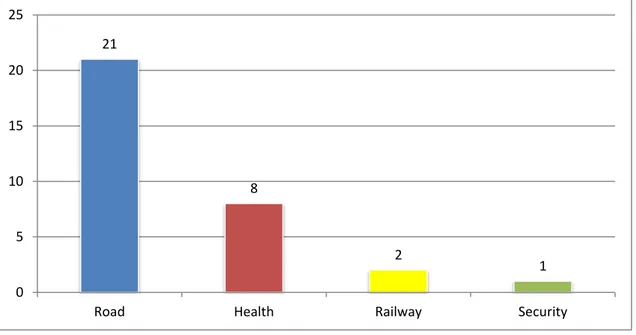
More specifically, as of 2015, according to Unidade Técnica de
Acompanhamento de Projetos2 (UTAP) (2015), there are 32 PPPs currently
operating in Portugal with the following sectorial distribution.
Figure 2. Portuguese PPP Projects Sectorial Distribution
Source: Adapted from UTAP (2015), p.11
21 8 2 1 0 5 10 15 20 25
EPEC (2014) separates the PPP movement in road sector public investments in Portugal into two waves. The first wave was launched in the period between 1999 and 2006, with three real toll motorways and seven shadow toll motorways, (famously termed SCUTs - Sem Cobrança ao Utilizador - i.e. with no charges to users). The second wave, occurring between 2007 and 2010, consisted of seven road PPP schemes with a mix between real tolls and availability payments covering around 2000 km. It is also important to add that in 2010 and 2011 some PPP contracts were renegotiated by the government to lighten public expenditure in these contracts. One of the most significant changes was the availability scheme model introduced in the so-called SCUTs. It is therefore important to summarize the different types of road sector concessions and PPPs existing in Portugal. According to Direção Geral do
Tesouro e Finanças (2012) and UTAP (2015), these projects are subdivided
into three schemes:
Traditional concession with real tolls: where the private partner charges a toll on the direct user, not receiving any current payment by the State. This is the case of Brisa, Oeste, Lusoponte, Litoral Centro and Douro
Litoral.
Availability-payment concession: The state pays a certain amount to the private partner depending on road availability and, in return, receives toll payments collected by the private concessioner.
This is the case of former ‘SCUT’ concessions of Grande Porto, Norte
Algarve and Norte e Grande Lisboa (the latter was in fact, until 2010, a
traditional concession rather than a PPP).
Subconcessions and Tunel do Marão3: The state receives toll payments in the cases of motorways and pays the private sector a fee based on road and service availability, which is indexed to traffic.
This is the case of Pinhal Interior, Litoral Oeste, Douro Interior, Baixo
Tejo, Baixo Alentejo, Transmontana and Algarve Litoral.
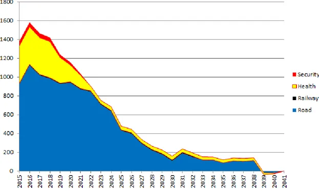
After an overview of PPPs existing in Portugal and their history, we now analyse the amount invested so far under this model, and how it affected public finances. UTAP (2015) states that the overall investment by private partners in the period from 1998 to 2014 reached 14,364 million euros. 93% of this expenditure pertains to road sector investments. As for future expenditures of the Portuguese government due to PPP contracts, we observe in the Government Budget for 2015 (Ministério das Finanças, 2014) an immediate high level of yearly payments above one billion euros until 2021, with significant, decreasing yearly amounts continuing until 2041, a significant burden to current and future Portuguese taxpayers. A graphical analysis on how payments are projected until 2041 is shown below.
Figure 3. Forecast of the annual evolution of payments to PPPs in m€
Source: Adapted from UTAP (2015), p.45
Now we take an overview of the most relevant merits and issues that have been described in different sources, regarding the use of PPPs in Portugal.
Marques & Silva (2008) summarize the benefits of road sector PPPs in Portugal: they argue that the conclusion of the national motorway network was anticipated with great execution capacity by both parties leading to an economic boost, the management of the network was ensured for an extended period, there was a transfer of a great part of risks to the private sector, Portuguese companies involved in the PPP schemes faced new challenges and improved competences and finally the reduction of road accidents.
In opposition, the high usage of PPPs in Portugal has been heavily criticized, as public authorities, when undertaking these projects, seemed at times to be more
concerned about meeting European rules concerning budget deficits, than with value for money. Sarmento (2010) raised the issue, the decision to deliver public investment through PPPs is related to an ‘’off budget temptation’’ as opposed to being based on efficient public procurement procedures.
Sarmento & Reis (2013) report that future payments due by the Portuguese government to honor these contracts represent an annual effort above 0.5% of GDP until almost 2030, while between 2014 and 2020 these payments will rise up to 1%. They also observe that Portugal is the European PPP leader when considering capital expenditure as a percentage of GDP, with a figure of more than 10%, according to the European Investment Bank.
Marques & Silva (2008) conclude that the existing problems in road concessions had three kinds of consequences for the Portuguese state: ex post financial renegotiations which created additional payments; ill-conceived contracts; weak control and inspection of the concessions. These problems were rooted in the absence of adequate environmental evaluation, political issues, poor management of expropriations, weak technical preparation, an ineffective learning process and an inefficiently organized public administration.
5. Results
In this section, we start by presenting discount rates obtained for each PPP and afterwards we discuss the results of the regressions.
The calculated discount rates for the cost of equity seem to be very high. To fully understand this phenomenon, we need to split the CAPM cost of equity formula (equation 9) into two components. The first is composed of the risk-free rate and the market risk premium. Both are collected from market data, irrelevant to the financial structure of the firm. The second includes levered betas, computed using equation 6. The last equation can be subdivided into three variables: unlevered beta, which is computed according to market data, using data for 5 listed firms and the European transportation sector average, but varies due to each project contract data in the case of the comparable firms method; the tax rate, collected from external sources, has no impact in the different projects; finally, the Debt to Equity ratio, that varies across each PPP, as it depends on the different financial structure of each project.
The high leverage levels showed by each PPP, normally ranging between 70 to 90%, seem to be the critical factors influencing higher or lower levered betas leading to a higher or lower cost of equity, respectively. To illustrate, we show our sample’s highest and lower cost of equity projects and try to explain these deviations in relation to other projects.
[Insert Table V here]
In the case of the projects with higher costs of equity, we observe that leverage levels over 90% lead to massive discount rates. When looking at the projects
with the lower three CAPM discount rates, we find two opposing cases. The first is the Algarve Litoral project, its 11% cost of equity is very low compared to other projects due to the low leverage of its capital structure. One explanation for this fact could be that this project was contracted during the peak of the subprime financial crisis, a time associated with a strong “credit crunch”. The case of Grande Porto and Norte Litoral have a contrasting explanation for their lower unlevered beta average values, which ultimately result from the markedly lower betas of comparable firms in the years 2001 and 2002.
The introduction of the WACC methodology to obtain discount rates allows to consider the actual capital structure of the PPP and also to consider tax savings due to the use of debt. Since project risk is small and insured by the intervention of the government, it allows for low debt interest rates, meaning that PPP profitability will benefit from the highly levered capital structure. We find that the WACCs computed are all under 9%, a fairly high level even for a capital intensive project like a PPP. We conclude that the appropriate discount rates for PPPs for the private sector are between 6 to 8%. Additionally, we find that using the sector average method, discount rates are normally lower than in the comparables methodology, due to lower unlevered betas, in most cases.
[Insert Table VI here]
The discount rates presented above were subject to tests on its components and on the cost of equity. We start by analyzing if the presence of foreign shareholders in the PPP and whether the government payments are performed under an availability scheme affect the risk implied in computed levered betas.
[Insert Table VII here]
As predicted, we observe negative coefficients for the ForeignShareholders and
Payment variables. Thus, we find that if the majority of equity capital in the PPP
is constituted by foreign shareholders, project risk seems lower, at the 10% significance level. On the other hand, even though the coefficient is negative, in line with our theoretical prediction, we could not find statistical significance regarding the influence of the payment method. We observe the same type of behavior for levered betas obtained using both methodologies.
In our second test we aimed to test the relationship of the aforementioned variables, along with the Spread variable, with the cost of debt. We could not find a statistically significant relationship with any of the variables. Despite this fact, it comes as a surprise that ForeignShareholders has a positive coefficient, whereas we expected a majority of foreign shareholders should be associated with a decrease of the cost of debt. The other surprise is that the Spread has no explanatory power whatsoever, while even though bond yield spreads are generally low throughout the considered period, they were expected to raise marginally the cost of debt. As we expected, the coefficient for the Payment variable is negative.
[Insert Table VIII here]
The final regressions consider again the same variables, ForeignShareholders and Payment. Its objective is to test if a majority of foreign shareholders is associated with lower costs of equity and if the availability payment scheme is linked to lower discount rates. We observe negative coefficients in the case of
both variables, as expected. It is interesting that, once again, only the influence of the ForeignShareholders dummy seems to be statistically significant at a 10% level. Its coefficient values are high enough to, on average, be associated with a decrease of the cost of equity by nearly half.
6. Conclusion
In this study, we addressed a method to compute discount rates for PPPs from the private sector perspective. As such, we computed discount rates based on the CAPM and WACC models for 20 Portuguese PPPs in the road sector, using two different methodologies to derive beta values.
In one case, we find that when considering European transportation sector average betas, the calculated discount rates are in the majority of the cases lower than in the second case, where betas are obtained from a set of comparable firms.
Moreover, we argue that the CAPM has important limitations when considering PPPs since it is excessively affected by projects’ highly leveraged capital structure. Due to this fact, rates obtained with the CAPM reach very high levels. Also, we verified that having a majority of foreign shareholders in the PPP’s capital structure seems to negatively affect, at the statistically significant level of 10%, levered betas and the cost of equity as a discount rate. Government bond yield spreads and the type of payment method from the government (with or without an availability scheme) showed no statistically significant relationship with the cost of debt, levered betas or the cost of equity.
The proposed methodology could be used in other PPP projects that present different capital structures and share the same set of sectorial comparable firms. Future works can also add more firms, to better model betas in a sectorial perspective. More variables could also be included in econometric tests, to address their influence over discount rates. It should be added that there are
different forms of addressing the discount rate problem and, while our method allows to pinpoint adequate rates for Portuguese road PPP projects in general, it does not attempt to obtain rates for specific projects, which would require a consideration of all sources of specific risk for each PPP.
References
Bruner, R., Eades, K., Harris, R. & Higgins, R. (1998). Best Practices in Estimating the Cost of Capital: Survey and Synthesis. Financial Management 27, 13-28.
Campbell, J. (2007). Viewpoint: Estimating the Equity Premium. Canadian Journal of Economics Vol.41. 1-21.
Corner, D. (2006). The United Kingdom Private Finance Initiative: The Challenge of Allocating Risk. OECD Journal on Budgeting Vol.5/3. 37-55. Cruz, C. & Marques, R. (2013). Infrastructure Public-private Partnerships:
Decision, Management and Development. Berlin: Springer.
Damodaran, A. (2004). Corporate Finance: Theory and Practice, 2nd Ed. USA: Wiley.
Damodaran, A. (2015). Damodaran Online [Online]. Available from: http://pages.stern.nyu.edu/~adamodar/New_Home_Page/datafile/histret SP.html [Accessed: 31/07/2015].
Dimson, E., Marsh, P. & Staunton, M. (2011). Equity Premiums Around the World. CFA Institute.
Direcção Geral de Tesouro e Finanças (2012). Relatório de 2012 Parcerias Público Privadas e Concessões. Ministério das Finanças.
Elton, E., Gruber, M., Brown, S. & Goetzmann, W. (2011). Modern Portfolio Theory and Investment Analysis, 8th Ed. Asia: Wiley.
European PPP Expertise Center (2014). Portugal: PPP Units and Institutional Framework, Luxemburg.
Fama, E. & French, K. (2002). The Equity Premium. Journal of Finance Vol.57 No.2. 637-659.
Fernandez, P., Linares, P. & Acín, I. (2014). Market Risk Premium Used in 88 Countries in 2014: A Survey with 8228 Answers. IESE Business School.
Grimsey, D. & Lewis, M. (2002). Evaluating the Risks of Public Private Partnerships for Infrastructure Projects. International Journal of Project Management 20. 107-118.
Grimsey, D. & Lewis, M. (2004). Public Private Partnerships: The Worldwide Revolution in Infrastructure Provision and Project Finance. Cheltenham, UK and Northampton, Mass.: Edward Elgar.
Grimsey, D. & Lewis, M. (2005). Value-for-Money Measurement in Public-Private Partnerships. EIB Papers 10 (2). 32-56.
Grout, P. (2003). Public and Private Sector Discount Rates In Public-Private Partnerships. The Economic Journal 113. 62-68.
Hemming, R. (2006). Public-Private Partnerships, Government Guarantees, and Fiscal Risk, Washington DC: International Monetary Fund.
HM Treasury (2003). The Green Book: Appraisal and Evaluation in Central Government, The Stationery Office, London.
International Monetary Fund (2004). Public-Private Partnerships [Online]. Available_from:_http://www.imf.org/external/np/fad/2004/pifp/eng/031204 .htm [Acessed: 1/7/2015].
Lintner, J. (1965). The Valuation of Risk Assets and the Selection of Risky Investments in Stock Portfolios and Capital Budgets. Review of Economics and Statistics. 47, 13-37.
Markowitz, H. (1952). Portfolio Selection. Journal of Finance. 7, 77-91.
Marques, R. & Silva, D. (2008). As Parcerias Público-Privadas em Portugal. Lições e Recomendações. Revista de Estudos Politécnicos Vol. VI (10), 33-55.
Ministério das Finanças (2014). Orçamento de Estado para 2015, Lisboa
Morallos, D. & Amekudzi, A. (2008). The State of the Practice of Value for Money Analysis in Comparing Public Private Partnerships to Traditional Procurements. Public Works Management & Policy Vol.13 (3), 114-125. Mossin, J. (1966). Equilibrium in a Capital Asset Market. Econometrica. 34,
768-783.
Organization for Economic Co-Operation and Development (2008). Public-Private Partnerships: In Pursuit of Risk Sharing and Value for Money. OECD Publishing.
Sarmento, J. (2010). Do Public-Private Partnerships Create Value for Money for the Public Sector? The Portuguese Experience. OECD Journal on Budgeting Vol.2010/1.
Sarmento, J. (2013). Parcerias Público-Privadas. Fundação Francisco Manuel dos Santos. Portugal: Relógio D’Água Editores.
Sarmento, J. & Renneboog, L. (2014a). Public-Private Partnerships: Risk Allocation and Value for Money. CentER Discussion Paper Vol. 2014-022.
Sarmento, J. & Renneboog, L. (2014b). The Portuguese Experience with Publi-Private Partnerships. CentER Discussion Paper Vol. 2014-005.
Sarmento, J. & Reis, R. (2013). Buy Back PPPs: An Arbitrage Opportunity. OECD Journal on Budgeting Vol.12/3.
Sharpe, W. (1964). Capital Asset Prices: A Theory of Market Equilibrium under Conditions of Risk. Journal of Finance. 19, 425-442.
Unidade Técnica de Acompanhamento de Projectos (2015).Boletim Trimestral PPP – 1º Trimestre de 2015, Ministério das Finanças, Lisboa.
Victoria Department of Treasury and Finance (2003). Partnerships Victoria: Use of Discount Rates in the Partnerships Victoria Process, Technical Note, July, Victoria, Australia.
Welch, I. (2008). The Consensus Estimate for the Equity Premium. Academic Financial Economists in December 2007, Unpublished Working Paper. Brown University.
Yescombe, E. (2007). Public-Private Partnerships: Principles of Policy and Finance, 1st Ed. UK: Elsevier.
Appendix Table I.
PPP Road Sector Dataset
A description of all Portuguese road sector PPP projects considered in this study is given in this table. This includes projects’ name, contract start date, contract length and year of contract term.
Source: Own table and UTAP (2015)
PPP Project Contract Data Contract Length Contract Term
Algarve litoral 20-04-2009 30 2039 Algarve 11-05-2000 30 2030 Baixo Alentejo 30-01-2009 30 2039 Baixo Tejo 24-01-2009 30 2039 Beira Interior 13-09-1999 30 2029 BLA 28-04-2001 30 2031 Costa da Prata 19-05-2000 30 2030 Douro Interior 25-11-2008 30 2038 Douro Litoral 05-01-2007 27 2034 Grande Lisboa 10-01-2007 30 2037 Grande Porto 16-09-2002 30 2032 Interior Norte 30-12-2000 30 2030 Litoral Centro 30-09-2004 30 2034 Litoral Oeste 26-02-2009 30 2039 Norte Litoral 17-09-2001 30 2031 Norte 09-07-1999 36 2035 Oeste 05-01-1999 30 2029 Transmontana 09-12-2008 30 2038 Tunel Marão 30-05-2008 30 2038 Pinhal interior 28-04-2010 30 2040
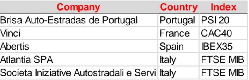
Table II.
Comparable Firms for Beta Calculation
In this table, we find the comparable listed European firms that operate in the road concession business, used for the computation of a European Beta unlevered average for each contract.
Source: Own table and DataStream Reuters
Company Country Index
Brisa Auto-Estradas de Portugal Portugal PSI 20
Vinci France CAC40
Abertis Spain IBEX35
Atlantia SPA Italy FTSE MIB
Table III.
Descriptive Statistics
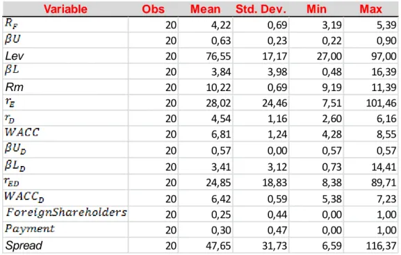
The following table represents the number of observations, mean, standard deviation, minimum value and maximum of each of the variables in this study. 𝑅𝐹 stands for the
risk-free rate, given in %; 𝛽𝑈 stands for the beta unlevered of the comparable firms methodology, given in units; Lev corresponds the % of debt in the capital structure of each PPP; 𝛽𝐿 corresponds to the beta leverage of the comparable firms methodology, given in units; Rm represents the market return, given in %; 𝑟𝐸 is the calculated CAPM cost of equity discount rate using the comparable firms methodology, given in %; 𝑟𝐷 represents the cost of debt of each contract, given in %; 𝑊𝐴𝐶𝐶 stands for the weighted average cost of capital using the comparable firms methodology, given in %; 𝛽𝑈𝐷 is the beta unlevered average using the values provided by Damodaran Online, given in units; 𝛽𝐿𝐷 is the beta levered calculated provided by the Damodaran Online methodology, given in units; 𝑟𝐸𝐷 is the calculated CAPM cost of equity discount rate using the Damodaran Online methodology, given in %; 𝑊𝐴𝐶𝐶𝐷 stands for the weighted
average cost of capital using the Damodaran Online methodology, given in %; 𝐹𝑜𝑟𝑒𝑖𝑔𝑛𝑆ℎ𝑎𝑟𝑒ℎ𝑜𝑙𝑑𝑒𝑟𝑠 is a dummy variable that is 1 if the majority of equity capital is owned by foreign shareholders and 0 if the majority of equity capital is owned by domestic (Portuguese) shareholders; 𝑃𝑎𝑦𝑚𝑒𝑛𝑡 represents a dummy variable that is 1 if the payment is due by a toll concession and 0 if it is based on an availability scheme; 𝑆𝑝𝑟𝑒𝑎𝑑 is the value of 10 year Portuguese Treasury bond spread (basis points) at the date of each contract in regards to the benchmark German bund 10 years risk-free rate.
Source: Own table
Variable Obs Mean Std. Dev. Min Max
20 4,22 0,69 3,19 5,39 20 0,63 0,23 0,22 0,90 Lev 20 76,55 17,17 27,00 97,00 20 3,84 3,98 0,48 16,39 Rm 20 10,22 0,69 9,19 11,39 20 28,02 24,46 7,51 101,46 20 4,54 1,16 2,60 6,16 20 6,81 1,24 4,28 8,55 20 0,57 0,00 0,57 0,57 20 3,41 3,12 0,73 14,41 20 24,85 18,83 8,38 89,71 20 6,42 0,59 5,38 7,23 20 0,25 0,44 0,00 1,00 20 0,30 0,47 0,00 1,00 Spread 20 47,65 31,73 6,59 116,37
Table IV.
Correlation Matrix
The correlation matrix between independent variables shows no evidence of strong correlations. Therefore multicollinearity is not likely to lead to estimation problems.
Source: Own table
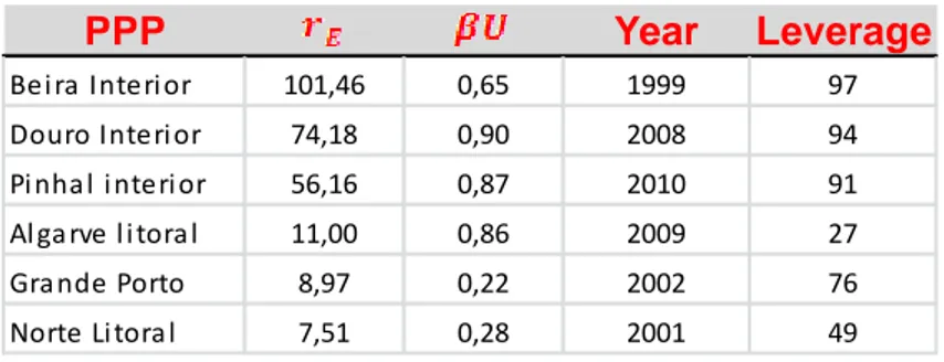
Table V.
Cost of Equity and the Effects of Beta Unlevered and Leverage
This table reports the highest and lowest cost of equity discount rates computed using the comparable firm methodology. Its purpose is to show the limitations of the CAPM in PPP projects regarding high leveraged capital structures and dependence on the beta factor of our comparable firm methodology.
Source: Own table Correlation Matrix 1 -0,378 1 0,3279 -0,3306 1 PPP Year Leverage Bei ra Interi or 101,46 0,65 1999 97 Douro Interi or 74,18 0,90 2008 94 Pi nha l i nteri or 56,16 0,87 2010 91 Al ga rve l i tora l 11,00 0,86 2009 27 Gra nde Porto 8,97 0,22 2002 76 Norte Li tora l 7,51 0,28 2001 49
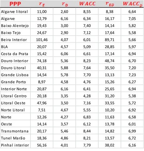
Table VI.
Discount rates
The following table describes computed discount rates for all 20 PPPs under study. The excessively high CAPM cost of equity values are explained by the high leverage of the PPP projects. The suggested preferred method to obtain discount rates for the private sector regarding PPPs is therefore the WACC. We find the majority of the WACCs computed to be between 6 to 8%, with some exceptions. We also find that both data methodologies yield similar rates, even though we observe, in most cases, lower values when using the European sector average as a benchmark.
Source: Own table PPP Al ga rve l i tora l 11,00 2,60 8,55 8,38 6,64 Al ga rve 12,79 6,16 6,34 16,17 7,05 Ba i xo Al entejo 19,43 3,00 7,40 14,14 5,82 Ba i xo Tejo 24,67 2,90 7,12 17,64 5,58 Bei ra Interi or 101,46 4,07 6,01 89,71 5,66 BLA 20,07 4,57 5,09 28,85 5,97 Cos ta da Pra ta 15,42 6,06 6,61 17,14 6,94 Douro Interi or 74,18 5,36 8,23 48,74 6,70 Douro Li tora l 40,31 5,88 7,64 35,50 7,20 Gra nde Li s boa 14,54 5,78 7,70 13,13 7,23 Gra nde Porto 8,97 4,58 4,76 15,26 6,27 Interi or Norte 20,87 6,16 6,41 25,65 6,94 Li tora l Centro 20,18 3,35 4,28 31,20 5,38 Li tora l Oes te 47,96 3,50 7,16 33,55 5,72 Norte Li tora l 7,51 4,67 5,55 10,20 6,92 Norte 12,26 4,27 6,83 11,63 6,58 Oes te 14,14 3,57 6,12 13,78 6,01 Tra ns monta na 20,17 5,46 8,44 14,82 6,99 Tunel Ma rã o 18,36 4,86 8,21 13,57 6,72 Pi nha l i nteri or 56,16 4,01 7,79 38,02 6,16
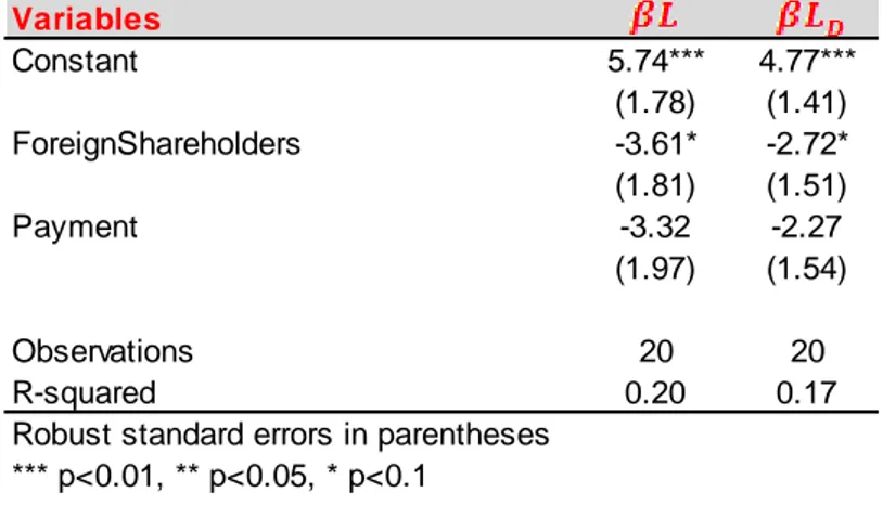
Table VII.
Levered Betas Regression
The dependent variables are Betas levered using the comparable firm methodology and the Beta levered using the European sector average. Both OLS tests include the described dummy independent variables, ForeignShareholders and Payment, in our methodology. We find statistical evidence at the 10% significance level of having a foreign majority shareholder position in the PPP to decrease levered Betas significantly in both cases.
Source: Own table
Table VIII.
Cost of Debt Regression
The dependent variable is projects’ cost of debt. OLS testing is performed, finding no evidence of statistically significant influence from any of our independent variables. Therefore, neither having a foreign shareholder majority in the PPP, nor the payment scheme or the spread of Portuguese bond yields seem to have an impact on the cost of debt of any of the projects.
Source: Own table Variables Constant 5.74*** 4.77*** (1.78) (1.41) ForeignShareholders -3.61* -2.72* (1.81) (1.51) Payment -3.32 -2.27 (1.97) (1.54) Observations 20 20 R-squared 0.20 0.17 Robust standard errors in parentheses
*** p<0.01, ** p<0.05, * p<0.1 Variables Constant 3.80*** (0.25) ForeignShareholders 0.23 (0.20) Payment -0.31 (0.23) Spread -0.00 (0.00) Observations 20 R-squared 0.24
Robust standard errors in parentheses *** p<0.01, ** p<0.05, * p<0.1