Calibration, Selection and Mosaicing of SMART-1 AMIE Images

Marco António Bernardino Raimundo Costa

Licenciado em Ciências da Engenharia Electrotécnica e de Computadores

Calibration, Selection and Mosaicing of

SMART-1 AMIE Images

Dissertação para obtenção do Grau de Mestre em Engenharia Electrotécnica e de Computadores

Orientador: José Manuel Fonseca, Professor Doutor,

FCT/UNL

Co-orientador: André Damas Mora, Professor Doutor,

FCT/UNL

Presidente: Prof. Doutor Yves Philippe Rybarczyk Arguente: Mestre Miguel Alexandre Dias Almeida

Vogais Prof. Doutor José Manuel Matos Ribeiro da Fonseca Prof. Doutor André Teixeira Bento Damas Mora

Calibration, selection and mosaicing of SMART-1 AMIE Images

Copyright © Marco António Bernardino Raimundo Costa, Universidade Nova de Lisboa

A

KNOWLEDGEMENTS

Queria começar por agradecer à minha família. Não seria nada sem a minha imparável avó e a sua energia eterna, capaz de fazer incríveis sacrifícios por aqueles que ama. Assim como o meu avô, pela qual a idade parece não passar e mantém o mesmo grande coração e boa disposição que sempre conheci. Não me podia esquecer da minha tia e as suas perguntas incessantes que me fazem sempre sorrir. E claro, à minha mãe com seu apoio constante e incentivo, mesmo nos momentos mais difíceis. Para terminar, ainda à sempre pequenina Maria Luís e da sua constante motivação para seguir em frente, sem a qual a escrita desta tese teria sido bastante mais complicada. És um sol com esse sorriso.

Queria também agradecer a todos os professores que nestes anos contribuíram para a minha aprendizagem, mas especialmente aos professores José Manuel Fonseca e André Mora. Foram como uns mentores neste último ano. A vossa incrível disponibilidade, interesse e rigor por tudo o que vos rodeia fez-me desejar encontrar mais pessoas como vós neste ciclo profissional que agora se inicia. Um sincero obrigado.

Durante estes muitos amigos e colegas deixaram a sua marca. Ao Luís Pedro pelas muitas horas a debater ideias e contribuição para este e muitos outros trabalhos. Ao Rui que nunca me deixou esquecer que continua a haver vida fora da faculdade. Ao Pedro pela constante boa disposição e good vibe. Ao Tiago pelo foco que imprime a tudo o que se envolve. A toda a Malta pela incessante conversa sobre filmes e séries que parece nunca irá parar. E a muitos outros que não disse o nome mas estão sempre presentes.

A

BSTRACT

Small Missions for Advanced Research in Technology (SMART-1), represented European Space Agency (ESA) first mission to the moon. It fulfilled the goal of improving the scientific knowledge of earth’s natural satellite, while testing new technologies that had never been used in space exploration. Among the on board instruments of SMART-1 was the Advanced Moon micro-Imager Experiment (AMIE). It was an imaging equipment whose mission was to map the lunar surface providing state-of-the-art resolution. Containing six filters inside its visual scope AMIE allowed the study of the surface composition by multispectral imaging.

This thesis aims at building a set of maps covering approximately all the Moon surface as it was mapped by the SMART-1 spacecraft, using the 31945 images captured by the AMIE instrument. During the Earth escape phase the instrument’s CCD was damaged by radiation, causing the accumulation of dark current and invalidating the laboratorial image calibration algorithm. The acquired dataset also suffered from scattered light that got beneath the CCD filters and reduced their contrast. In order to overcome this problem, a new calibration procedure was developed using the in-flight collected data and theoretical models, as well as a method to compensate for the reduced contrast in the filters.

For building the lunar maps, the images were individually analysed and classified accordingly to their visual quality and grouped by their illumination conditions, allowing the creation of visually balanced maps. Image mosaicing and projection techniques were used to compensate the geometrical distortions and compose the calibrated images into a set of 88 maps of the Moon. Increasing the flexibility of the process, a comprehensive tool that allows the edition of the images in the mosaiced maps, as well as brightness and contrast correction and adjustment is also presented.

R

ESUMO

ASMART-1, Small Missionsfor Advanced Research in Technology, representou a primeira missão da European Space Agency à Lua; cumprindo o objectivo de melhorar o conhecimento científico do satélite natural da Terra, ao mesmo tempo que testava novas tecnologias nunca antes utilizadas na exploração espacial. Entre os seus instrumentos encontrava-se o Advanced Moon micro-Imager Experiment (AMIE), um equipamento de captura de imagem que mapeou a superfície lunar com, na altura, resolução topo de gama. Equipado com seis filtros no seu campo visual, o AMIE permitiu ainda o estudo da composição da sua superfície.

Este trabalho tem como objectivo a construção de um atlas da Lua como foi mapeado pela SMART-1, utilizando para isso as 31945 imagens capturadas pelo instrumento AMIE. Durante a fase de fuga da Terra o CCD do equipamento foi danificado pela radiação, levando à acumulação de dark current e invalidando o algoritmo de calibração laboratorial das imagens. O dataset foi também afectado por deflecção de luz entre o CCD e os filtros, reduzindo o seu contraste. Um novo procedimento de calibração foi criado utilizando os dados adquiridos durante o voo e modelos teóricos, assim como um método de compensação para a redução de contraste nos filtros.

Para a criação dos mapas lunares, as imagens foram analisadas individualmente, classificadas de acordo com a sua qualidade visual e agrupadas segundo as suas condições de iluminação, permitindo assim a melhor equilíbrio visual possível nos mapas. Mosaico de imagens e técnicas de projecção foram utilizadas para compensar as distorções geométricas e juntar as imagens calibradas num conjunto de 88 mapas Lunares. Aumentando a flexibilidade do processo, uma ferramenta completa que permite a edição das imagens nos mapas construídos, assim como a correcção e ajuste do contraste e brilho, é também apresentada.

I

NDEX

Aknowledgements ... iv

Abstract ... v

Resumo ... vii

Index ... ix

List of Figures ... xi

List of Tables ... xiii

List of Acronyms ... xv

1 Introduction ... 1

1.1 SMART-1 Mission ... 1

1.1.1 Instruments and Technology ... 2

1.1.1.1 Advanced Moon Micro-Imager Experimenter (AMIE) ... 3

1.2 AMIE Dataset Issues ... 4

1.3 Objectives ... 4

2 State of the Art Review... 7

2.1 Individual review ... 7

2.1.1 Luna 3 ... 7

2.1.2 Lunar Orbiter ... 8

2.1.3 Clementine ... 9

2.1.4 Lunar Prospector ... 11

2.2 Synthesis ... 11

3 Methodology ... 13

3.1 Calibration ... 13

3.1.1 Dark Correction... 14

3.1.2 Vertical Stripes... 15

3.1.3 Flat Fielding ... 16

3.1.4 Model Brightness Scaling ... 18

3.1.5 Corrupted 128 Pixel Blocks ... 19

3.1.6 Scattered Light... 20

3.1.6.1 RSC Contrast Measure ... 22

3.1.6.2 MPOS-DCT Contrast Enhancement ... 23

3.1.6.2.1 DCT Contrast Enhancement ... 23

3.1.6.2.2 MPOS Local Contrast Algorithm ... 24

3.1.6.3 Brightness Adjustments ... 27

3.2 AMIE Moon Atlas Organization ... 30

3.2.1 Geometric Computation and Pointing Accuracy ... 31

3.3 Map Mosaicing ... 33

3.3.1 Data Selection, Order and Illumination Clustering ... 33

3.3.1.1 Full Frame Classification ... 33

3.3.1.2 Illumination Conditions Overview ... 35

3.3.1.3 Illumination Clustering ... 36

3.3.1.3.1 Priority ... 38

3.3.1.3.2 Coverage Size ... 38

3.3.2 Full Frames Projection ... 40

3.4 Map Builder ... 42

3.4.1 Map Builder Tool ... 42

3.4.1.1 Edition Mode ... 43

3.4.1.2 Balance Mode ... 44

3.4.2 Image Segmentation ... 44

3.4.3 Map Brightness Scaling ... 45

3.4.4 Map Contrast Scaling ... 46

4 Conclusions and Future Work ... 47

4.1 Future Work ... 48

5 Bibliography ... 49

Annex A ... 51

L

IST OF

F

IGURES

Figure 1.1 - The ESA SMART-1 spacecraft ... 1

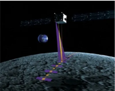
Figure 1.2 - Comparison between the swaths of the SMART-1 remote sensing instruments in lunar orbit: D-CIXS (32 · 12°), AMIE (5 · 5° or 2.5 · 1.25° colour frames) and SIR (400 point spectral continuous mapping). [2] ... 2

Figure 1.3 - Scheme of CCD field of AMIE/SMART-1 camera. ... 3

Figure 2.1 - First captured image of the moon's far side ... 7

Figure 2.2- Craters in northern Oceanus Procellarum on the Moon taken by Lunar Orbiter 5 ... 8

Figure 2.3 - Mosaic of the near side of the moon as taken by the Clementine star trackers. ... 10

Figure 2.4 - Epithermal counting rates poleward of ±70º ... 11

Figure 3.1 - AMIE map construction process ... 13

Figure 3.2 - Calibration process ... 14

Figure 3.3 - a) Zoomed area from image 9 of orbit 2141 before vertical stripes filtering and b) after filtering ... 16

Figure 3.4 - a) Flat field computed from in-flight data with grayscale adapted to filter areas. b) Adapted to unfiltered area. ... 17

Figure 3.5 – a) Full frame 10 from orbit 559 after dark current correction and before flat field correction. b) Full frame after flat field correction ... 17

Figure 3.6 – a) Correlation between frame observed and Hapke model brightness on AMIE map 6 and b) on AMIE map 61 ... 18

Figure 3.7 - Mosaic of AMIE map 10 using Hapke model brightness scaling ... 19

Figure 3.8 - Image 18 from orbit 40 with a corrupted block ... 20

Figure 3.9 - Full frame from image 1 of orbit 2865 with noticeable scattered light ... 21

Figure 3.10 - Scattered light compensation process ... 21

Figure 3.11 - RSC multilevel pyramidal structure example ... 22

Figure 3.12 - Example of an 8x8 pixel DCT matrix coefficients with the 1st and 4th bands highlighted [38] ... 24

Figure 3.13 - a) Block disposition over the full frame of the enhanced imaged. b) Block disposition on the vertical compensation image. c) Block disposition on the horizontal compensation image. ... 25

Figure 3.14 – Full frame 10 from orbit 559 without compensation and noticeable blocking effect ... 25

Figure 3.15 - a) Compensation weighting matrix for the vertical borders of blocking effect. b) Weighting matrix for the horizontal borders ... 26

Figure 3.16 – MPOS primary image weighting matrix ... 27

Figure 3.17 - Full frame 10 from orbit 559 after contrast balance ... 27

Figure 3.18 - Full frame 10 from orbit 559 after brightness balance ... 28

Figure 3.19 - Edge smoothing filter example ... 28

Figure 3.20 - a) Zoomed area of the full frame 10 from orbit 559 before smoothing filter. b) After smoothing filter. ... 29

Figure 3.21 - Coverage and resolution of AMIE full frame images [34] ... 30

Figure 3.22 - AMIE more equatorial maps coverage area ... 30

Figure 3.23 - a) AMIE North pole map area coverage and b) South pole map area coverage ... 31

Figure 3.24 - AMIE map data selection and ordering process ... 33

Figure 3.25 - Full frame 2 from orbit 771 with overexposed unfiltered area. ... 34

Figure 3.26 - AMIE dataset classification tool ... 35

Figure 3.27 - Illumination angles ... 36

Figure 3.28 – a) Map clusters order for maps north of 30°N and south of 50°S. b) Order for the more equatoria, maps. ... 37

Figure 3.29 - Coverage size ordering process ... 39

Figure 3.30 - Coverage computation example ... 40

Figure 3.31 - Image forward warping ... 40

Figure 3.32 - Map Builder in balance mode loaded with AMIE map 10 ... 42

Figure 3.33 - Map Builder in edition mode loaded with AMIE map 10 ... 43

Figure 3.34 – Map Builder balance process ... 44

Figure 3.35 - Full frame number 104 from orbit 81 isolated from map 10 ... 44

L

IST OF

T

ABLES

Table 2.1 - Detailed Information on Lunar Orbiters and Images collected [21] ... 9

Table 3.1 - AMIE maps detailed information ... 31

Table 3.2 - Classification of the Smart-1 AMIE full frame dataset... 34

L

IST OF

A

CRONYMS

AMIE - Advanced Moon Micro-Imager Experimenter ... 1

APS - Alpha Particle Spectrometer ... 11

CCD - Charge-Coupled Device ... 3

D-CIXS - Compact Imaging X-ray Spectrometer... 3

DCT - Discrete Cosine Transform ... 21

DGE - Doppler Gravity Experiment ... 11

DOG - Difference of Gaussians ... 22

EPDP - Electric Propulsion Diagnostic Package ... 3

ER - Electron Reflectometer ... 11

ESA - European Space Agency ... 1

FOV - Field of View ... 3

GRS - Gamma Ray Spectrometer ... 11

HIRES - High Resolution Camera ... 10

KaTE - Ka band TT&C (telemetry, tracking and control) Experiment ... 2

LIDAR - Laser Ranging System ... 10

LWIR - Long-Wave Infrared Camera ... 10

MAG - Magnetometer ... 11

MPOS - Modified Partially Overlapped Sub-block ... 21

MPOS-DCT ... See MPOS and DCT NASA - National Aeronautics and Space Administration ... 9

NIR - Near-Infrared Camera ... 10

NS - Neutron Spectrometer ... 11

RSC - Retinal-like Subsampling Contrast ... 22

RSIS - Radio Science Investigation with SMART-1 ... 3

SEPP - Solar Electric Primary Propulsion ... 2

SIR - SMART-1 Infrared Spectrometer ... 2

SMART-1 - Small Missions for Advanced Research in Technology-1 ... 1

SPEDE - Spacecraft Potential, Electron and Dust Experiment ... 3

SPICE - Spacecraft, Planet, Instrument, Camera-matrix, Event ... 31

US - United States ... 8

USGS - United States Geological Survey ... 10

USSR - Union of Soviet Socialist Republics ... 7

UVVIS - Ultraviolet/Visible Camera ... 10

XRF - X-ray fluorescence ... 3

1 I

NTRODUCTION

Mankind interest in space is present since the dawn of time. The blue of dark sky was always a giant origin of curiosity on Man’s soul that not even the evolution of knowledge and technology could erase. However, only on the 20th century there was finally a chance to explore it.

That chance came from war and the technological advances it brought. Until the 2nd World War rockets weren’t powerful enough to project any object into orbit. It only changed when the desire to overpower the enemy with bigger weapons at longer distances struck. Fortunately those advances found its way to different uses such as space exploration.

One of those missions propelled by pursuit of knowledge was the European Space Agency’s (ESA) Small Missions for Advanced Research in Technology-1 (SMART-1). The focus this thesis is the calibration, selection and mosaicing of the images captured by one of its instruments, the Advanced Moon Micro-Imager Experimenter (AMIE), with the intent to build a lunar atlas.

Below on this chapter the SMART-1 mission is described together with the detailed characteristics of the AMIE instrument, as well as the dataset issues and the thesis objectives. On chapter 2 a review of previous missions and relevance to the lunar mapping and atlas is presented. The methods applied to achieve the thesis objectives are detailed in the chapter 3 and finally on chapter 4 the discussion of results obtained and conclusion is presented.

1.1 SMART-1

M

ISSION

Launched on 27th September 2003 from the Guiana Space Centre in Kourou, French Guiana, SMART-1 was the first mission of the European Space Agency to the Moon. It was also the first and the last of the SMART mission series that was repurposed and renamed. The mission was planned to test new technologies for future missions and was part of the ESA strategy to build smaller low-cost spacecrafts [1].

It reached lunar capture on 15th November 2004 and science orbit of 400-3000Km on 15th March 2005. The mission nominal time was six months plus a one year extension in lunar science orbit [2]. The mission ended on the 3rd September 2006 on a controlled crash against the lunar surface in the Lacus Excellentiae region at a speed of 2 km/s and very shallow angle of incidence (~1°) [3].

The mission had both technical and scientific objectives, performing ten investigations based on three remote sensing instruments. Among the technical was performing a Laserlink experiment (the detection of a laser beam emitted by ESA/Tenerife ground station), flight demonstration of new technologies and on-board autonomy navigation. The science objectives were to image the lunar South Pole, permanent shadow areas (ice deposit), eternal light (crater rims), ancient lunar non-mare volcanism, local spectrophotometry as well as the physical state of the lunar surface and to map high altitude regions (the south) mainly at the far side (South Pole Aitken basin).

1.1.1 I

T

After being launched into orbit on board of an Ariane-5 rocket with other two satellites, it set a record by being the maiden mission to leave Earth orbit using only solar power, as well as setting the lowest fuel consumption per km for any Moon mission (but also the longest, 13 months) [4].

For that it used the Solar Electric Primary Propulsion (SEPP), an Hall Effect thruster that for its lightweight and small consumption is ideal for long-duration deep-space missions [5] [6]. As an addition, the SEPP by operating with a noble gas such as Xenon, that is known for good storability, also allows costs saving in safety procedures during ground operations.

The SMART-1 mission was also the first to use the Ka band for downlinking scientific data, latter used by other missions as the Mars Reconnaissance Orbiter and the Kepler space telescope. This system adopted the name Ka band TT&C (telemetry, tracking and control) Experiment (KaTE).

Figure 1.2 - Comparison between the swaths of the SMART-1 remote sensing instruments in lunar orbit: D-CIXS (32 · 12°), AMIE (5 · 5° or 2.5 · 1.25° colour frames) and SIR (400 point spectral continuous mapping). [2]

To accomplish its scientific goals the spacecraft was equipped with three remote sensing instruments for lunar study.

The Advanced Moon Micro-Imager Experimenter (AMIE) was an ultra-compact lightweight imaging system capable of capturing images in the visible and near infrared, which will be the basis of this thesis work and described in detail in chapter 1.1.1.1. The AMIE instrument was also used to perform the laserlink experiment that aimed at testing the feasibility of optical communications at long distances, as is the case of Earth to Moon. The interest of this experiment lies in the potential for greater data transfers during space missions.

the common element of Moon’s mantle and yet was poorly constrain in contemporary models. The study of the element distribution among the crust and surface would allow a perspective on the crustal differentiation and evolution [7]. As part of this study one of the main focuses was the South Pole Aitkin basin as it could have been dug through to expose materials from the Moon’s mantle.

The third equipment for lunar study was the Demonstration of a Compact Imaging X-ray Spectrometer (D-CIXS) which mapped the lunar surface for X-ray fluorescence (XRF) in the 0.5 to 10 keV range. This allowed for the bulk estimation of the elements Al, Mg and Si which has a direct bearing on the Giant Impact Theory of the Moon originating from the Earth. As well as the spectrometer the D-CIXS also included a Solar X-ray Monitor (XSM) which measured the Sun’s X-rays and to serve as a calibration for the D-CIXS data.

This study was the first XRF measurement since Apollo missions 15 and 16, and far more extensive as those only covered 9% of the Moon’s surface and were limited to the equatorial regions. More importantly was the first to give absolute elemental abundances instead of just elemental ratios.

Three other instruments were carried for navigation as well as for technological study, the Electric Propulsion Diagnostic Package (EPDP), Spacecraft Potential, Electron and Dust Experiment (SPEDE) and Radio Science Investigation with SMART-1 (RSIS). EPDP monitored the propulsion system, providing feedback for future solar electric engine designs. SPEDE was responsible for measuring the solar wind and besides the navigation purposes it was also used to perform studies while in lunar orbit. Finally the RSIS used AMIE’s high resolution and KATE to study the Moon’s libration with accurate orbit determination.

1.1.1.1 ADVANCED MOON MICRO-IMAGER EXPERIMENT (AMIE)

The Advanced Moon micro-Imager Experiment (AMIE) embedded on the SMART-1 spacecraft was an electronic miniaturised micro-camera and micro-processor built with the primary goal of imaging the lunar surface. The primary objectives were to imaging the South Pole permanent shadow areas, eternal light, ancient lunar non-mare volcanism, perform local spectrophotometry and physical state of the lunar surface and to map high latitudes regions (mainly at far side, e.g. the South Pole Aitken basin).

The imaging system was divided into two units, a camera unit and a dedicated electronics unit [8]. The camera was composed by a 5,3°x5,3° field of view (FOV) tele-objective and a 1024x1024 charge-coupled device (CCD) sensor. At the spacecraft apolune (at 3000km altitude from the Moon) the FOV produced an image resolution of 270m/pixel and at its perilune (at 300km of altitude over the South Pole) 27m/pixel image.

The sensor was divided into three spectral filtered areas of 750, 915 and 960nm, a smaller filtered area of 847nm also used for the Laserlink experiment and a 512x512 area without filtering, as is presented in Figure 1.3. While the 750 and 915nm filters were narrow band filters centred at the mentioned wavelengths and with a respective width of 10 and 30 nm, the 960nm filter was a high pass filter with steep transmission edge.

The electronic unit was responsible for the data control and power management of the camera. A Micro-DPU controlled the data processing and compression, image data storage into the data mass buffer, communication with the S/C and adaptation of the S/C supply voltage to the levels required by its electronics and the camera [8].

By capturing the same region with 3 different spectral bands the sensing unit allowed the discrimination of mafic materials (such as the pyroxenes and olivines that compose the mare on highland regions) by the Fe2+ absorption feature at 0.95μm. Also the imaging allowed the study of solar winds and micro-meteorites effect on the Moon’s surface as part of its maturation process.

On the 21st September 2010 the complete ESA’s SMART-1 data archives were released to the scientific community and among them were 31945 CCD full frames captured by AMIE instrument [4] [9] [10] [11] [12] [13] [14]. This dataset, the objective of this thesis, provides high-resolution mapping of the lunar surface, especially at the south polar area.

Since in the released AMIE dataset each captured image of the CCD is divided into several individual files, according to the filter it belongs, from now on the complete image will be referred to as a full frame. The individual filters images will simply be referred as frames or individual frames.

1.2 AMIE

D

ATASET

I

SSUES

Upon individually analysing the AMIE captured images several issues were discovered to have affected the dataset:

• The Van Allen radiation belts are at least two radiation zones of energetic charged particles around planet Earth at a distance between 650 and 650 000 km of altitude. [15] During Earth escape phase the SMART-1 spacecraft crossed the belts numerous times and was subjected to high doses of radiation which caused an increase in dark current accumulation on the CCD. This fact yielded the dark current compensation and camera flat field images, acquired during laboratory ground tests, inadequate to calibrate the mapping done during lunar an extended phase of the mission.

• When the instrument was switched on without capturing any image a considerable amount of dark current accumulated near the readout area, saturating that area of the captured frames.

• Many images suffer from a vertical stripes pattern with 8 pixel spacing and variable positioning. This effect is more noticeable on images with low light levels.

• A relatively large number of images presented corrupted blocks of pixels, where the pixels in that area present no discernable features while the remaining of the captured full frame has good quality.

• The filtered areas of the CCD full frame present a much lower contrast in comparison to the unfiltered portion. This is due to scattered light that got beneath the filters panel from the border with the unfiltered area.

1.3 O

BJECTIVES

With that goal in mind each issue mentioned in chapter 1.2 will be studied and processed to improve the calibration results and maximize images quality.

As the artificial satellite orbits around the Moon it also varies its position relatively to the Sun changing lighting conditions. Therefore, the images in the dataset present different illumination conditions that affect their quality. An adequate selection of the images to be projected into the maps will then have a severe effect on map’s quality and balance and should be addressed.

Earlier attempts to mosaic SMART-1 images showed that some full frame images present very different data values resulting in over brighten areas in the mosaiced map. Despite the images’ good quality the model brightness scaling could not compensate this effect and a solution should be found to allow the usage of these images.

2 S

TATE OF THE

A

RT

R

EVIEW

In this chapter a review of past space missions with Moon mapping objectives is made. Presented in chronological order, each of them represented not only a mark in history but also high scientific relevance at contemporary or current time. While some missions like Luna 3 have been surpassed by technologically more advanced missions, others as the Clementine mission are still being used as a reference in moon mapping.

The information presented in this review includes among others the technological equipment used and the mapping coverage, quality and resolution. These are key elements in the construction of an atlas. Below, on chapter 2.1 an individual review of each of the mapping missions with the mentioned relevant information is made.

2.1 I

NDIVIDUAL REVIEW

Here an extensive individual review of each of the most relevant lunar mapping missions or projects is presented in a chronological mission launch order.

2.1.1

Luna

3

The Luna 3 mission was a milestone in space exploration allowing mankind to see for the first time the moon’s far side. Using a complex imaging system to capture and relay images back to earth it provided a total of 29 images that might be considered low quality by today’s standards, but still a feat at the time.

The spacecraft, built by the Union of Soviet Socialist Republics (USSR), was launched on a Luna 8K72 rocket on October 4th of 1959 and three days later took the first picture, the one showed in Figure 2.1.

The imaging system consisted of a dual-lens camera, with a 500mm f/9.5 aperture and a 200mm f/5.6 aperture, as well as an automatic film processing unit, a scanner and a radio system. This system allowed the film to be converted into a frequency-modulated analog video format that could be relayed back to Earth. [16]

The 29 photographs captured covered 70% of the far side of the moon and were taken during a 40 minutes span. The first image was captured when the spacecraft was at a distance of 65567 km from the moon’s centre, and the last at 68785 km. During the process the telemetry was switched off to save power and no altitude information is available. [17]

The resulting pictures were very noisy and low resolution, but many features could still be recognized. It showed a very different terrain from the near side, very mountainous with only two dark regions.

In 1959 a book containing 28 out of the 29 Luna 3 images, 4 outline maps and lunar features description was assembled by the scientists of the main research centres in charge of analysing and processing the images retrieved by the mission. Named Atlas of the Far Side of the Moon [18] it gained popularity as it was the only published book containing images of the hidden side of Earth’s natural satellite for nearly 6 years.

2.1.2 L

O

The Lunar Orbiter project consisted of five identical unmanned spacecraft launched between 1966 and 1967. These were built with the primary goal of exploring for possible landing sites for the future United States’ (US) Apollo program. However, by the end of the third mission most of their objectives had been met and part of the remaining missions’ time was open for scientific exploration. [19]

Similar to other contemporary and previous mapping missions, these were equipped with a dual-lens camera, a film processing unit, readout scanner and a film handling apparatus. The type of equipment and setup was kept the same throughout the missions.

The lenses consisted of an 80mm, used for medium resolution, and a 610mm, used of high resolution shots. These were prepared so that shots taken from with the high resolution camera would coincide with the centre of the medium resolution frames. When shooting, the pictures of the different lenses were captured into adjacent areas of the same 70mm film supply, which was kept moving during exposure to compensate for the spacecraft’s velocity [20].

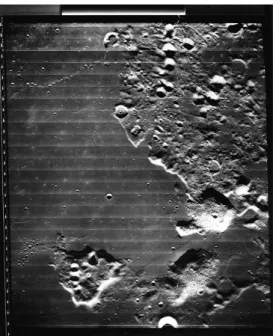
Figure 2.2- Craters in northern Oceanus Procellarum on the Moon taken by Lunar Orbiter 5

The Lunar Orbiter 1, 2 and 3 missions covered 22 possible landing sites near the equatorial area, taking pictures at low inclination and low altitude orbits for geological and topography study [19]. In addition they also took the opportunity to study the spacecraft’s trajectory, to improve the lunar gravity definition, and measurements of micrometeorites and lunar radiation flux for performance improvement.

The final Lunar Orbiter mission was meant to complement the previous missions, taking additional high quality images of possible landing sites for the future missions and scientifically interesting sites at highly inclined orbits (85 degrees, as used in mission 4). It focused primarily on 68 photo sites during its orbits, 45 on the near side and 23 on the far side, with a resolution between 20 meters (for medium resolution frames) and 2 meters (for high resolution). In Figure 2.2, despite visible lines created during readout, is noticeable the good quality of the images captured by the last spacecraft of the Lunar Orbiter missions.

By the end of the last Lunar Orbiter mission 99% of the entire moon’s surface had been mapped with a resolution of 60 meters or better. The summary of captured images and flight information of the entire Lunar Orbiter Project is presented in Table 2.1.

Table 2.1 - Detailed Information on Lunar Orbiters and Images collected [21]

Photographic Parameters Lunar Orbiter 1 Lunar Orbiter 2 Lunar Orbiter 3 Lunar Orbiter 4 Lunar Orbiter 5

Launch Date 10 Aug 1966 10 Nov 1966 05 Feb 1967 04 May 1967 01 Aug 1967 Periselene (km) 40.5 41 44 2668 97 Aposelene (km) 1857 1871 1847 6151 6092 Inclination (deg) 12 12 21 85.5 85 Period (h) 3.5 3.5 3.5 12 8.5,3.0 Impact date 29 Oct 1966 11 Oct 1967 10 Oct 1967 31 Oct 1967 31-Jan-68 Impact coordinates 7 N, 161 E 3 N, 119.1 E 14.32 N,

92.7 W ??, 22-30 W

2.79 S, 83 W Acquisition dates 18-29 Aug ₁₉₆₆ 18-25 Nov ₁₉₆₆ 15-23 Feb ₁₉₆₇ 11-26 May ₁₉₆₇ 06-18 Aug ₁₉₆₇

Quantity of frames

High

resolution 42 609 477 419 633 Medium

resolution 187 208 149 127 211

Altitude range for photography (km) 44 - 1581 41 - 1519 44 - 1463 2668 - 6151 97 - 5758

Highest resolution

Periselene

(m) 8 1 1 58 2 Aposelene

(m) 275 33 32 134 125

Framelet width at periselene (m)

High

resolution 200 170 185 11350 420 Medium

resolution 1500 1300 1400 85100 3200

In 1971 David Bowker and Kenrick Hughes of the National Aeronautics and Space Administration’s (NASA) Langley Research Center published the Lunar Orbiter photographic atlas of the Moon [22]. In this book they assembled 675 plates of the Lunar Orbiter missions into a detailed atlas with annotations on the named moon’s features. It included plates both from the near and the far side and was mostly based on the fourth mission survey.

The Lunar Orbiter photographic atlas of the Moon became a reference for lunar topography for its high quality pictures and detailed information. Today due to its rarity a used copy is highly valued, being nowadays found for sale at prices above 400 US dollars.

2.1.3 C

a variety of sensing techniques, consistently expressed in the previous 20 years [23]. Therefore, its science objectives were defined as to obtain topographic imaging, altimetry data and multispectral imaging of the lunar surface. The Clementine mission was the first to acquire a digital image data set of the moon.

The spacecraft was equipped with four cameras: an ultraviolet/visible camera (UVVIS), a long-wave infrared camera (LWIR), a high resolution camera (HIRES) equipped with a laser ranging system (LIDAR) and a near-infrared camera (NIR) [24]. As an addition it also had two star-tracker cameras used essentially for altitude determination, but that could also be used as wide-field cameras for scientific or other operational purposes.

The UVVIS camera was a CCD imager with a six filter wheel, with filters centred from 415 up to 1000nm and a broad-band filter covering from 400 to 950nm. The NIR also had a six filter wheel but with filters ranging from 1100 up to 2780nm. The LWIR had a bandwidth from 8000 to 9500nm and the HIRES camera a broadband filter from 400 to 800nm, as well as four other filters centred from 415nm up to 750nm. In addition to the mapping cameras it also carried a charged-particle telescope, which had the objective of studying the solar and magnetospheric energetic-particle environment.

Arriving at Earth’s natural satellite on 19 of February of 1994 it remained operational during 71 days with a 5-hour elliptical polar orbit. During this period took 620 000 high resolution and 320 000 mid-infrared thermal images to an approximated total of 2.8 million images, as well as mapped the lunar topography with its laser-ranging system. It covered 38 million square kilometres mapping the moon in 11 visible and infrared colours with an average resolution of about 200 meters per pixel.

Figure 2.3 - Mosaic of the near side of the moon as taken by the Clementine star trackers.

Besides the mapping objectives, it also provided with more accurate spacecraft position tracking data, used to improve the lunar gravitational field model. Despite the already provided data from the Apollo and Lunar Orbiter earlier missions these were either only restricted to equatorial regions or the tracking resolution at the time was only enough to provide a fairly coarse potential field model. [25]

Among the relevant scientific discoveries was the relevance of the South Pole-Aitken basin. Being the largest basin on the Moon, with more than 2500 km in diameter and 13 km of depth, it was found that has maintained much of its original relief [25]. Not only was in an amazing preservation state but the compositional data showed that its floor has the largest composition anomaly on the far side, having significantly higher quantities of iron and titanium contents than any other location.

2.1.4 L

P

The Lunar Prospector spacecraft was a complementary low-budget mission of the previous Clementine. While the later was equipped mostly with imaging cameras the Lunar Prospector equipment was essentially composed by spectrometers to study the Moon’s composition, as well as equipment to analyse the gravity and magnetic field [27]. Launched on 7 January 1998 by an Athena 2 rocket it reached Moon’s orbit 105 hours later, maintaining operations for 570 days.

Aboard the spacecraft were a Gamma Ray Spectrometer (GRS), a Neutron Spectrometer (NS), a Magnetometer (MAG), an Electron Reflectometer (ER), an Alpha Particle Spectrometer (APS), and a Doppler Gravity Experiment (DGE) [28].

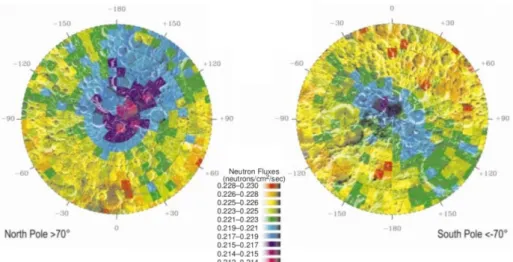
Figure 2.4 - Epithermal counting rates poleward of ±70º

Among the most relevant scientific studies was the existence of water on the Moon’s polar regions, subject which had once more been raised upon the data collected from Clementine mission. Maps of epithermal and fast-neutron fluxes measured by the Lunar Prospector were used to search for deposits of hydrogen in both poles. [29]

The data was consistent with water ice deposits buried beneath 40 cm of dry regolith in an estimated area of 1850 km² at both poles, as shown by epithermal counting rates in Figure 2.4. In an attempt to further confirm this, a crater near the South Pole was chosen as the controlled crash site for the end of the mission while was being observed by Earth-based observatories and the Hubble Space Telescope. [30] Although a successful crash was achieved the data collected showed observable water signature.

2.2 S

YNTHESIS

As mentioned before, the URSS Luna 3 space mission was the first to photograph the Moon’s far side. Launched in 1959 at the beginning of the space race, the technology it carried was only capable of producing a small number of blurry low resolution images, covering 70% of the Moon’s far side. This did not stop them from being assembled and used as part of the Atlas of the Far Side of the Moon [18].

photographic atlas of the Moon [22] with detailed annotations by assembling 671 plates of the Lunar Orbiter dataset.

The next extensive lunar mapping occurred only 27 years later in 1994. The Clementine mission included several cameras in the ultraviolet, visible and infrared spectrum of light, high resolution camera, laser raging system along with equipment for other scientific studies. It captured approximately 2.8 million images and the mapping achieved is currently still used as a reference for other space missions (the SMART-1 included). The captured visible/ultraviolet images are broadly used on Moon atlas inclusively the most currently widely spread digital lunar atlas, the Google Moon.

3 M

ETHODOLOGY

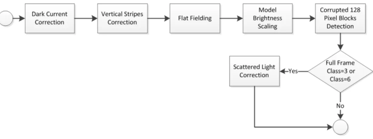
In this chapter the methods applied with the goal of achieving the best possible mosaiced lunar maps, as well as the objectives defined in chapter 1.3, are described in detail. The information is presented in the order in which the process should be executed, following the flowchart in Figure 3.1. Its practical implementation was achieved using the mathematical computational environment MATLAB® [31].

Figure 3.1 - AMIE map construction process

It begins by improving the AMIE dataset full frames by calibrating each one (chapter 3.1). This step removes the effect of dark current, electronic noise, pixel-by-pixel sensitivity differences and scattered light that penetrated between the filters and CCD. During the calibration each full frame is also checked for corrupted blocks of pixels and each full frame’s brightness is scaled for map illumination balance.

In chapter 3.2 the map organization of the AMIE Moon Atlas is detailed. Besides the map division is also described the map area coverage, the type of projection used and the dataset coverage on each of the maps. It is also discussed the information required for the full frames geometric computation and its pointing accuracy.

The map mosaicing in chapter 3.3 includes the projection methods applied, the full frames classification according to their visual quality and their organization order for projection. Finally the Map Builder is the tool responsible for handling the execution process of the methods described in the previous chapters, editing the mosaiced maps and performing the final needed brightness and contrast adjustments (chapter 3.4).

3.1 C

ALIBRATION

The calibration process of the AMIE CCD full frames aims at achieving brightness and contrast balanced images while reducing the noise. To do so the standard calibration of the camera must be done. That includes the removal of the dark current effects (chapter 3.1.1) as well as the removal of sensitivity differences between pixels, in the process referred to as Flat Fielding (chapter 3.1.3).

As an addition several other processes had to be introduced to address the dataset issues detected in chapter1.2. The Vertical Stripes Correction of chapter 3.1.2 applies a weighted line median filter as a method to remove the stripes pattern present in some full frames at low light, without compromising image quality. Chapter 3.1.5 applies a detection method to mark and exclude the 128 by 128 corrupted blocks of pixels from further processing and mosaicing while maintaining the rest of the uncorrupted full frame. The lower contrast in the filtered areas of the full frame caused by the scattered light is addressed in chapter 3.1.6 in a more direct to the problem approach that includes contrast enhancement.

Figure 3.2 - Calibration process

The complete calibration process is described in Figure 3.2 with the different blocks presented according to its execution order. The Scattered Light Correction is only applied in the cases where the full frame has been classified with class 3 or class 6, those classes that mark both filtered and unfiltered areas of the full frame as usable. The AMIE full frame classification is described in chapter 3.3.1.1.

3.1.1 D

C

Dark current builds up in CCD sensors whether they are exposed to radiance or not, producing noise with random pixel accumulation that affects the quality of the acquired frames. This is caused by thermally created electrons and holes that build up in the pixels, having a direct relation with CCD temperature and exposure time. To remove this pattern a dark image is used (or a combination of dark images) and bias image, which is an image with no exposure time to compensate for the noise created by the CCD electronics. Therefore, the 𝐷 data number for an acquired pixel will be defined by equation (3.1)

𝐷=𝑑₀+𝐵 ∙ 𝑓(𝑇) +𝑆 ∙ 𝑓(𝑇)∙ 𝑡_𝑒+𝐶 ∙ 𝐼 ∙ 𝑡_𝑒 (3.1)

Where 𝑑₀ is a fixed data number offset (8 in the SMART-1 AMIE case), 𝐵 the bias built up during readout, 𝑓(𝑇) the function describing the temperature dependence, 𝑆 the dark current during exposure, 𝑡_𝑒 the exposure time, 𝐶 the radiance conversion factor and 𝐼 the incoming radiance. The temperature function and exposure time are pixel independent, the remaining are not.

In order to assess the dark current contribution a frame with incoming radiance 𝐼= 0 is needed, which results in the simplified equation (3.2). The frame is then subtracted to the original 𝐷 data numbers to obtain the corrected frame (equation (3.3)).

𝐷𝐷𝑎𝑟𝑘=𝑑0+ (𝐵+𝑆 ∙ 𝑡𝑒)∙ 𝑓(𝑇) (3.2)

𝐷𝐶𝑜𝑟𝑟=𝐷 − 𝐷𝐷𝑎𝑟𝑘 (3.3)

During Earth’s escape phase the CCD sensor suffered an increased accumulation of dark current due to numerous radiation belt crossings, leaving the previously laboratory acquired dark frames inadequate to perform the correction. A new set of dark frames were acquired from in-flight data of dark sky observations during the lunar and extended phase of the mission. [32] To reduce the effect of noise and possible pixel errors a total of 154 dark sky images were used. To remove the temperature contribution an estimation was made using equations (3.4) and (3.5).

𝑓(𝑡) =�𝑇

𝑇0� 3 2

∙ 𝑒𝑥𝑝 �𝐸𝑔(𝑇0)

2.𝑘.𝑇₀−

𝐸𝑔(𝑇)

𝐸𝑔(𝑇) = 1.11557−

7.021 . 10−4.𝑇2

1108𝐾+𝑇 (3.5)

Where 𝑇₀ is a reference temperature (which was chosen to be

𝑇0= 273.15𝐾) and 𝑘 the Boltzmann constant (𝑘= 8.6171∙10−5𝑒𝑉/𝐾).

After removing the offset 𝑑₀ and temperature𝑓(𝑡) the dark frames have only the contribution of the bias 𝐵, which is independent of exposure time, and the dark current slope 𝑆 (equation (3.6)). A frame with null exposure time is not achievable, but the same result can be obtained by interpolating two or more full frames (on this case the 154 chosen dark sky images) to an exposure time 𝑡_𝑒= 0 on each pixel. By doing this a bias plus offset (𝑑₀+𝐵) estimation can be retrieved, as well as the slope 𝑆. Having all the elements needed to obtain the dark frame 𝐷_{𝐷𝑎𝑟𝑘}, the correction is then simply done using equation (3.3) as previously mentioned.

𝐵(𝑥,𝑦) +𝑆(𝑥,𝑦)∙ 𝑡_𝑒=D(𝑥,𝑦,𝑘)− 𝑑0

𝑓(𝑇) (3.6)

When the instrument was switched on without capturing any image a considerable amount of dark current accumulated near the readout area, saturating that area of the frames. This charge was swept away whenever a new frame was captured. When this problem was detected a procedure of capturing a frame without downloading it was implemented by ESA’s operators, but still some of the dark frames used to estimate the dark correction suffer from this problem, propagating it to the corrected images. This effect is clearly visible at the top of Figure 3.5.

To avoid extending the effect to the AMIE map mosaics, the top 128 pixels of each full frame are removed before the scattered light compensation and are not included in the further processing or mosaicing.

3.1.2 V

S

As can be seen on Figure 3.3, many images suffer from a vertical stripes pattern with an 8 pixel spacing and variable location on the CCD, especially at low light levels. This variation on the location makes its removal not so trivial. A relation between the pattern and the interference from the triggering of serial CCD read out has been suggested but no confirmed explanation has been found [32]. The same type of equipment with newer firmware version does not seem to suffer from this effect.

A seven pixel horizontal line median filter was first implemented as a solution for the pattern at the cost of some image definition. To reduce this definition loss the filtered and unfiltered image were then weighted through equation (3.7), where 𝐷_𝑓 and 𝐷 are the filtered and unfiltered images, and 𝑐 the weighting factor from equation (3.8).

𝐼=𝑐.𝐷_𝑓+ (1− 𝑐).𝐷 (3.7)

𝑐=𝑒−�

𝐷𝑓

64�

2

a)

b)

Figure 3.3 - a) Zoomed area from image 9 of orbit 2141 before vertical stripes filtering and b) after filtering

Compared with the simple filtering, this method allows the removal of the vertical stripes while preserving the brighter parts without degradation.

3.1.3 F

F

After dark current correction the 𝐷_{𝐶𝑜𝑟𝑟} frame is simply defined by equation (3.9). Having a laboratory blank image with a known radiance 𝐼₀, constant throughout the pixels, and the exposure time allows recovery of the incoming radiance of the corrected frame. This is achieved by dividing by the laboratory blank image, as presented in equation (3.10). This laboratory blank image is usually referred to as flat field.

𝐷𝐶𝑜𝑟𝑟=𝐶 ∙ 𝐼 ∙ 𝑡𝑒 (3.9)

𝐼=𝐷𝐶𝑜𝑟𝑟

𝐷𝑓𝑙𝑎𝑡.

𝑡𝑒0

𝑡𝑒 .𝐼0 (3.10)

The mentioned increase in dark current accumulation from Earth’s radiation belt rendered the flat fields previously acquired in laboratory also unable to provide with an adequate correction. Therefore an in-flight flat field was required.

a) b)

Figure 3.4 - a) Flat field computed from in-flight data with grayscale adapted to filter areas. b) Adapted to unfiltered area.

As it can be seen on Figure 3.4 a) the computed flat field from in-flight data has areas with very different brightness levels. That is so it can compensate for intensity attenuation of each of the filters and achieve an usable, visually balanced CCD full frame. It is also noticeable the extreme attenuation the filters caused in comparison with the unfiltered area of the full frame. The brightness difference is so large that no greyscale has enough dynamic to show both areas of the flat field simultaneously, and have to be separately scaled for preview.

a) b)

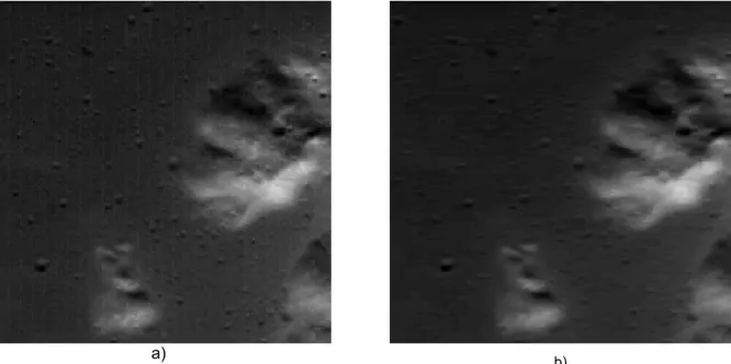
Figure 3.5 – a) Full frame 10 from orbit 559 after dark current correction and before flat field correction. b) Full frame after flat field correction

In the same figure it is also noticeable the contrast difference between filtered and unfiltered areas due to the scattered light. Its large variability across the dataset full frames makes it impossible for the flat field to compensate for this effect.

3.1.4 M

B

S

To compensate the different illumination conditions of the images throughout the maps, each frame is scaled using the Hapke reflectance model [33]. The formula for the reflected radiance is given by equation (3.11), where 𝜔 is the soil albedo, 𝜇₀ the cosine function of the incidence angle, 𝜇 the cosine function of the emission angle, 𝑔 the phase angle and 𝑑 the distance to the sun. The function B is expressed by equation (3.12) and represents the opposition peak, with 𝐵₀ and ℎ being two parameters for the height and angular width.

𝐼= |𝜇0| (|𝜇₀| +𝜇).�

1𝐴𝑈

𝑑 �

2

. [𝑝(𝑔). (1 +𝐵(𝑔)) +𝐻(|𝜇₀|).𝐻(𝜇)−1] (3.11)

𝐵(𝑔) = 𝐵0

�1 +tan_{ℎ �}�𝑔2� (3.12)

The Chandraeskhar H-function in equation (3.13) was used to approximate the multiple scattering radiance and equation (3.14), suggested by Michael Küppers, the single scattering.

𝐻(𝑥) = 1 + 2𝑥

1 + 2𝑥√1− 𝜔 (3.13)

𝑝(𝑔) =𝜋

2

5 .�

sin𝑔+ (𝜋 − 𝑔). cos𝑔

𝜋 +

(1−cos𝑔)2

10 � (3.14)

To equalize the frames each image is divided by its modelled radiance 𝐼, with the variable factors chosen to be 𝐵₀= 0 and 𝜔= 0.12.

a) b)

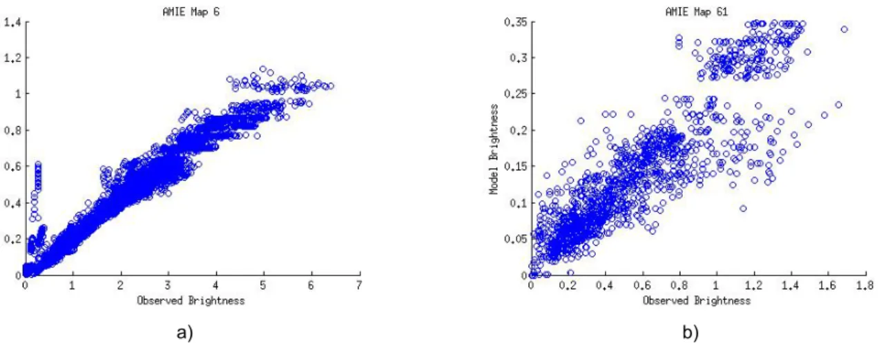
Figure 3.6 – a) Correlation between frame observed and Hapke model brightness on AMIE map 6 and b) on AMIE map 61

angles as noticeable on Figure 3.6 where the observed and the modelled brightness of the frames are compared.

On map 6 (Figure 3.6 a)) which has a medium incidence angle (around 45 degrees) the correlation value between the two is 0.9859 and obtains a good brightness balance on the mosaicked map. On the other hand map 61 (Figure 3.6 b)) has a higher incidence angle (around 75 degrees) and its correlation value is inferior to the previous one having a value of 0.9452. Also its mosaicked map does not have a visually balanced brightness. Trying to further tune the Hapke model parameters did not seem to improve the correlation results.

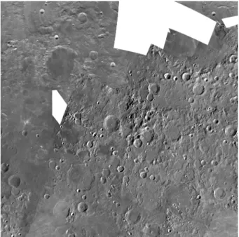
Figure 3.7 - Mosaic of AMIE map 10 using Hapke model brightness scaling

Some full frame images also show an abnormal data median value compared to the rest of the AMIE dataset. Despite having good quality images, these full frames cannot obviously be balanced with the rest of the mosaiced maps by the brightness model scaling, as seen on map 10 presented on Figure 3.7.

For the cases where the limitations of this chapter’s brightness scaling severely affects the mosaiced map an empirical scaling method has been implemented and is described in chapter 3.4.3.

3.1.5 C

128

P

B

Figure 3.8 - Image 18 from orbit 40 with a corrupted block

Since most of these blocks had no visible features and extremely larger data numbers compared to the rest of the frame it severely affected any operation on the frame that included them (e.g. mean, median, maximum value…), albeit their constant positioning allows for a possible detection and removal from mosaicing.

To use the frame without being affected each block is tested for corruption using the steps:

• The frame is divided into an 8 by 8 grid, leaving 64 individual blocks of 128 pixels.

• The mean, minimum and maximum is computed for each block.

• The mean of the full frame is computed, excluding areas of the where the corresponding block has a mean value inferior to 0.

• Each block is then marked as corrupted if its mean value is the same as the maximum or the minimum, its maximum value is less than or equal to 0 and if its mean value is largely greater than the mean value of the entire full frame.

For the comparison between the block and the full frame mean it was chosen to mark as corrupted blocks where its mean was 15 times bigger than the frame value. This value allows to correctly detect most of the blocks without false positives from frames with low angle illumination, which are mostly composed of large dark areas and small visible mountainous tops. The result of the test is then subsequently used to exclude the marked areas from any required computation.

Despite the exclusion of the detected corrupted areas there are still a smaller number of corrupted blocks that have no discernible variation of data numbers in relation to the rest of the frame. For those a detection method could not be obtained.

Using the dataset classification process described on chapter 3.3.1.1 the full frames with detectable corrupted blocks were marked as damaged. After the process was complete 530 full frames were detected and marked as damaged.

3.1.6 S

L

If the scattered light had a constant effect on all frames it would have been removed by the flat fielding process, but that is not the case. The noticeable brighter filters from Figure 3.9 are an indication of above average scatter and, as there is above cases, there are also frames with below average and darker filters area making its removal difficult.

Figure 3.9 - Full frame from image 1 of orbit 2865 with noticeable scattered light

A process for the scattered light removal has previously been proposed by Björn Grieger [34]. This method had the tendency to overestimate the amount of scattered light, yielding too dark filters areas. Therefore, a different approach has been taken to this problem.

Figure 3.10 - Scattered light compensation process

Since the main problem caused by the scattered light is the reduced contrast on the filtered areas, in comparison to the unfiltered areas, a more direct approach can be taken by increasing the contrast where needed. As Figure 3.10 describes, to do so first the contrast of both areas is measured and compared. If needed, the filters area of the frame is then increased in contrast until both areas have similar values. When this is achieved the possible differences in brightness and edge between the filtered and unfiltered areas are adjusted.

The process is described in detail below. Chapter 3.1.6.1 details the Retinal-like Subsampling Contrast (RSC) which is the contrast measurement algorithm used to compare the contrast between the areas of the full frame.

Finally, in chapter 3.1.6.3 the brightness adjustments needed to compensate for the contrast enhancement are detailed.

3.1.6.1 RSCCONTRAST MEASURE

In order to compare the contrast of different images a contrast measure which provides a result that highly correlates with the human optical perception of contrast is needed. However, the measurement and evaluation of contrast and contrast changes in arbitrary images are not uniquely defined in the literature [35], and perceptual contrast is strongly defined by the contextual influence on the observer task and experience.

A few different methods were tested for this purpose but the one found to be the better fit was defined as Retinal-like Subsampling Contrast (RSC) [36]. The version used and described below is a slightly modified one with a one value per image measurement result.

To achieve the contrast evaluation the image is transformed into a multilevel pyramidal structure. Each level is obtained by subsampling the image from the previous level to half the size, starting from the original image. In this case each image was subsampled into levels, until one of its dimensions fall beneath 4 pixels.

Figure 3.11 - RSC multilevel pyramidal structure example

𝐷𝑂𝐺(𝑥,𝑦) =𝑅_𝑐(𝑥,𝑦)− 𝑅_𝑠(𝑥,𝑦) (3.15)

Then, for each level, the computation of the difference of Gaussians (DOG) is performed. The conventional DOG model, presented in equation (3.15), is defined by the difference between the central 𝑅_𝑐 and the surround 𝑅_𝑠components. The components 𝑅_𝑐 and 𝑅_𝑠 are the level image after being filtered with two different Gaussian filters, with radius 𝑟_𝑐 and 𝑟_𝑠.respectively. This is because it assumes a retinal ganglion cell or an LGN neuron response is only dependant on the luminance difference. After the light adaptation process a neuron is also dependant on the local luminance average. Therefore, the model should be adapted. Tadmor and Tolhurst [37] suggested equation (3.16) as solution.

𝐷𝑂𝐺𝐿𝑇𝑇(𝑥,𝑦) =𝑅𝑐

(𝑥,𝑦)− 𝑅_𝑠(𝑥,𝑦)

𝑅𝑐(𝑥,𝑦) +𝑅𝑠(𝑥,𝑦)

(3.16)

The contrast of each level image will then be the average value along the modified 𝐷𝑂𝐺_𝐿𝑇𝑇 (equation (3.17)) on the positions where the level image has data values above a defined minimum value.

𝐶𝐿=

1

𝑛𝑠𝑢𝑚× � � 𝐷𝑂𝐺𝐿

𝑇𝑇_(𝑖,𝑗)

𝑗𝑚𝑎𝑥

𝑗=1

𝑖𝑚𝑎𝑥

𝑖=1

[𝐼𝑚𝑔_𝐿(𝑖,𝑗) >𝑚𝑖𝑛𝑉𝑎𝑙] (3.17)

𝐶𝑅𝑆𝐶₌1

𝑛×� 𝐶𝐿

𝑛

𝐿=1

(3.18)

The overall contrast of the original image 𝐶𝑅𝑆𝐶 will be the average of the previously acquired levels contrast values, as expressed by (3.18) with 𝑛 being the number of levels. As radius for the Gaussian filters were used 𝑟_𝑐 = 2 and 𝑟_𝑠= 4.

3.1.6.2 MPOS-DCTCONTRAST ENHANCEMENT

Image enhancement techniques can be divided into direct and indirect enhancement methods. Indirect refer to methods that enhances the image contrast without measuring its contrast, while direct methods establish a contrast measure criterion and improve the image contrast directly according it. [38]

It can also be made the distinction between global and local contrast enhancement. Global methods are usually less complex and computational faster, but achieve less satisfying results as they treat the whole image as a block and make no distinction between different areas. Local enhancement methods divide the image into different areas with far more satisfying results, but their complexity can be a problem when real-time computation is needed or speed is a factor.

Since the dataset include a large number of full frames the processing time is an aspect that must be taken into account, otherwise the time needed to mosaic an AMIE map will be too long. The adopted technique is a direct local enhancement technique that is a combination of modified versions of methods proposed by Tang [38] and Kim [39]. It uses the discrete cosine transform (DCT) as a basis for contrast enhancement and a modified partially overlapped sub-block (MPOS) for local enhancement block effect removal. The DCT enhancement method offers the same enhancement quality but with less computation requirements than other equivalent methods.

Below the discrete cosine transform enhancement is described in detail (chapter 3.1.6.2.1) as well as the modified partially overlapped sub-block (chapter 3.1.6.2.2).

3.1.6.2.1 DCTCONTRAST ENHANCEMENT

The method proposed by Tang [38] takes advantage of DCT-based image compression standards such as JPEG, MPEG2 and H.261, in which the images are divided into 8x8 non-overlapping pixel blocks and computed the two dimensional DCT of each block. By modifying the DCT coefficients the image contrast can be improved without affecting the compression and even reducing storage requirements. Despite being thought to use the compression standards the method is not limited in its use, and can be widely applied to any image. In this case, the contrast enhancement is applied without the limitation of 8 by 8 pixel blocks made by the compression standards.

Figure 3.12 - Example of an 8x8 pixel DCT matrix coefficients with the 1st and 4th bands highlighted [38]

This provides a natural way of measuring contrast by using Peli’s [35] contrast definition, that states that human contrast perception is based on the difference between the high and low frequency content. By grouping the coefficients into frequency bands the contrast can then be defined using equation (3.19), where 𝐸_𝑛 is the average amplitude over the band n, and defined by equation (3.20).

𝐶𝑛=_∑𝐸𝑛_𝐸 𝑡 𝑛−1 𝑡=0

(3.19)

𝐸𝑡=∑

|𝑑_𝑘+𝑙|

𝑘+𝑙=𝑡

𝑁 (3.20)

Since the objective is to increase the contrast uniformly over all frequencies, the new contrast coefficients 𝐶���_𝑛 will be related to the previously acquired coefficients 𝐶_𝑛 by the constant contrast increase value 𝜆. Solving equation (3.21) allows finding that the new DCT 𝑑�����_𝑘,𝑙 matrix coefficients are given by equation (3.22).

𝐶𝑛

���=𝜆.𝐶_𝑛 (3.21)

𝑑𝑘,𝑙

�����=𝜆.𝐻_𝑘+𝑙.𝑑_𝑘,𝑙, 𝑛 ≥1 (3.22)

Where,

𝐻𝑘+𝑙=∑ 𝐸𝑡

�

𝑛−1 𝑡=0

∑𝑛−1𝑡=0𝐸𝑡

, 𝑘+𝑙 ≥1 (3.23)

After the 𝑑�����_𝑘,𝑙 matrix coefficients are computed the inverse discrete cosine transform is performed and the contrast improved image recovered.

The DCT contrast method allows for both contrast intensification and reduction. For 𝜆 values above 1 the contrast is intensified. For values between 0 and 1 the image contrast is reduced.

3.1.6.2.2 MPOSLOCAL CONTRAST ALGORITHM

Local contrast enhancement techniques have the tendency to suffer from blocking effects, where borders between adjacent blocks have different brightness levels. As it can been seen on Figure 3.14, this has a tendency to become more noticeable as the block pixel size increases. To compensate for this effect a modified method based on Kim’s [39] previously proposed one was implemented. It uses an image weighting system between images with three different blocks dispositions, instead of the simple overlapping blocks proposed. This allows for bigger block sizes without the blocking affect becoming significantly noticeable, which reduces the needed computation.

a) b) c)

Figure 3.13 - a) Block disposition over the full frame of the enhanced imaged. b) Block disposition on the vertical compensation image. c) Block disposition on the horizontal compensation image.

To begin the process the image is divided into 128x128 non-overlapping pixel blocks and on each block the DCT contrast enhancement is applied. Taking into account that the top 128 pixels of the images have been removed due to dark current accumulation this creates 7 by 8 matrix of blocks over the image.

To compensate for the vertical borders of the blocking effect another pass is made over the image now with half of the block size (in this case 64 pixels) of horizontal phase difference from the first. To compensate for the horizontal borders the same process is made but with half of the block size of vertical phase difference instead.

Figure 3.14 – Full frame 10 from orbit 559 without compensation and noticeable blocking effect

The effect of the brightness difference between filtered and unfiltered areas needs to be removed from the process to avoid undesirable propagation. To ensure this, the problematic areas of the compensation are weighted out. These areas are the large strips with 0 value on the weighting matrixes of Figure 3.15.

a) b)

Figure 3.15 - a) Compensation weighting matrix for the vertical borders of blocking effect. b) Weighting matrix for the horizontal borders

𝐼=𝐼₀.𝑊_𝑖𝑚𝑔+𝑊_{𝐶𝑜𝑚𝑝}. (𝐼_𝑉.𝑊_𝑉′+𝐼_𝐻.𝑊_𝐻′) (3.24)

The three images are weighted using equation (3.24), where 𝐼₀ is the uncompensated contrast enhanced image, 𝐼_𝑉 and 𝐼_𝐻 the blocking effect compensation images for vertical and horizontal borders and 𝑊_𝑖𝑚𝑔and 𝑊_{𝐶𝑜𝑚𝑝} the weighting matrixes for contrast improved image and the overall blocking effect compensation.

𝑊𝑉′ and 𝑊𝐻′ are the balanced weighting matrixes, as they need to be balanced against each other to mathematically ensure that the compensation is not weighted above 1. This is simply achieved by equations (3.25) and (3.26), with 𝑊_𝑉 and 𝑊_𝐻 being the unbalanced matrixes of Figure 3.15.

𝑊𝑉′(𝑥,𝑦) = 𝑊𝑉

(𝑥,𝑦)

𝑊𝑉(𝑥,𝑦) +𝑊𝐻(𝑥,𝑦)

(3.25)

𝑊𝐻′(𝑥,𝑦) = 𝑊𝐻

(𝑥,𝑦)

𝑊𝑉(𝑥,𝑦) +𝑊𝐻(𝑥,𝑦)

(3.26)

The compensation weighting matrix is then the maximum value between the vertical and horizontal weighting matrixes on each position (equation (3.27)). The contrast enhanced image weighting matrix is then the inverse value on each of the positions of the compensation matrix (equation (3.28)).

𝑊𝐶𝑜𝑚𝑝(𝑥,𝑦) = max �𝑊𝑉(𝑥,𝑦); 𝑊𝐻(𝑥,𝑦)� (3.27)

𝑊𝑖𝑚𝑔(𝑥,𝑦) = 1− 𝑊𝐶𝑜𝑚𝑝(𝑥,𝑦) (3.28)

weighting matrix is reconstructed through the inverse process. In Figure 3.16 the final weighting matrix 𝑊𝑖𝑚𝑔 can be seen.

Figure 3.16 – MPOS primary image weighting matrix

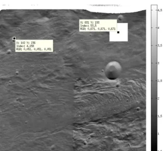
After all the weighting matrixes are produced, the final contrast improved image can be recovered using equation (3.24). The contrast balanced full frame is then the combination of the enhanced filtered area of the full frame and original unfiltered area. As noticeable in Figure 3.17, albeit in some images there is still a small effect from scattered light near the border between filtered and unfiltered areas, its effect has been greatly reduced and full frame appears visually more balanced.

Figure 3.17 - Full frame 10 from orbit 559 after contrast balance

3.1.6.3 BRIGHTNESS ADJUSTMENTS

After the full frame has been contrast measured by the RSC contrast measure and the contrast difference of filtered and unfiltered reduced by MPOS-DCT contrast enhancement a mean brightness difference is present between both areas. This is created by the scattered light effect previously existent on the frame as well as the process of contrast enhancement.

Figure 3.18 - Full frame 10 from orbit 559 after brightness balance

Before it is complete there is yet a visually unpleasant line edge between filtered and unfiltered derived from the previously described brightness adjustment. A smoothing filtered passed only over the edge is applied to make it less noticeable.

150 155 158 2 5 165 172 165

165 170 168 166 164 162 160 162 145 131 135 139 143 147 151 154

140 142 153 10 7 133 176 168

Figure 3.19 - Edge smoothing filter example

Figure 3.20 a) shows the prominent low brightness edge only covers the two pixels closest to the frontier between areas on each side. The mean value between the third pixel on each side (underlined on Figure 3.19) of the frontier is computed and divided by the five steps needed to go from one pixel to the other. Using this value as step size, the pixels in between are added (or subtracted, depending on the case) the step size value times the steps already taken from the starting position, thus smoothing the edge. The pixels modified during the process are represented in bold in Figure 3.19.

a) b)

3.2 AMIE

M

OON

A

TLAS

O

RGANIZATION

The AMIE frames have a higher resolution on the southern hemisphere, particularly on the area near the South Pole where resolution of 27m/pixel is available. The AMIE coverage resolution is described in detail in Figure 3.21. The maps are built with 3000 by 3000 pixels resolution, as this allows for adequate printing at 25 cm by 25 cm pages with 300 ppi (considered standard for professional printing quality [40]).

Figure 3.21 - Coverage and resolution of AMIE full frame images [34]

To take advantage of the available resolution, the Moon was divided into square maps with minimal distortion and variable coverage. The maps in the northern hemisphere, closer to the north pole, cover a larger area to guarantee a reasonable image resolution. As the maps approximate south the coverage is reduced, as described in Figure 3.22 and Table 3.1. For latitudes between 75° S and 60° N it is used a Mercator projection. For latitudes higher than this the stereographic projection is used.

Figure 3.22 - AMIE more equatorial maps coverage area

5 6 7 8 9 10 11 12

13 14 15 16 17 18 19 20 21 22 23 24

25 26 27 28 29 30 31 32 33 34 35

37 49 61 38 50 62 39 51 40 63 52 64 41 53 65 42 54 66 43 55 67 44 56 68 45 57 69 46 58 70 47 59 71 48 36 60 72 60° N 30° N EQ 30° S 50° S 65° S 75° S

180° W 120° W 60° W

0°