Study of trace elements concentration in cancerous and healthy Bladder, Colon and Lung tissues

(1)

Alexandre Manuel Ferreira Mogárrio

Bachelor of Science in Biomedical Engineering

Study of trace elements concentration in

cancerous and healthy Bladder, Colon and

Lung tissues

Dissertation for the degree of Master of Science in Biomedical

Engineering

Supervisor: Mauro Guerra, Professor, FCT/UNL

Co-supervisor: José Paulo Santos, Professor, FCT/UNL

(2)

(3)

III

Faculdade de Ciências e Tecnologia and Universidade Nova de Lisboa have the perpetual right and with no geographic limitation, to archive and publish this dissertation using printed or digital copies, or by other known, or yet to be invented, method, and to divulge it through scientific repositories, and to admit its copy and distribution to educational or research proposes, not commercial, if the merit is attributed and recognized to the author and editor. Study of trace elements concentration in cancerous and normal tissues by EDXRF

(4)

(5)

(6)

(7)

VII

A

CKNOWLEDGMENTS

This project started over 6 months ago and since then many hours have been spent planning all work’s steps and general course, investigating previous bibliography, learning laboratory procedures, performing several measurements, analyzing all data and writing the dissertation, in order to finalize it as expected. Obviously this journey was not made on my own, as many other people and institutions helped me fulfill my objectives, either in professional or personal way.

First I would like to thank my supervisor Professor Mauro Guerra for all the patience and hours of sleep that I took from him. Mauro was always present during the entire work, always available to help in any imaginable way, from theoretical approaches to the smallest detail, certifying that my work would follow the right path.

I also want to thank my co-supervisor Professor José Paulo Santos for his extremely rigorous and professional advices that in times of need were a huge help.

I want to thank laboratory supervisor Professor Maria Luísa Carvalho for the great conditions that transformed the laboratory in a healthy work environment. Also for all the available hardware, software and instruments inside the laboratory, which made possible to conduct all the work without leaving the room. And mainly for being a generous person always ready to give a helping hand on anything.

I have to thank Professor João O’Neill in the name of NOVA Medical School for the collaboration and for

providing the cancerous and healthy tissues. Although the number of available samples was not the expected, I understand the difficulties in the process.

Regarding institutions, I definitely have to thank Universidade Nova de Lisboa and particularly Faculdade de Ciências e Tecnologia for providing the perfect environment for me to grow not only as a working individual but also as a person with a great set of soft skills that will help me triumph in the professional world. And also a word for the Department of Physics, my own “house”, for the complex laboratories, the large auditoriums and the good team of dedicated professors.

Also I would like to acknowledge Professor Sofia Pessanha for her gracious smile that would bright up the workspace and my dear laboratory colleagues with whom I spent many hours, in a nice working atmosphere.

I have to thank a wise friend, Aquiles Gomes, my unofficial supervisor, for his infinite advices on every step of my dissertation, since the beginning till the end. His knowledge in this matter was a great help during the entire work.

(8)

VIII

since the beginning of times. Without their teachings and perception of the world, I would not be the person that I am, and for that, I am eternally grateful. I consider myself a very lucky person because at my age of 23 years old, I have the privilege of living with my 4 grandparents. They are, at their own way, 4 wells of knowledge and I have the honor of learning from all of them on how to be a better person. My eldest grandfather once told me that one of his great desires was to see his grandson become an engineer so ending this important chapter of my life has a transcendent meaning to me, because there is no greater emotion than the one felt by seeing pride in the eyes of the people we most care about.

And last but not least, an enormous thank you for all my unique, crazy and dearest friends that accompanied me in my everyday life, sharing a bit of their selves and listening to my wanderings. A special thankful word to my Biomedical mates Bernardo, Eduardo, João, Marcos, Miguel and Pedro, who helped me throughout all this college adventure, without whom the experience would not have been the same. Another huge hug

and gratitude to my “not normal” friends, which walked side-by-side with me in an unimaginable musical

(9)

IX

A

BSTRACT

Cancer is one of the leading causes of death in developed and developing countries, where the incidence continues to increase each year. Annually about 8 million people die due to this disease. Hence, the development of efficient treatments, that fall short nowadays, is highly necessary. Therefore it is imperative to fully understand the biological and physiological processes intrinsic to the carcinogenesis. Trace elements may have an important role in this process, being responsible for healthy cellular growth mechanisms. These elements are responsible for a variety of metabolic processes, knowing, for instance, that they are components of different enzymes and catalysts of chemical interactions in living cells, among many others. At the biological level, they are also responsible for the activation or inhibition of enzymatic reactions and changes in the permeability of cell membranes. In addition, they appear in different concentrations in healthy and cancerous tissues due to biological changes induced by the disease. In order to measure the elements’ concentration and distribution it is necessary to resort to a specific technique, X-ray Fluorescence Spectrometry, a multi elemental analysis that relates X-ray Emission Spectra to specific elements and its concentration. The spectrometer used was M4 Tornado, from Bruker, an instrument that allies non-destructive techniques with high lateral resolution, able to conduct a quantitative and qualitative analysis even when the concentrations are at the µg/g range. The main objective is to correlate the trace element concentrations variation between cancerous and healthy human tissues in order to both evaluate the influence of these variations in cancer development and these

(10)

(11)

XI

R

ESUMO

O cancro é uma das maiores causas de morte em países desenvolvidos e em países em desenvolvimento, onde a incidência aumenta ano após ano. Por ano, morrem cerca de 8 milhões de pessoas devido a esta doença. Deste modo, o aparecimento de tratamentos eficazes, que escasseiam na actualidade, é urgentemente necessário. Para isso, é preciso compreender totalmente os processos biológicos e fisiológicos intrínsecos ao processo da carcinogénese. Elementos traço aparentam ter um papel importante neste processo, visto que são responsáveis pelos mecanismos de crescimento celular controlado. Estes elementos são responsáveis por diversos processos metabólicos, podendo ainda ser componentes de enzimas e catalisadores de interacções químicas em células. Ao nível biológico, são responsáveis pela activação e inibição de reacções enzimáticas e pela alteração da permeabilidade das membranas celulares. Por fim, estes elementos apresentam concentrações diferentes em tecidos cancerígenos e em tecidos saudáveis devido às alterações biológicas induzidas pelo cancro.

(12)

(13)

XIII

T

ABLE OF

C

ONTENTS

A

CKNOWLEDGMENTS

………...…….VII

A

BSTRACT

……….…….IX

R

ESUMO

……….XI

T

ABLE OF

C

ONTENTS

……….………...……..XIII

L

IST OF

F

IGURES

………..XV

CHAPTER

1 –

INTRODUCTION

………..1

CHAPTER

2 –

STATE

OF

THE

ART

………3

C

ONTEXTUALIZATION

………...3

C

ANCER

………...4

T

RACE

E

LEMENTS

………6

P

REVIOUS

S

TUDIES

……….7

CHAPTER

3 –

X-RAY

SPECTROMETRY

………11

H

ISTORY

………..………..11

I

NTERACTION

………...12

T

ECHNIQUES

………..14

S

PECTROMETERS

………..16

M4TORNADO………...………20

TRI-AXIAL GEOMETRY SPECTROMETER……….20

E

XPERIMENTAL

P

ROCEDURE

………22

SAMPLE PREPARATION………23

(14)

XIV

CHAPTER

4 –

RESULTS

AND

DISCUSSION

……….29

G

ENERAL CONSIDERATIONS

………..….………..

29 G

RAPHIC ANALYSIS

………..………...………..

31

ALL SAMPLES………...…………31

DIVIDED BY ORGAN………..………36

DIVIDED BY TISSUE PAIRS (FROM THE SAME PATIENT)………...………43

SELENIUM………...….55

D

ISCUSSION

………..………...……….

56 CHAPTER

5 –

CONCLUSIONS

……….59

R

EFERENCES

……….…………

61

(15)

XV

L

IST OF

F

IGURES

Figure 1 - Worldwide cancer incidence (top) and mortality (bottom) rates per 100,000 population compared to the world average.

Figure 2 - Most common cancer sites worldwide by sex, according to 2008 statistics.

Figure 3 - Periodic table with highlighted elements that are essential or are thought to be essential to the human organism.

Figure 4 - An electromagnetic wave with a correspondent electric field, magnetic field and direction.

Figure 5 - Scheme of Bremsstrahlung radiation: an electron passes near an atomic nucleus, decelerating instantaneously, emitting continuous X-rays.

Figure 6 -Scheme of X-ray Fluorescence: an electron from the K shell is ejected from the atom due to an incident photon (E0). Then, an electron from the L shell occupies its vacancy, emitting characteristic X-rays.

Figure 7 - Scheme of the Photoelectric Effect and its different stages.

Figure 8 - Scheme of the Rayleigh scattering, evidence of the unaltered wavelength.

Figure 9 - Scheme of the Compton Effect.

Figure 10 - Difference between EDXRF and WDXRF presented spectrum. Evidence of the EDXRF simultaneous acquisition and the WDXRF point by point one.

Figure 11 - Scheme of a polycapillary lens restricting the x-rays from the source into a μm scale spot.

Figure 12 - Simplistic scheme of the Spectrometer’s composition.

Figure 13 - Simple scheme of an X-ray tube. C – cathode; A – anode; X – Emitted x-rays; U – Applied tension; W – Cooling system.

Figure 14 - Polycapillary lens at three different scales.

Figure 15 - Typical Si(Li) x-ray detector, commonly used in EDXRF spectrometers.

Figure 16 - Typical X-ray spectrum obtained with an EDXRF spectrometer.

Figure 17 - “Sum effects” may happen in the spectrum. Nevertheless, with software calibration the XRF peak can be isolated.

Figure 18 - M4 TORNADO Spectrometer manufactured by Bruker and adjacent software.

Figure 19 - Tri-axial Geometry Spectrometer manufactured by Philips.

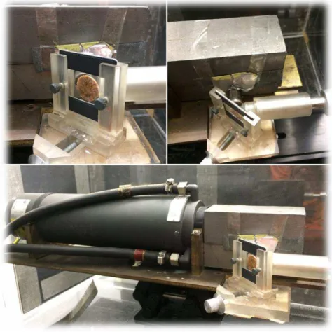
Figure 20 - Position of the sample ready for analysis. Evidence of the tri-axial geometry.

Figure 21 - Sample positioning, moveable stage and M4 TORNADO Spectrometer.

(16)

XVI

Figure 23 - Sample glued to mylar film in photograph slides.

Figure 24 - Sample storage and identification.

Figure 25 - Tri-axial Spectrometer spectrum showed in the adjacent software. Energy value and its counts from each channel are observable.

Figure 26 - TORNADO software presenting the trace element distribution map.

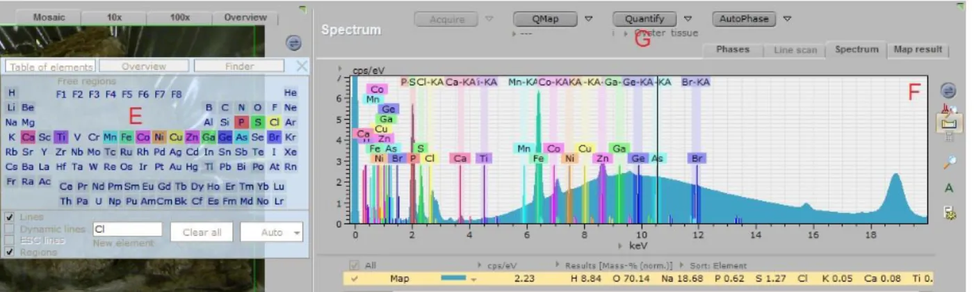
Figure 27 - TORNADO spectrum with trace elements energy peaks and respective identification.

Figure 28 - TORNADO quantification with present trace elements and respective concentrations and associated errors.

Figure 29 – Concentrations from all cancerous and healthy samples obtained from Tri-axial spectrometer.

Figure 30 – Concentrations from all cancerous and healthy samples obtained from TORNADO spectrometer.

Figure 31 – Ca concentrations from each pair obtained from Tri-axial spectrometer.

Figure 32 – Ca concentrations from each pair obtained from TORNADO spectrometer.

Figure 33 – Fe concentrations from each pair obtained from Tri-axial spectrometer.

Figure 34 – Fe concentrations from each pair obtained from TORNADO spectrometer.

Figure 35 – Br concentrations from each pair obtained from TORNADO spectrometer.

Figure 36 – Concentrations from cancerous and healthy bladder tissue samples obtained from Tri-axial spectrometer.

Figure 37 – Concentrations from cancerous and healthy bladder tissue samples obtained from TORNADO spectrometer.

Figure 38 – Br concentrations from each pair of bladder tissues obtained from TORNADO spectrometer.

Figure 39 – As concentrations from each pair of bladder tissues obtained from TORNADO spectrometer.

Figure 40 – Concentrations from cancerous and healthy colon tissue samples obtained from Tri-axial spectrometer.

Figure 41 – Concentrations from cancerous and healthy colon tissue samples obtained from TORNADO spectrometer.

(17)

XVII

Figure 43 – Concentrations from cancerous and healthy lung tissue samples obtained from TORNADO spectrometer.

Figure 44 – Concentrations from cancerous and healthy bladder (1st_{pair) tissue samples obtained from}

Tri-axial spectrometer.

Figure 45 – Concentrations from cancerous and healthy bladder (1st_{pair) tissue samples obtained from}

TORNADO spectrometer.

Figure 46 – Zn concentrations from each measurement of bladder (1st_{pair) tissues obtained from Tri-axial}

spectrometer.

Figure 47 – Concentrations from cancerous and healthy bladder (2nd_{pair) tissue samples obtained from}

Figure 48 – Concentrations from cancerous and healthy bladder (2nd_{pair) tissue samples obtained from}

Figure 49 – Concentrations from cancerous and healthy colon (1st_{pair) tissue samples obtained from}

Figure 50 – Concentrations from cancerous and healthy colon (1st_{pair) tissue samples obtained from}

Figure 51 – Concentrations from cancerous and healthy colon (2nd_{pair) tissue samples obtained from}

Figure 52 – Concentrations from cancerous and healthy colon (2nd_{pair) tissue samples obtained from}

Figure 53 – Concentrations from cancerous and healthy colon (3rd_{pair) tissue samples obtained from}

Figure 54 – Concentrations from cancerous and healthy colon (3rd_{pair) tissue samples obtained from}

Figure 55 – Concentrations from cancerous and healthy lung (1st_{pair) tissue samples obtained from}

Figure 56 – Concentrations from cancerous and healthy lung (1st_{pair) tissue samples obtained from}

Figure 57 – Concentrations from cancerous and healthy lung (2nd_{pair) tissue samples obtained from}

(18)

XVIII

Figure 58 – Concentrations from cancerous and healthy lung (2nd_{pair) tissue samples obtained from}

Figure 59 – Se concentrations from each comparison of cancerous and healthy tissues obtained from Tri-axial spectrometer.

Figure 60–Schematic with the significant trace elements’ tendencies.

Figure 61 – 2nd_{pair of cancerous bladder tissue.}

Figure 62 – Spatial distribution of Ca in the 2nd_{pair of cancerous bladder tissue.}

Figure 63 – Spatial distribution of S in the 2nd_{pair of cancerous bladder tissue.}

Figure 64 – 3rd pair of healthy colon tissue.

Figure 65 – Spatial distribution of P in the 3rd pair of healthy colon tissue.

Figure 66 – 2nd_{pair of healthy lung tissue}

(19)

- 1 -

CHAPTER 1 –

INTRODUCTION

Due to the exponential increase of world cancer incidence and mortality, adding the constant failure to

prevent it, it’s imperative to find new treatments and approach techniques in order to fight this global

epidemic. To be able to counter this disease it is necessary to fully understand its biological and physiological processes. One way to do so is to study the concentration of trace elements present in human tissues. These elements appear in minimal quantities in our cells but they take part in important cell mechanisms, such as cellular growth, by being components of enzymes and catalysts that operate in basic cell chemical reactions. Depending on their concentration, they activate or inhibit certain reactions and

change the membranes’ permeability. In addition, their concentrations vary between healthy and cancerous

tissues in response to this disease’s biological changes. Therefore, by quantifying these elements and

studying their variations it is plausible to observe whether or not the excess or lack of a certain element influences carcinogenesis mechanisms. This will allow the possibility of creating a pattern if these changes are recurrent.

Considering the low concentrations of trace elements in a cell, it is necessary to use a specific technique, such as X-Ray Fluorescence Spectrometry, which allows a multi elemental analysis on trace elements concentration. Some techniques even display their spatial distribution. This technique is based on the interaction between x-rays and matter, in this case, human tissues. The x-rays will excite these tissues and when these return to their normal states they will emit a spectrum of characteristic x-rays that with further analysis will show the specific elements present in that same tissue and their respective concentrations. In this work the chosen XRF technique is EDXRF (Energy Dispersive X-Ray Fluorescence), one of many XRF techniques that highlights the non-destructive method, allowing repeated sample analysis without compromising their composition. The 14 samples of cancerous and healthy tissues, equally divided and paired, will be analyzed through this technique. There are 4 samples from Lung tissue, 4 from Bladder tissue and 6 from Colon tissue. For every cancerous tissue, there is a pair of healthy tissue from the same individual. Unfortunately, the clinical history from each patient was not facilitated, due to bureaucratic problems, which would have helped explaining certain results.

(20)

- 2 -

for example) of cancer and other pathologies, which would help improve early diagnosis measures and new, more efficient, treatments.

This work falls into a series of projects that have as a final objective the ability to perform early diagnosis on cancer and predict its development in the human body. There have been several works previous to this one. The first ones tried to test this spectrometry on biological tissues, being able to quantify each element’s concentration. Others quantified the amount of lead present in human tissues [1]. Then, some works focused on analyzing cancer and healthy human tissues hoping to find correlations in trace element concentration variations but failed to reach a solid one, mainly due to the short number of available samples. This work will try to find more solid conclusions using the same laboratorial environment and techniques but hopefully with more available samples.

In the future, if these correlations are found, it will be able to create a pattern that will make possible the early detection and state evaluation of carcinogenesis by the quantity of each trace element in each cell. So maybe it will finally be at human reach the definite prevention of cancer.

I’ve accepted this work with much esteem because I am closely familiar with a cancer diagnosis and know

(21)

- 3 -

CHAPTER 2 –

STATE OF THE ART

C

ONTEXTUALIZATION

According to 2012 statistics there were diagnosed 14.1 million new cases of cancer worldwide, which represents a significant raise compared to 2008 results. It’s expected that this raise will continue dramatically over the next two decades, resulting in over 20 million new cancer cases. The number of deaths worldwide was about 8 million in 2012. But then again, in the next 20 years this number is expected to rise to 13 million deaths caused by cancer or cancer related problems. Even so, 32.5 million people diagnosed with cancer in the previous 5 years were alive at the end of 2012 [2, 3].

Even though cancer has a worldwide incidence, there are differences in numbers and dominating types of cancer between developed and developing countries. Developed countries show greater incidence in lung, breast, prostate and colon cancer, while in developing countries incidence is higher in stomach, liver, esophagus and cervix cancer. Globally lung and breast cancer have approximately the same number of diagnosed cases, at the top of worldwide incidence. Yet, referring to the number of deaths caused by cancer, lung cancer is responsible for 1.6 million of the 8.2 grand total, much more than breast cancer Although 60% of worldwide cancer incidence is verified in developed countries, more than a half of worldwide deaths were registered in developing countries [4].

(22)

- 4 -

The increasing worldwide cancer incidence will bring even more severe consequences to developing countries, due to the underworld conditions that these populations live in and to the adoption of new and more industrialized lifestyles, such as smoking, alcohol consumption and improper nourishment. Although it is logical to think that in the future cancer will strike harder on developing countries, the enormous costs associated with this disease and population aging confer alarming factors in developed countries. So, to counter this world tendency, it is necessary to improve treatment and early diagnosis measures [5].

Portugal doesn’t escape this tendency and as other developed countries, lung, breast, prostate and colon

cancers are abundant and all in expansion. It is predicted that by 2030, 55 thousand new cancer cases will be diagnosed in that year, which is very alarming [6].

C

ANCER

The ability to improve treatment and diagnosis measures lies on understanding all intervenient factors in the carcinogenesis process, which has several stages and can be originated by genetic alterations or environmental factors. All multicellular organisms’ cells replicate from one mother-cell originating two exactly alike cells. There are mechanisms that ensure this replication is well conducted. If these mechanisms do not work as they should, cells will multiply freely transmitting this characteristic to other cells and forming a mass that is called tumor. There are benign and malignant tumors: the first ones are usually removed with relative ease, however, malignant tumors spread throughout surrounding tissues using bloodstream and the lymphatic system as its transportation, relocating in other parts of the human body, compromising its normal functioning. So, cancer is the term used to designate certain pathologies that present uncontrollable cell growth, therefore including a vast range of malignant masses, differentiated by their origin and severity [7, 8, 9].

Lung cancer has the highest worldwide incidence, resulting in 1.8 million new cases in 2012, that is, 1 in 5 patients diagnosed with cancer, and responsible for 1.6 million deaths that same year. 1 in 13 individuals is expected to developlung cancer in his lifetime, being smoking the ruling factor, causing 22% ofcancer related deaths and 71% of lung cancer related deaths. There are other factors, such as environmental and genetic, assuming a secondary role as smoking turned a worldwide practice of the modern society, traduced in more than a thousand million smokers [4, 10, 11].

(23)

- 5 -

helps protect against this type of cancer. Due to the amount of fat in food, incidence is 20 times higher in developed countries than in developing ones. As prevention, it is recommended to consume less fat and much more fiber [12, 13].

In 2012, 430 thousand new cases of bladder cancer appeared, making it the ninth most common cancer worldwide, responsible for 165 thousand deaths that year. Bladder cancer incidence is more than four times higher in men than women and occur mainly in developed countries. The main causes of this type of cancer are smoking, as in lung cancer, exposure to industrial chemicals and drinking contaminated water, especially water that contains arsenic [13].

(24)

- 6 -

T

RACE ELEMENTS

Carcinogenesis processes are not of easy comprehension, therefore effective treatment is lacking. Even so, new studies have been made, measuring trace element concentrations and analyzing their variations, which could provide core information in helping to understand this disease. Trace elements appear in very low concentrations, inferior to 1000 mg/kg (0.1%), which exist in our body, having the particularity of intervening in important processes, varying their concentrations depending on physical and chemical conditions, as well as physiological and pathological states of the organism. It is plausible to connect their variations with several pathologies’ development [15, 16].

Some of these elements have active roles in carcinogenesis processes, so it’s possible to correlate their

concentrations and ratios with different types of tumors. These elements have their own way of interacting with the human organism, and each have a set of characteristics that can influence or be influenced by carcinogenesis. Some of them are associated with the presence of unpaired electrons that allow their participation in redox reactions [17].

Figure 3– Periodic table with highlighted elements that are essential or are thought to be essential to human organism [18].

Fe (Iron) is an essential element in the human organism due to its role in many physiological functions, certifying that proteins and enzymes work correctly. It is one of the elements that can influence neoplasia development, by intervening in cellular growth and differentiation processes. Studies reveal that Fe present in each cell could promote cancer development as it catalyzes the production of oxygen radicals, which are thought to be carcinogens.

(25)

- 7 -

Cu (Copper) plays an important role in several biochemical reactions inside the human organism. Like Zn, Cu is also a cofactor of superoxide dismutase enzyme, preventing the start and development of tumors. In addition, Cu intervenes in angiogenesis that is indispensable for tumor growth.

Se (Selenium) is accountable for glutathione peroxidases, antioxidant enzymes that protects DNA from free-radicals, therefore related with anti-cancerous effects. Se is thought to be a “redox switch” in the activation or inhibition of cellular growth factors. Its raise promotes cytotoxicity in cancerous cells, altering its metabolism, even though many adjacent processes are yet to be understood [19, 20, 21, 22].

P

REVIOUS STUDIES

As said before, there have already been made several studies in this matter. Some focused on the quantification of trace elements in biological tissues and others tried to find correlations between trace

elements’ concentrations and cancer development.

One of these studies on lung cancer presented some important data regarding element concentration variations and linearity between several elements. For example, P (Phosphorus), Ti (Titanium) and Pb (Lead) concentrations appear to be higher in cancerous tissue, roughly doubling the concentration comparing to healthy tissue. Then, there are many elements that indicate lower concentrations in cancerous tissue: some reduced by half, like Ca (Calcium), Fe, Cu and Zn; and others with greater decrease, like S (Sulfur), K (Potassium), Cr (Chromium), Mn (Manganese), Se and Sr (Strontium). These changes, adding the fact that most of these elements represent great importance in biological and enzymatic processes, establish a pattern in lung cancerous tissues. In fact some of these elements have been under rigorous surveillance since they influence carcinogenesis in laboratory animals. It is thought that nutrients and food components, by their antioxidant characteristics may have an effect in cancer development, accelerating it or stopping it. Furthermore, this study showed linear correlation between certain elements concentrations, for instance, between P and S, Ti and Cr, Mn and Fe, Ti and Se. In addition, Mn and Fe, Se and As (Arsenic) appear to have an antagonist relation [23].

Other data confirm that the most important elements in distinguishing between cancerous and healthy lung

tissues are Fe, Mn and Cu. While for colon the most important elements are Ca, Zn e Fe. This work helped confirm previous studies that indicated that Pb, Cu and Zn concentrations are significantly lower in cancerouslungtissue than in healthy tissue[24].

(26)

- 8 -

and specific food, but none treat the elemental content of food and its relation to this disease. Ca concentrations are very similar in both cancerous and healthy tissues and in some studies its use is suggested as prevention of colon cancer. Low Se levels are thought to be a result of the disease rather than the reason for the tumor development, as so, Se levels should be closely monitored. Se is known for its cancer-protecting effect, however, when in subtoxic concentration, Zn prevents Se activity, accelerating tumor development. Only P, S, K, Ti, Se and Rb (Rubidium) have a tendency to accumulate in cancerous colon tissue [12, 25].

Other studies that are related to colon tissues, verifying that some elements increased their concentrations in cancerous tissues, for example P. These conclusions were reached due to a deeper statistical analysis. Furthermore, the difference in Se concentrations between healthy (higher) and cancerous (lower) tissue may remit to the antioxidant factor of this element, that helps neutralize free radicals [26].

Further studies used and compared two different techniques, EDXRF and TXRF (Total-reflection X-Ray Fluorescence). This study focused on colon cancer showing that Ca and Sr levels are alike in both cancerous and healthy tissues. Moreover, P, K, Cu and Ni (Nickel) were found in higher concentrations in cancerous tissue. On the other hand, Br (Bromine) was decreased in tumor tissue. Zn concentration is either constant or decreased in cancerous tissues. This decrease is also found in other pathologies, for example arteriosclerosis. It can be linked with the alteration of metabolism and modification in the transport and maintenance of essential elements. On the contrary, the increase of some elements can be associated with mechanisms of toxicity whenever these elements are in excess. The results acquired from both techniques are similar, however, TXRF tend to have higher sensitivity for light elements, while EDXRF is more sensitive for heavy elements [27].

More studies related to colon cancer tissues revealed a significant increase in K, Rb and Cu concentrations in cancerous tissues comparing to healthy ones, while Zn and Mn appear to have constant concentrations regarding both types of colon tissues. There is also evidence that Ni and Pb have higher concentrations in tumor tissues [28].

A study with a large number of samples, nearly 14.000, discovered, analyzing iron-binding capacity and transferrin saturation, that high body iron storage elevates the risk of developing cancer. These conclusions were only proved for men, while for women there was no significant data [29].

(27)

- 9 -

tissues belong to specific types of cancer, indicating that analysis cannot group all types of cancer in one class, for interpretation purposes [30].

A work related to patients with bladder cancer studied the concentrations of Cu, Zn, Se, Pb and As. After comparing these elements concentrations the data indicated higher levels of Zn in cancerous tissues than in healthy bladder tissues. This element shows a gradual and significant increase in its concentration as bladder cancer evolves from initial to the advanced stages. The other elements failed to have a statistically difference and so conclusions are undefined [31].

A study that conducted an analysis on breast tissues reached some conclusions. First it showed that trace elements concentrations were higher in tumor tissues, either benign or malignant, than in healthy breast tissues. This, as other previous studies, reveals that trace elements can be used as tumor biomarkers, once they give useful data that allows the distinction between tumor and healthy tissue. It was also found that Cu has a significant correlation with overall survival, meaning that patients with positive expression of this element had poor chances of survival. Other parameters that influence trace elements expression are age and menstrual status [32].

(28)

(29)

- 11 -

CHAPTER 3 –

X-RAY SPECTROMETRY

H

ISTORY

In 1895, Wilhelm Conrad Roentgen accidentally observed in a light-absent room that the radiation from the discharged tubes caused a fluorescent effect on a small black screen painted with barium salts. This was the first time that X-Rays were observed, gaining this denomination because they presented characteristics different from any other kind. These rays are electromagnetic radiation and have wavelengths between 10 -8_{m and 10}-12 _{m and energies between 100 eV and 100 keV. They are produced by the deceleration of}

high-energy particles, through transitions of electrons between atom inner orbitals or by the decay of certain radioactive elements. In the first process X-Rays are emitted in a continuous spectrum, while in the second, as a characteristic spectrum [33, 34].

Figure 4– An electromagnetic wave with a correspondent electric field, magnetic field and direction [35].

Continuous spectrum of radiation occurs when a high-energy charged particle closes in an atomic nucleus, decelerating really fast, emittinga type of radiation called Bremsstrahlung (Brake Radiation). In this interaction, the kinetic energy of the electron is transformed in radiation (photon), posteriorly emitted [36].

(30)

- 12 -

Characteristic spectrum is a result of electron transitions between atom inner shells. If an incident particle or photon interacts with a bound electron of a certain atom, that electron is ejected, creating a vacancy on the atom inner shells. This is called ionization of an atom. Then, an electron from an outer shell transits to occupy the vacancy, originating the emission of a photon through a characteristic spectrum (fluorescence). This photon has the energy equal to the difference between the binding energies of the two shells in question. If an electron is emitted from an outer shell instead of a photon, it is called Auger Effect. The energy of the emitted Auger electron depends on its originating shell [36, 37].

Figure 6– Scheme of X-ray Fluorescence: an electron from the K shell is ejected from the atom due to an incident photon (E0).

Then, an electron from the L shell occupies its vacancy, emitting characteristic X-rays [38].

This characteristic spectrum emission is called X-Ray Fluorescence or XRF and is the main principle of several analysis techniques due to the fact that each element emits a characteristic set of x-rays. The energy of these x-rays is related to the element in question, as the intensity is related to its concentration. The interaction between x-rays and matter was intensely studied, as well as its experimental applications. This was a great help in human organism functional analysis [38].

I

NTERACTION

(31)

- 13 -

Photoelectric Effect happens when a photon or other particle interacts with an inner shell electron of an atom. All the photon’s energy is transferred to the electron, which is ejected with an energy equivalent to the difference between the photon energy and its binding energy to the atom. To occupy the vacancy left by the ejected electron, another electron from an outer shell transits to the lower level of energy, emitting this energy through characteristic radiation. This is the principle of XRF [40].

Figure 7 - Scheme of the Photoelectric Effect and its different stages [35].

Rayleigh scattering or Coherent scattering occurs when a photon interacts with electrons or nucleus, interacting with the atom as a whole. This photon is scattered, maintaining its original energy, but altering its direction. The atom is neither excited nor ionized, hence it is a parametric process. This happens mostly for low energies and high atomic number elements [41, 42].

(32)

- 14 -

Compton Effect or Incoherent scattering takes place when a photon collides with an electron and loses some of its energy, being deflected from its original path. Part of the energy is transferred to the electron. The scattered photon is emitted almost isotropically [43].

Figure 9– Scheme of the Compton Effect [35].

There is also the X-Ray Diffraction phenomenon when a beam of mono-energetic x-rays irradiates a crystal, resulting in a diffracted beam at definite angles, in agreement with Bragg’s law. These last 3 types of interaction increase the detector’s background.

The photoelectric effect and the scattering interactions contribute to the attenuation of x-rays in matter. The Lambert-Beer law shows the reduction of the intensity of an x-ray beam that passes through a certain layer. There are multiple variables in the equation, being the most relevant the mass attenuation coefficient

that depends on the interactions between the beam and the layer, which promotes its attenuation. This coefficient is proportional to the sum of the cross sections for all elementary scattering and absorption process. At the range of XRF energies (< 100 keV), photoelectric effect accounts about 95% of the mass attenuation coefficient, while the scattering interactions comprehend the other 5%. This is due to the fact that photoelectric absorption coefficient is much higher than the sum of the two scattering coefficients [37, 44].

T

ECHNIQUES

(33)

- 15 -

XRF analysis falls into a variety of techniques, being EDXRF(Energy Dispersive X-Ray Fluorescence)

and WDXRF (Wavelength Dispersive X-Ray Fluorescence) the two most used ones. In this work it will be EDXRF the chosen technique to analyze the concentrations of trace elements in all samples. This technique allows a multi-elemental analysis with quantitative and qualitative data of each sample. Inside an EDXRF Spectrometer is a Si(Li) (or similar) detector with high resolution connected to a multichannel analyzer, which allows to obtain a spectrum of x-ray energies. While in a WDXRF Spectrometer is a single crystal placed behind the sample that isolates a narrow wavelength band of the excited sample radiation, through its diffracting power. The main problems with this technique, in comparison to EDXRF, are the fact that only one element can be analyzed at once and that it is extremely time consuming due to its point by point acquisition, rather than EDXRF that acquires the entire spectrum simultaneously [45].

Figure 10 – Difference between EDXRF and WDXRF presented spectrum. Evidence of the EDXRF simultaneous acquisition and the WDXRF point by point one [45].

However, if a more detailed analysis is required, it is recommended the use of an alternative XRF technique, the μXRF (Micro X-Ray Fluorescence). This technique is much similar to the conventional XRF technique, except that it uses X-Ray optics to restrict the excitation beam size or to focus the excitation beam to a small spot on the surface of the sample, in order to analyze its small features [46, 47].

(34)

- 16 -

S

PECTROMETERS

In this work two different EDXRF Spectrometers were used, with many different characteristics. M4 TORNADO from Bruker and a Tri-axial Geometry Spectrometer in-house built. The first one runs a high spatial resolution analysis, recurring to μXRF and returns both an energy spectrum and a map with the spatial distribution of each trace element. The second only returns an energy spectrum with the counts of each energy channel, having the whole sample in consideration.

Commonly EDXRF Spectrometers have a relatively simple composition:  An excitation source (X-Ray tube)

 Focusing optics (μXRF)

 An X-Ray detector with related electronics  A multichannel analyzer

 Dedicated software for rapid, automatic analysis of chemical elements

Figure 12– Simplistic scheme of the M4 TORANDO Spectrometer’s composition [48].

This schematic shows, in a simple way, what happens inside the spectrometer. The Tube emits X-rays that are collimated by the optics and impinge on the sample. Then, the sample emits characteristic X-rays, which are captured by the detector. Further analysis takes place in the adjacent software [38].

(35)

- 17 -

expect good performance from the X-ray tube, some conditions are required: high voltage to analyze all desired elements; specific currents that vary from one spectrometer to another; good stability versus time and appropriate anode material [37].

Figure 13– Simple scheme of an X-ray tube. C – cathode; A – anode; X – Emitted x-rays; U – Applied tension; W – Cooling system (if existent) [48].

The regular EDXRF spectrometer irradiates the sample with X-rays in an area on the order of cm2_{, when}

the sample is homogeneous and sufficiently large. However, if it is small or inhomogeneous the irradiated area must be reduced. If it is desired to reduce it down to an order of 10-4_mm2_{or less,}μXRF_{is required,}

as well as capillary collimators or other kind of X-ray lenses. The most common X-ray lenses can be monocapillary or polycapillary, being the last one the most used in this technique. Polycapillary X-ray optics consist of an array of many small hollow glass tubes formed into a desired shape. They collect the X-rays from the X-ray source with a large solid angle and then redirect them, through multiple internal total reflections, to form a focused or a parallel beam [49].

Figure 14– Polycapillary lens at three different scales [48].

(36)

- 18 -

originating an electronic avalanche and hence a current that is converted into a voltage pulse, by a resistor and a capacitor. Thus, each incoming photon corresponds to an analog voltage pulse, which is then changed to digital by a multichannel analyzer. A detector is characterized by its proportionality, linearity, energy resolution, efficiency and the thickness of its entrance window.

This detector, for laboratory spectrometers, was commonly made of Si(Li), like the one inside the Tri-axial from this work. It consists of a small cylinder of Si with Li to increase its electrical sensitivity. A voltage is applied so Li ions move to a certain layer, which reveals high resistance, forming the depletion area. The incoming photons interact with this area, creating an electric charge proportional to the photon’s energy, which is then processed as mentioned above. Most recently, there was a new development in low energy X-ray detectors through the use of Si monocrystals with the electrode sets arranged in such a way for maximizing charge collection. These new detectors are labeled Silicon Drift Detectors (SDD), and are now almost ubiquitous in any modern EDXRF setup such as the M4 Tornado [50, 51].

Figure 15– Typical Si(Li) x-ray detector, commonly used in EDXRF spectrometers [52].

The final X-ray spectrum presented by the spectrometer contains: a set of lines for each detectable element in the sample, being their energies and intensities dependent on the composition of the sample; a

continuous contribution of the Compton Effect and Rayleigh’s Scattering of incident radiation, depending

on the excitation source and on the sample; lines due to possible “escape” of incident lines in the detector,

depending on the detector and the energies and intensities of the lines; lines due to possible “sum” effects

(37)

- 19 -

Figure 16 – Typical X-ray spectrum obtained with an EDXRF spectrometer [45].

Figure 17– XRF peaks overlapping may happen in the spectrum. Nevertheless, with software calibration the specific XRF peak can be isolated [45].

Data analysis is based in two different relations. First the qualitative relation that has its principles in the Moseley’s Law, which relates the wavelength with the atomic number of the studied element. However the screening coefficient value is required and difficult to obtain, therefore, a database with characteristic transition energies of the elements is consulted by the data analysis code.

This allows the identification of a certain element in a sample by analyzing the energy of the characteristic X-rays emitted by it. The Moseley’s law also helped the ordering of the periodic table, through atomic number rather than atomic weight, as it was previously [54, 55]

(38)

- 20 -

in an energy channel. The more counts, higher intensity and higher the concentration, although no information can be extracted from the relative intensity between elements in the same spectrum [55].

TORNADO

One of the spectrometers used in this work is the M4 TORNADO by Bruker, a μXRF Spectrometer with great speed and accuracy. It allows measurements with information of the composition and element distribution of the sample. It analyzes samples in the solid, liquid or gas state in its vacuum chamber, even if the sample is irregularly shaped. It also presents high element sensitivity and excellent lateral resolution,

up to 25 μm, which allows the mapping of the sample, with the spatial distribution of its composing elements

[56].

M4 TORNADO has a dedicated software, with a great variety of features that allow a deep analysis of the desired sample. In this work, TORNADO will be used to evaluate the spectrum with the energy counts of each element of interest, to calculate the concentrations of those elements in ppm (parts-per-million) and

to observe each element’s distribution in the sample. The operating conditions for all analyzed samples

were 50 kV and 300 mA. The detector is a solid state SDD with an energy resolution of 145 eV [57].

Figure 18– M4 TORNADO Spectrometer manufactured by Bruker and adjacent software [58].

T

RI

-

AXIAL

G

EOMETRY

S

PECTROMETER

(39)

- 21 -

The Tri-axial Spectrometer presents an energy spectrum with the respective counts of each channel. It presents the average concentrations of the whole sample, unlike TORNADO where depending on the chosen area, concentrations can be higher or lower for designated regions of the sample. This allows the identification of the desired trace elements and the measurement of their respective concentrations. The operating conditions were 50 kV and 20 mA and 1000s spectra acquisition [59, 60].

(40)

- 22 -

E

XPERIMENTAL

P

ROCEDURE

The laboratorial work was conducted in Laboratório de Física Atómica e Molecular da Faculdade de Ciências e Tecnologia, at Universidade Nova de Lisboa, being the laboratory supervisor, Professor Maria Luísa Carvalho.

All samples facilitated by Professor João O’Neill from NOVA Medical School were identified with which organ they were extracted from and either they were cancerous or healthy tissues. Then, all samples were submitted to a sample preparation that will be described below. After being prepared, they were repeatedly analyzed in the two different spectrometers. Since a non-destructive technique is used, samples can be analyzed countless times without affecting their compositions.

In the Tri-axial Spectrometer samples were placed in a sample holdernext to the X-ray source and before the detector. Then a 1000 seconds measurement was proceeded, resulting in an energy spectrum that was saved and posteriorly quantified into an excel file with each element’s concentration.

(41)

- 23 -

In the M4 TORNADO samples were placed in the spectrometer’s stage and then placed right below the source and detector. An analysis was then run in an average 5 hour measurement, which resulted in the energy spectrum with peaks from the elements present in the sample and a spatial distribution map, showing where those elements were highly concentrated. The dedicated software allowed the extraction of the desired elements’ concentrations in ppm.

Figure 21– Sample positioning, moveable stage and M4 TORNADO Spectrometer.

With the results from both spectrometers, a further and deeper analysis on the trace elements concentrations and ratios is now possible.

S

AMPLE PREPARATION

(42)

- 24 -

Figure 22– Lyophilizer manufactured by Edwards.

Posteriorly, samples were glued with a specific glue to a mylar film and put in photograph slides which in turn were placed in petri dishes, helping its transportation and storage. Specific glue and mylar film are chosen due to their composition, made only of hydrocarbons, which aren’t detected in XRF, hence not compromising the spectrum for further analysis. Finally, they were numbered and listed by their original organ and whether they were cancerous or healthy tissues.

(43)

- 25 -

A

NALYSIS DETAILS

After a measurement in the Tri-axial Geometry Spectrometer, the energy spectrum is saved both in the computer that is connected to the spectrometer, in order to view it later, and in a personal computer to analyze the containing information. This information is then inserted in a software that makes use of X-ray fundamental parameters and the Sherman equation [55] for calculation of the respective concentrations and associated errors. This raw information has to be treated, eliminating the elements that were below detection levels or those who have great associated errors, which are due to the fact that their concentration is too close to the detection limits. Finally, it is possible to compare trace element concentrations from different organs and different tissues (cancerous or healthy). Three measurements were made for each sample with this spectrometer, in order to improve statistical study.

(44)

- 26 -

Extracting information from the M4 TORNADO is quite different than the Tri-axial. After the measurement is concluded the user is able to see the original sample (A), the distribution of all selected elements in the sample (B) and the separated trace elements’ map with the spatial distribution of each selected element

(C). To observe the correspondent spectrum the user must click in (D):

Figure 26– TORNADO software presenting the trace element distribution map.

The spectrum is then presented. The user must observe the energy peaks in the spectrum in order to identify containing elements and select them in the periodic table (E). The selected elements will appear in colored areas in the spectrum (F) where their energy peaks are known to be, allowing the identification of the present elements. That way the user knows which elements are present in the sample.

(45)

- 27 -

When the user runs the quantify method (G), which is also based on the Sherman equation and the fundamental parameters, only the selected elements are quantified. Both the concentrations and associated errors come in ppm and can be converted into an excel file (H), allowing further statistical analysis. Two measurements were made for each sample with the same objective as stated for the Tri-axial measurements.

Figure 28– TORNADO quantification with present trace elements and respective concentrations and associated errors.

(46)

(47)

- 29 -

CHAPTER 4 –

RESULTS AND DISCUSSION

G

ENERAL CONSIDERATIONS

The number of facilitated samples from NOVA Medical School were not the 20 per organ as expected, for a total of 60; in the end only 14 became available for analysis. These samples were studied by the previously delineated process; this became this work’s biggest obstacle, since the size of the available data is at the core of a reliable statistical analysis. To minimize this issue, repeated measurements were conducted for each sample, 3 with the Tri-axial Spectrometer and 2 with the M4 TORNADO, for a grand total of 70 measurements from 14 samples. From the 14 samples: half are from cancerous tissues and the other half are from healthy tissues; 4 are from bladder tissues, 6 from colon tissues and 4 from lung tissues. Each cancerous tissue sample has a healthy tissue sample pair from the same individual. This allows a more reliable comparison between trace elements concentrations from cancerous and healthy tissues, since when other samples from different individuals are considered, the biological diversity would mask correlations in trace elements concentration variations between similar tissues from different patients. Even so, all samples were studied throughout different parameters and ordered in diverse categories. All analysis obey the general-to-specific methodology. The first analysis includes the results from all available samples. The results are, then, differentiated by their corresponding organs and divided by their pairs, allowing a more specific and reliable analysis.

All the results were listed on an excel file with information on their original organ, the spectrometer utilized, the number of the measurement and whether it is cancerous tissue or healthy. The next step compared the results from cancerous tissues with the results from healthy ones. The results from the two spectrometers were separated due to their different quantification methods and associated errors. Therefore for each comparison there will be two graphs, one associated with the results from the Tri-axial spectrometer and the other with the ones from the TORNADO. Some element concentrations might differ from the two spectrometers due to their different quantification procedures and element detection levels. The concentrations tend to be higher in TORNADO because it runs an analysis on the selected and restricted areas that contain the cancerous part of the tissue. This is important due to the biopsy processes in which the identified cancerous tissue can also include parts consisting of healthy cells. On the contrary, Tri-axial

runs an analysis on the whole sample, presenting the elements’ average concentrations. A detailed

(48)

- 30 -

The concentrations associated errors are represented in each graph’s error bars. When there are several

measurements for the same sample, a single value is required, therefore a weighted average is made. This average and its associated error were calculated with excel’s formulas, based on the general formula of uncertainty propagation, the weighted average being dependent on each measurement’s concentration and its associated error. On the other hand, the weighted average’s combined error depends on the standard deviation and every error from all considered measurements.

The actual concentrations values have no great importance due to diverse factors, such as the different

quantification methods from the two spectrometers, possible laboratorial errors and measurement’s

uncertainty. The main analysis factor is the concentrations variation from one tissue to another, the concentration in cancerous tissues being compared to healthy ones. The graphs are in logarithmic scale in order to allow the observation of all elements concentrations, as they come in different orders of magnitude. This is the observable core of the entire work, on which the desired correlations will be supported.

(49)

- 31 -

G

RAPHIC ANALYSIS

A

LL SAMPLES

Figure 29 – Concentrations from all cancerous and healthy samples obtained from Tri-axial spectrometer.

Figure 30 – Concentrations from all cancerous and healthy samples obtained from TORNADO spectrometer.

P S Cl K Ca Fe Ni Cu Zn As Br Pb

Cancerous 18934.4 6219.88 967.56 1301.13 547.11 951.33 8.79 8.25 70.92 6.66 28.64 4.19 Healthy 14949.4 6674.91 890.42 1148.63 229.91 931.34 12.34 7.08 70.50 6.81 18.26 3.72

1.00 10.00 100.00 1000.00 10000.00 100000.00 Conc e ntra tio n (pp m )

Trace Elements and respective cancerous and healthy concentrations in ppm

All Cancerous vs All Healthy Tissues (Tri-axial)

P S Cl K Ca Ti Mn Fe Cu Zn As Br Sr Pb

Cancerous 7548.2 15806. 3240.2 5681.2 3580.8 8122.7 19.42 3369.6 45.93 466.05 46.13 30.21 3.23 184.16 Healthy 7435.4 15642. 3779.4 6260.5 3196.0 7419.6 21.12 3095.3 46.37 523.13 40.36 60.91 2.95 147.35

Trace Elements and respective cancerous and healthy concentrations in ppm

(50)

- 32 -

These first two graphics have all 14 samples and 70 measurements in consideration, from all organs and pairs. This is the most general analysis of this work. Comparing the obtained results from all cancerous and healthy tissues it is observable that one element increases its concentration, other presents a decrease and the rest maintain their concentrations. Generally the results from the Tri-axial spectrometer are in agreement with the ones from TORNADO, however, there are some observable incoherencies between them. This is also explained by their different quantification methods and detection limits.

Several elements may show a small increase or decrease in their cancerous tissue concentrations, however, a difference is significant and valid only when the error bars do not include the same concentration range. Therefore there are only two elements that almost obey to these conditions. Ca shows higher concentrations in cancerous tissues and Br shows higher concentrations in healthy tissues. The Ca concentration variation is observed in the tri-axial graphic rather than Br variation that is observed in the Tornado graphic. In order to validate these results, the concentrations from each pair of tissues were directly compared, appearing as percentages of the cancerous tissues that show an increase or decrease in their concentrations.

Figure 31 – Ca concentrations from each pair obtained from Tri-axial spectrometer.

Bladder 1st Bladder

2nd Colon 1st Colon 2nd Colon 3rd Lung 1st Lung 2nd

Cancerous 153.48 585.11 929.64 620.43 89.06 477.50 424.24

Healthy 147.73 222.88 194.56 296.27 142.32 234.57 304.73

1.00 10.00 100.00 1000.00

Conc

e

ntra

tio

ns

in

pp

m

Each pair of tissues and respective cancerous and healthy concentrations in ppm

(51)

- 33 -

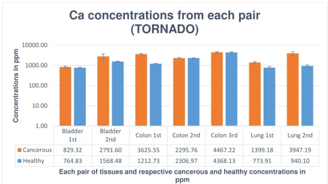
Figure 32 – Ca concentrations from each pair obtained from TORNADO spectrometer.

Thus, it was verified that Ca presented higher concentrations in 86% of all cancerous tissues, observable in the Ca graphics above, in which the concentrations from each pair of tissues are compared.

Figure 33 – Fe concentrations from each pair obtained from Tri-axial spectrometer.

Bladder 1st

Bladder

Cancerous 829.32 2791.60 3625.55 2295.76 4467.22 1399.18 3947.19

Healthy 764.83 1568.48 1212.73 2306.97 4368.13 773.91 940.10

1.00 10.00 100.00 1000.00 10000.00 Conc e ntra tio ns in pp m

Ca concentrations from each pair

(TORNADO)

Bladder 1st

Bladder

Cancerous 641.82 98.75 72.33 158.33 60.00 176.11 1457.14

Healthy 127.00 72.50 55.90 105.94 77.67 290.45 1350.44

1.00 10.00 100.00 1000.00 10000.00 Conc e ntra tio ns in pp m

(52)

- 34 -

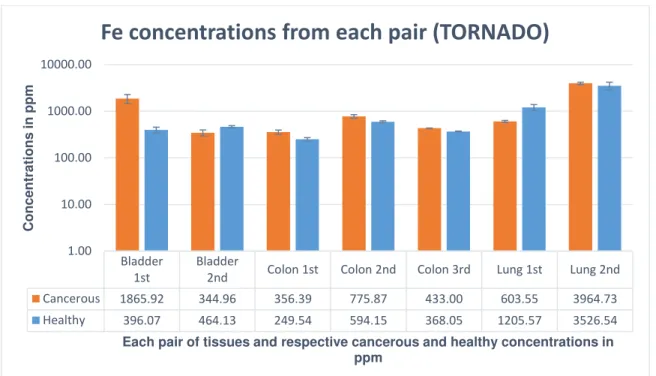
Figure 34 – Fe concentrations from each pair obtained from TORNADO spectrometer.

Although Fe does not show significant differences in its concentrations between cancerous samples, it shows an increase in its concentrations in 71% of the cancerous tissues compared to the correspondent healthy ones. This data is concordant between both spectrometers. This can be explained by the significance of the highest value in the calculation of the weighted average. Even if the majority of the concentrations is higher in cancerous tissues, the weighted average value is similar in both types of tissues, due to the high values of Fe concentration in the 2nd_{pair of lung tissues, which influences the weighted}

average. Biological variability is one of the factors that can mask trace elements concentration variations.

Bladder 1st

Bladder

Cancerous 1865.92 344.96 356.39 775.87 433.00 603.55 3964.73

Healthy 396.07 464.13 249.54 594.15 368.05 1205.57 3526.54

1.00 10.00 100.00 1000.00 10000.00

Conc

e

ntra

tio

ns

in

pp

m

(53)

- 35 -

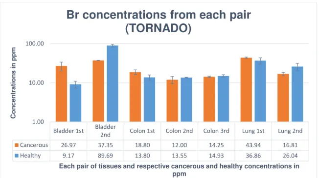
Figure 35 – Br concentrations from each pair obtained from TORNADO spectrometer.

Even though the TORNADO graphic from all samples showed what might be considered an increase in Br healthy tissue concentrations, this graphic that compares each pair of tissue explains that variation. It also discredits this increase due to the fact that almost all concentrations are alike, except the ones from the 2nd

pair of bladder tissues, which presents a great increase in healthy tissue concentration that justifies the variation previously observed.

As so, the most significant elements of this first comparison are Ca and Fe, showing an increase in their concentrations in cancerous tissues of the three types studied, when compared to their healthy counterparts. Past studies stated that excess of Fe present in a cell promotes cancer development [19] and that Br concentration decreases in cancerous tissues [27], while comparing colon cancerous and healthy tissues. There are no more relevant relations with results from previous studies due to the fact that those studies focused on specific organs and not gathering all data, like in this work’s section.

Bladder 1st Bladder

Cancerous 26.97 37.35 18.80 12.00 14.25 43.94 16.81

Healthy 9.17 89.69 13.80 13.55 14.93 36.86 26.04

1.00 10.00 100.00

Conc

e

ntra

tio

ns

in

pp

m

(54)

- 36 -

D

IVIDED BY ORGAN

Having compared cancerous and healthy tissues altogether, one concludes there are not many visible variations and the ones that were noted were not substantiated as wanted. Next, all cancerous and all healthy tissue samples will be divided by their original organ, trying to show trace elements concentration variations in specific organs, what is expected to be easier than with all samples in consideration.

B

LADDER TISSUES

Figure 36 – Concentrations from cancerous and healthy bladder tissue samples obtained from Tri-axial spectrometer.

P S Cl Ca Fe Ni Cu Zn As Br Pb

Cancerous 13730.9 4696.52 436.94 572.86 6.41 7.74 69.52 6.57 34.50 4.06

Healthy 10622.7 5594.22 345.00 194.62 108.83 4.41 7.99 69.17 6.49 21.54 4.14

1.00 10.00 100.00 1000.00 10000.00 100000.00

Conc

e

ntra

tio

n

(pp

m

)

Trace Elements and respective Cancerous and Healthy concentrations in ppm

(55)

- 37 -

Figure 37 – Concentrations from cancerous and healthy bladder tissue samples obtained from TORNADO spectrometer.

These two graphics have all bladder tissues in consideration. There are 4 samples divided in two pairs of bladder tissues. As analyzed before, one can note that some elements increase their concentrations, others present a decrease and many have their concentrations unaltered, when comparing the average values of cancerous and healthy tissue concentrations.

It is easily verified that Ca and Fe appear on average in greater concentrations in cancerous tissues, according to both spectrometers. Other elements show variations in their concentrations according to one of the spectrometers, being unaltered or unseen in the other. For instance, Ni and Ti have higher concentrations in cancerous tissues, while Cl and Br show greater concentrations in healthy tissues. Ni and Cl, the two elements analyzed in Tri-axial may show a variation in their concentrations but analyzing each tissue concentration one observes that the validity of these results is questionable, either due to their very low values or to the fact that it is only observed in one measurement of only one type of tissues. Cl for example is a very good example, as it is superimposed on the Rh L-lines of the TORNADO X-ray tube, and thus were not effectively measured with this spectrometer. A similar effect happens with Sr at the Tri-axial, as the Compton peak from the secondary Mo target masks the K-lines of this element.

P S Ca Ti Mn Fe Cu Zn As Br Sr Pb Si

Cancerous 7559.5 15327. 2519.7 1961.4 22.77 1804.0 50.04 502.35 42.07 32.77 3.58 49.65 15458. Healthy 7567.5 16340. 1374.3 89.71 17.52 433.07 44.07 546.51 41.63 85.26 3.30 25.50 14711.

Trace Elements and respective Cancerous and Healthy concentrations in ppm