BSc in Computer Science

(1)

João Miguel Castanheira Martins

Lightweight Monitoring of Transactional

Memory Programs

Dissertação para obtenção do Grau de Mestre em Engenharia Informática

Orientador :

João M. S. Lourenço,

Prof. Auxiliar, Universidade Nova de Lisboa

Júri:

Presidente: Carlos Augusto Isaac Piló Damásio Universidade Nova de Lisboa

Arguente: Manuel Martins Barata

Instituto Superior de Engenharia de Lisboa

Vogal: João M. S. Lourenço

(2)

(3)

iii

Lightweight Monitoring of Transactional Memory Programs

Copyright c Jo˜ao Miguel Castanheira Martins, Faculdade de Ciˆencias e Tecnologia, Uni-versidade Nova de Lisboa

(4)

(5)

(6)

(7)

Acknowledgements

I am thankful to my adviser, Jo˜ao Louren¸co, for accepting me as his student and also for his guidance, advice, devotion and for being patient with me during the elaboration of the dissertation. I would also like to extend my gratitude to PhD students Ricardo Dias and Tiago Vale for their support when I needed it.

I am grateful to Departamento de Inform´atica, Faculdade de Ciˆencias e Tecnologia, Universidade Nova de Lisboa for granting me with a scholarship during the M.Sc. course. To my co-workers and friends who frequented the room of the Computer Systems Archi-tecture group, for all the moments we shared.

I would like to acknowledge the following institutions for their hosting and financial support: Departamento de Informática and Faculdade de Ciências e Tecnologia of the Universidade Nova de Lisboa; Centro de Informática e Tecnologias da Informa¸cão of the FCT/UNL; and Funda¸cão para a Ciência e Tecnologia in the research project Synergy-VM (PTDC/EIA-EIA/113613/2009).

I also would like to thank my parents for providing me with this opportunity.

(8)

(9)

Abstract

Concurrent programs can take advantage of multi-core architectures. However, writ-ing correct and efficient concurrent programs remains a challengwrit-ing task. Transactional memory eases the task by providing a high-level programming model for concurrent pro-gramming. Still, tools for analyzing and debugging transactional memory programs are very scarce. Tools have been developed for debugging support for transactional memory that rely on logging events (start, commit, etc.) to generate a view of the execution. During the execution, these events are writen to a log, associating a CPU-core dependent timestamp to each event. These clocks are not synchronized and so the events recorded in the log may not respect the real order and appear inconsistent, e.g., thecommit event of a transaction may be recorded as if it happened before the correspondingstart. We present a strategy for ordering the events in a trace log in order to reporduce a consistent view of the events recorded in the log.

Keywords: transactional memory, monitoring, debugging, clock synchronization, event

(10)

(11)

Resumo

Programas concorrentes podem tirar vantagem de arquitecturasmulti-core. Contudo, escrever programas correctos é uma tarefa dif´ıcil. Memória transacional facilita a tarefa, dando ao programador um modelo de programa¸cão de alto n´ıvel para concurrência. Ainda assim, ferramentas para analizar e depurar programas de memória transacionais são muito escassas. Ferramentas de suporte à depura¸cão de programas de memória transacional focam-se no registo de eventos (start, commit, etc.) para gerar uma vista da execu¸cão do programa. Durante a execu¸cão, estes eventos são registados e grava-os numlog, associando

um timestamp dependente do core do CPU. Os relógios não estão sincronizos e, assim,

os eventos registados podem não respeitar a ordem real e podem aparecer inconsistências, e.g., o evento commit de uma transaçcão pode estar registado como se tivesse acontecido antes do evento start correspondente. Apresentamos uma estratégia para reordenar os eventos de modo a gerar uma vista consistente dos eventos registados nolog.

Palavras-chave: memória transactional, monitoriza¸cão, depura¸cão, sincroniza¸cão de

(12)

(13)

List of Figures

1.1 The performance of testing applications with and without the monitoring

system. . . 4

2.1 JTraceView’s workflow. . . 15

2.2 Event log format and example. . . 16

3.1 Description of our strategy’s work-flow. . . 20

3.2 Progression of the TSC core clock in one core. Java benchmark for 5 seconds. 22 3.3 Progression of the system clock vs the TSC core clock, with frequency scal-ing disabled. (Both lines overlap.) . . . 22

3.4 Progression of the system clock vs the TSC core clock, with frequency scal-ing enabled. (The lines almost overlap.) . . . 23

3.5 Linear regression of sample data, with frequency scaling disabled. . . 24

3.6 Linear regression of sample data, with frequency scaling enabled. . . 24

3.7 Merging the logs of three threads into a global log. . . 25

4.1 Execution time for the Intruder benchmark. . . 31

4.2 Execution time for the Vacation benchmark. . . 31

4.3 Abort rate for the Intruder benchmark. . . 32

4.4 Abort rate for the Vacation benchmark. . . 33

4.5 Timestamp inconsistencies for the Intruder benchmark. . . 33

4.6 Timestamp inconsistencies for the Vacation benchmark. . . 34

4.7 Invariant violations for the Intruder benchmark. . . 34

4.8 Invariant violations for the Vacation benchmark. . . 35

4.9 Percentage of out of place events for the Intruder benchmark. . . 35

4.10 Percentage of out of place events for the Vacation benchmark. . . 36

4.11 Late starts for the Intruder benchmark. . . 36

4.12 Late starts for the Vacation benchmark. . . 36

(16)

xvi LIST OF FIGURES

4.14 Premature commits/aborts for the Intruder benchmark. . . 37

4.15 Conflict-free aborts for the Intruder benchmark. . . 38

4.16 Conflict-free aborts for the Vacation benchmark. . . 38

A.1 Timestamp inconsistencies for the Vacation benchmark. . . 43

A.2 Timestamp inconsistencies for the Intruder benchmark. . . 43

A.3 Timestamp inconsistencies for the Labyrinth benchmark. . . 44

A.4 Timestamp inconsistencies for the SSCA2 benchmark. . . 44

A.5 Timestamp inconsistencies for the K-means benchmark. . . 44

A.6 Invariant violations for the Vacation benchmark. . . 45

A.7 Invariant violations for the Intruder benchmark. . . 45

A.8 Invariant violations for the Labyrinth benchmark. . . 46

A.9 Invariant violations for the SSCA2 benchmark. . . 46

A.10 Invariant violations for the K-means benchmark. . . 46

A.11 Out of place events for the Vacation benchmark. . . 47

A.12 Out of place events for the Intruder benchmark. . . 47

A.13 Out of place events for the Labyrinth benchmark. . . 48

A.14 Out of place events for the SSCA2 benchmark. . . 48

A.15 Out of place events for the K-means benchmark. . . 48

A.16 Late starts for the Vacation benchmark. . . 49

A.17 Late starts for the Intruder benchmark. . . 49

A.18 Late starts for the Labyrinth benchmark. . . 50

A.19 Late starts for the SSCA2 benchmark. . . 50

A.20 Late starts for the K-means benchmark. . . 50

A.21 Premature commits/aborts for the Vacation benchmark. . . 51

A.22 Premature commits/aborts for the Intruder benchmark. . . 51

A.23 Premature commits/aborts for the Labyrinth benchmark. . . 52

A.24 Premature commits/aborts for the SSCA2 benchmark. . . 52

A.25 Premature commits/aborts for the K-means benchmark. . . 52

A.26 Conflict-free aborts for the Vacation benchmark. . . 53

A.27 Conflict-free aborts for the Intruder benchmark. . . 53

A.28 Conflict-free aborts for the Labyrinth benchmark. . . 54

A.29 Conflict-free aborts for the SSCA2 benchmark. . . 54

(17)

1

Introduction

1.1 Motivation

The technology of CPUs hit a barrier where the economic effort of producing CPUs by increasing their clock frequency was no longer viable. While it was technologically possible to increase CPU performance by simply increasing its frequency, it is economically unfea-sible to do so due to concerns such as heat losses and power consumption. Multi-core and multi-processor architectures address this barrier by, instead of developing faster CPUs, shifting the focus towards aggregating a set of CPUs in a single chip, and letting the Oper-ating System (OS) distribute the workload among them. Multi-core architectures became the standard for both personal and industry machines. This paradigm shift in hardware imposes a paradigm shift in software development, from sequential programming to par-allel programming.

(18)

1. INTRODUCTION 1.2. Non-intrusive Program Monitoring

threads can lead to a very different behavior and result. Debugging tools for concurrent programming were developed to tackle the issues above.

Transactional memory (TM) was proposed as higher level paradigm for concurrent programming than other lower level mechanisms, such as the usage of threads with locks. This paradigm allows a set of operations (transactions) to execute atomically. Neverthe-less, these are still affected by performance and correction errors. Concurrent programming remains a difficult task. To identify, diagnose and correct the errors in concurrent pro-grams, it is possible to monitor the behavior of programs during their runtime, logging the relevant events and analyzing those logs to gather statistical information and behavior patterns that will help in identifying the observed error.

1.2 Non-intrusive Program Monitoring

Program monitoring relies on performing trace function calls to log certain relevant events during the execution. The events logged are put into a trace file that represents the time--line of the program. Due to the overhead introduced by the tracing calls, the behavior of a monitored program execution may differ from a non-monitored one. For instance, the execution of a monitored TM program may have an abort rate of 90%. However, when it is monitored, that rate may drop to 10%, on account of the tracing intrusion. As a general case it is acceptable for program to run slower, while being monitored, as long as it shows the same behavioral pattern of a non-monitored execution. To trace the behavior of a TM program, it is necessary to register the transactional events (start, commit, etc.), with an associated timestamp, so the events can be consistently mapped to the time-line of the program. When a global clock is used, the access to read the clock value becomes a bottleneck in the system, as it forces the various threads to synchronize. As such, a global clock makes the tracing system intrusive and is not a viable option when dealing with such low level operations such as memory accesses.

One way to address this issue is to use local clocks. If every thread reads from its own clock then there is no need for a synchronization mechanism. This makes the use of local clocks a viable alternative. However, local clocks are not synchronized and this may lead to an inconsistent trace file. For example, a thread may start executing in core 1 and perform a few operations, then migrate to core 2 and perform the rest of its operations. It may happen that core 2’s clock has a smaller value than core 1’s clock. In this case, the instructions performed in core 2 would appear as having been executed before the ones executed in core 1. If we want to achieve a consistent log, we must synchronize the clock values. To minimize intrusion, this correction should be done off-line. The offset of the clock values is not always the same as they usually grow further apart as time passes. This phenomenon is called clock drift. Clock drift represents the speed at which a clock moves away from a reference clock.

(19)

1. INTRODUCTION 1.3. Context

perform slower at lower CPU frequencies and faster at higher frequencies. The program will sometimes run faster and sometimes run slower, when the frequency is varying. This makes the CPU behavior unpredictable and becomes impossible to reproduce a similar behavior. Monitoring programs with frequency scaling enabled is a problem outside the scope of this work.

1.3 Context

To trace a transactional memory program, we register information about transactional events (start, commit, abort, reads and writes) that occur during runtime, together with a timestamp so that we can order the events. We may collect the timestamp by recurring to a global clock, for instance an atomic counter. However, this introduces additional synchronization in the program and alters its behavior. A more viable strategy is to use local clocks, like the register counters available on each CPU core (e.g., the RDTSC in Intel/AMD CPUs), which will minimize the impact in the program behavior.

Figure 1.1 shows a comparison between the behavior of non-monitored and monitored execution of transactional memory programs. The left column refers to a Linked List benchmark and the right column refers to a Red-Black Tree benchmark. The green (or light grey) lines represent the executions in read dominant environments and the red (or dark grey) lines represent executions in write dominant environments. The first row shows the behavior of the benchmarks running without monitoring, establishing the expected runtime behavior of the programs. The second row shows the behavior of a monitored execution of the same benchmarks using a Single Atomic Counter (SAC) as a global clock. When using this type of clock, we can see that the behavior of the programs can change radically, specifically, the synchronization added by using an atomic counter becomes a bottleneck in the system and it no longer scales as before. This shows that the usage of a global clock for monitoring the events of programs is intrusive, making it an unfeasible solution. The third row shows the execution of the linked list and red black tree benchmarks using the Time Stamp Counter (TSC), a clock register available on each CPU core, as the local clock for collecting timestamps. Contrary to the second row, the behavior of these executions remains similar to the original unmonitored behavior. It is noticeable that the programs run slower, since they execute less operations per second; however, this slowdown is not a problem because it is still possible to reproduce a behavior that is similar to an expected ”real world” execution of the program. This shows that the TSC core clocks can be used as a non-intrusive alternative to the SAC global clock. However, the TSC clocks are local to each CPU core (and linked to the clock frequency) and, as such, the clocks are not synchronized which lead to problems when trying to extract debug information from trace logs. Different timestamp values might be read from different clocks at the same time, and as time passes the offset between their values may increase causing even more inconsistencies in the trace log.

(20)

1. INTRODUCTION 1.3. Context 0 50 100 150 200 250 300

1 2 4 8

1000x

Operatio

ns/second

Number of threads List 1000 nodes

5% insert, 5% remove, 90% lookup 45% insert, 45% remove, 10% lookup

0 1000 2000 3000 4000 5000 6000

1 2 4 8

1000x

Operatio

ns/second

Number of threads Red-Black 1000 nodes

0 5 10 15 20 25

1 2 4 8

1000x

Operatio

ns/second

Number of threads List / Atomic Counter / 1000 nodes

0 50 100 150 200 250 300 350

1 2 4 8

1000x

Operatio

ns/second

Number of threads

Red-Black / Atomic Counter / 1000 nodes

0 20 40 60 80 100 120

1 2 4 8

1000x

Operatio

ns/second

Number of threads List / RDTSC Counter / 1000 nodes

0 500 1000 1500 2000 2500

1 2 4 8

1000x

Operatio

ns/second

Number of threads

Red-Black / RDTSC Counter / 1000 nodes

(21)

1. INTRODUCTION 1.4. Log Inconsistencies

transaction may start executing in CPU core 1 and then migrate to CPU core 2 where it ends its execution. If the timestamps collected in core 2 have earlier values than the ones collected in core 1, then the trace log will show the events in core 2 recorded before the events recorded in core 1. From the trace log’s perspective, that transaction performed some operations before it started and so it is an inconsistent trace log.

1.4 Log Inconsistencies

Due to clock drift among the TSC core clocks, the registered events during the program runtime may be out of order and the generated log may contain inconsistencies. The events of a given thread from the log might not show the correct ordering according to their timestamps, i.e., a later event might have a smaller timestamp than a previous event. However, if the logs’ timestamp appear to give a correct ordering of the events, it is still possible that some events are out of order, e.g. a log may show that a transaction did a read operation immediately before the start operation. This can be detected by verifying that the recorded operations in the log respect the transaction constructs. As such, in-consistencies can be categorized in two types of inin-consistencies: temporal inin-consistencies and operational inconsistencies.

Temporal inconsistencies Temporal inconsistencies refer to the ordering of the events

in the log. They exist when there is an error in the log’s sequence of events, due to core migration. These inconsistencies are not related to transactional memory and can be used in a general setting for ordering any sort of events. Nevertheless, they only reveal the most obvious errors in logs and correcting them does not imply that the log is correct. There can be two types of temporal mistakes: jumps backward and jumps forward in time. Jumps back in time are easy to detect in a trace file sorted by operation order. If event

ei has timestamp that is greater or equal that ei+1’s, then time appears to have stopped

or gone backwards and we have an inconsistency. However,ei+1 might have a timestamp

much greater thanei’s and it is hard to detect this as an inconsistency because time kept going forward. The events afterei+1 may have lower timestamps thaneiand we can detect

these jumps back in time. Nevertheless, we will not detect the inconsistency between ei

and ei+1.

Operational inconsistencies Semantic inconsistencies point out other kinds of errors

(22)

1. INTRODUCTION 1.5. Contributions

This work focuses on studying the relation of the TSC (Time Stamp Counter) core clocks and the system clock and apply the knowledge about their offsets to correct the errors in trace logs of transactional memory programs.

1.5 Contributions

This work contains the following contributions:

• A study of the relation between the system clock and the distributed core clocks;

• An off-line clock synchronization strategy and its implementation;

• Implementation of programs to verify the consistency of transactional logs;

• Experimental evaluation of the proposed strategy;

• A software prototype that is available to the scientific community.

1.6 Outline

(23)

2

Related Work

This chapter will provide an overview of the existing related work. Section 2.1 provides an overview of transactional memory and the most important work and definitions developed. Section 2.2 provides classifications for clock synchronization approaches and presents the methods from the literature. Section 2.4 provides a summary of the trace generation techniques developed so far. Section 2.5 presents the framework developed that is the motivation of this work.

2.1 Transactional Memory

The advent of multi-core and multi-processor architectures has increased the need for better parallel programming models. We can classify two forms of parallelism: data paral-lelism and task paralparal-lelism. Data paralparal-lelism is a programming model where one operation is executed over a set of data. Certain languages, like High Performance Fortran, imple-ment this kind of parallelism. It is useful, for example, for computations over matrices. Since the parallelism is usually implicit, synchronization and load balancing are delegated to the compiler or the runtime system. Task parallelism is a programming model where several operations are executed on different threads. In this model, the coordination is explicit via fork-join operations, locks, semaphores, etc. While task parallelism is powerful and a general way of expressing parallelism, it is a low level abstraction which makes it difficult to work with.

Transactional memory (TM) [Her+93] tackles these issues by providing a high level interface to the programmer to perform task parallelism. A transaction is limited by

a start operation and a commit operation. In between these operations there is code,

(24)

2. RELATEDWORK 2.1. Transactional Memory

by the transaction is called the read-set. The set of variables that the transaction writes on is called the write-set. Semantically, a transaction either executes its entire code, i.e. it commits, or none of it, i.e. it aborts (as if it never executed). The commit operation ensures this behavior. Many TM systems also provide an abortoperation that explicitly aborts the transaction. This leads a useful abstraction known as the atomic block. An atomic block is a programming language construct that wraps a sequence of statements in betweenstartandcommitoperations. Reading and writing to variables is also performed with the semantics described above. Thus the programmer’s task is simplified to deciding which parts of the code should execute atomically, i.e., are enclosed in atomic blocks. Transactions provide a useful abstraction for concurrency. They were initially used in databases. A database transaction has four properties, know as the ACID properties, that carry onto transactional memory:

• Atomicity - all actions in a transaction complete successfully, or none of them appear to have executed;

• Consistency - transactions do not violate application specific invariants;

• Isolation - running transactions do not interfere with each other;

• Durability - once a transaction commits, all subsequent transactions should see the committed transaction’s effect.

(25)

2. RELATEDWORK 2.2. Clock Synchronization

it allows us to make a copy of the state (a snapshot), perform the transaction on that copy, and at commit the (modified) snapshot is written to memory. It also allows differ-ent transactions to execute on iddiffer-entical snapshots and then commit the differdiffer-ent sets of updates. However, this may lead to inconsistencies in the memory.

During runtime, if transactions are allowed to interfere with each other, causing a conflict, they would produce undesirable results that violate the semantics of transactional memory. For example, when two different transactions try to write on the same variable, or when one transaction reads a variable while another transaction is writing on it, a conflict occurs. A conflict can be detected eagerly or lazily. The first strategy detects conflicts when two (or more) transactions access the same memory zone and one of the accesses is a write. Conversely, in the lazy scheme conflict detection is delayed until transactions attempt to commit. When a conflict is detected it can be resolved immediately (for example, by delaying one conflicting thread) or it can be resolved during the commit by a contention manager. The contention manager chooses which transactions commit and which abort (or are delayed) in a way that there is no interference between transactions. There are many different strategies a contention manager can employ [Gue+05a; Gue+05b; SI+04; Sch+05]. The simplest can abort and re-execute the transaction or it can delay the transaction using an exponential backoff. Some more complex strategies assign a weight or a priority to each transaction and then use these values to decide which transactions commit. The most complex strategies are usually a combination of simpler strategies, such as the ones above. In order to manage the tentative writes a transaction performs two strategies can be employed. One way to tackle this problem is letting the transaction write to the memory directly and keep an undo-log in case it gets aborted. The other way is to perform the writes on buffers and only write them to memory when the transaction commits. Other problems can occur [Shp+07], specially when combining transactional and non-transactional code. A transaction may read multiple times from a variable and in between those reads non-transactional code may write a new value to that variable. Unless the old value is cached this update will be seen in the transaction. A worse scenario is if that write was in between transactional reads and writes. This way, the non-transactional update would be lost. In TM systems that use an undo log, non-transactional code may read from a value form a variable that was written by a transaction that was eventually aborted.

2.2 Clock Synchronization

(26)

establishes a total order of events. There are two ways of achieving clock synchronization: external and internal.

In external clock synchronization, there is an external time reference and the clocks synchronize themselves with that reference. This type of synchronization relies on the time reference that is responsible for ensuring the correctness of the synchronization. If the time reference fails, it is not possible to synchronize the clocks. NTP [Mil89] is a protocol widely used in the Internet to synchronize clocks. It uses a set of time servers (a replicated time reference) and, for example, the personal computers communicate with the time servers to synchronize their clocks. The time servers themselves are divided into a hierarchy. At the top the servers with the most precise clocks and at the bottom the ones with the least precise. Servers in one layer synchronize themselves with the ones in the above layer. Cristian [Cri89] presents an algorithm that uses a two types of servers: masters and slaves. The masters serve as an external time reference and the slaves synchronize themselves with the masters.

In internal clock synchronization, clocks read each others’ values and compute, or estimate, an error bound on that reading. This removes the need for a time reference (that may fail) but adds the weight of performing more operations on each node to synchronize the clocks. An example of this form of synchronization was presented by Lamport [Lam78]. The algorithm synchronizes the clocks of a distributed system by sending timestamped messages. When a message arrives at a node, it sets its clock to the maximum of its current value and the increment of the message timestamp, i.e. if a node has its clock with value c and receives a message with timestamp t, it sets its clock to max(c, t+ 1). This also ensures that every node sees the messages being received after they are sent. Google’s Spanner [Cor+12] uses Marzullo’s algorithm [Mar+85] to synchronize clocks across geographically distributed data centers. Given a set of measurements and their uncertainty, the algorithm ensures that it finds the interval that is consistent with the other measurements or with most measurements.

Most of the research developed has been in the context of distributed systems. There are many issues when trying to implement clock synchronization in a distributed system. In order for the processes to synchronize their clocks, they have to communicate with each other. This can become a bottleneck, specially if there is a synchronization phase which will flood the network with timestamped messages. Additionally, the round trip time of the messages must be taken into account. When a processP sends a timestamped message to another process Q,P’s clock will be greater or equal to the timestamp in the message, when it arrives atQ. In a distributed system, processes can have different types of failures, such as fail-stop, crash or byzantine. These must be taken into account when designing a clock synchronization algorithm for a distributed system.

(27)

will be processed and from which the timeline will be rebuilt. This is called offline clock synchronization.

2.2.1 Online Clock Synchronization

To synchronize clocks at runtime, the system must perform additional actions, such as reading remote clocks, computing error bounds, performing a synchronization phase, etc. This added effort can become a bottleneck for the system. For example, during a syn-chronization phase in a distributed system, the processes must communicate with each other and synchronize their clocks. This can lead to a quadratic exchange of messages, coming in a burst, causing poor performance during the synchronization phase. Lamport timestamps [Lam78] and the Network Time Protocol [Mil89] are both examples of online clock synchronization.

One way to synchronize the clocks is to synchronize their time and their frequency, preventing clock drift. In order to do this, Dunigan [Dun92] estimates the offset and skew of different processor cores in a hypercube machine.

Another way of achieving this is to chose one processor as a time base, and have the remaining processors synchronize themselves with it. In [Mai+95], each processor estimates the offset and drift with relation to the time base. This estimation is done in rounds where transputers in a cluster communicate via messages between them, using RTT measurements. Timestamps are collected at the sending and receiving of messages on both processors. From this data, and taking into account the message transmission delay, the offset and drift are computed.

Probabilistic clock synchronization [Cri89; Cri+94] is an approach that does not ensure correct results, but achieves them with high probability. When successful, algorithms for probabilistic clock synchronization achieve higher precision and better performance than deterministic algorithms. The downside is the possibility of failing to read the correct clock value.

The more precise the synchronization needs to be, the more measurements it will have to take, and thus, this will result in worse performance. With less measurements better performance is achieved, but there is a greater chance a wrong value was read. However, there is a strict limit on the number of possible measurements taken, so it won’t read clock values ad infinitum. Some of the measurements might also be discarded because they do not comply with correctness requirements. This happens when a measurement takes too long because of a sudden unexpected burst in the network.

(28)

process won’t try to read ad infinitum. The method presented in [Cri89] generalizes clock synchronization algorithms as it behaves deterministically, given the precision required is high enough. This method was further improved [Cri+94], where it was adapted so it performs internal clock synchronization. Each process runs a time server, and exchanges messages with other processes. A family of algorithms is presented [Cri+94], each tol-erating a different class of failures. The algorithms use a linear number of messages to synchronize the clocks.

2.2.2 Offline Clock Synchronization

Offline clock synchronization algorithms work by reconstructing the execution timeline, during post-processing. During execution, timestamps, and additional relevant informa-tion, are collected when events occur. Reading the timestamps must be a lightweight operation, as it should not become a bottleneck. After the execution, the collected in-formation is processed, for example, computing the offsets and drift between the clocks. After processing all information, it should be possible to have a global timeline of the events, which can be very useful for establishing their total order.

Offline clock synchronization is useful for program debugging. An execution of a pro-gram with the time information being collected should have the same behavior as when it executes without collecting the time information. This does not necessarily mean that both executions should have similar execution times. An execution with time collection may run slower than one without, as long as it runs slower at a constant rate, i.e. the program suffers from the same slowdown at all times.

To avoid intruding in the program execution, timestamps can be taken at relevant events of the program. This is done in [Wu+00], for massively parallel computers, where local timestamps are collected at each event occurrence. It also periodically takes a local and global timestamp pair on each CPU core. With this information it is possible to compute the offset and drift of each clock with respect to the global clock, and thus compute the global timestamps of the events.

Gottschlich et al. [Got+12] present a transactional memory tracer that collects times-tamps when a thread enters and leaves a CPU core and on the start, commit and abort of transactions. Their framework collects local clock timestamps for lightweight transactions and global clock timestamps for heavier transactions. They also monitor the beginning and ending of threads but not the memory accesses performed.

(29)

2. RELATEDWORK 2.3. Time Stamp Counter

2.3 Time Stamp Counter

Collecting timestamps is important for benchmarking, as it allows the reconstruction of the events’ timeline. However, reading from the global system clock is a heavy operation that would make timestamp collection intrusive. To cope with this, processors have a time stamp counter on each core.

The time stamp counter is a 64 bit MSR (model specific register) that is incremented every clock cycle. On reset, the time stamp counter is set to zero. It counts the number of cycles that have elapsed until it was read, if we wish to convert it into time we can use the following formula:

seconds = cycles frequency

In order to read from the time stamp counter, processors have two instructions available:

rdtscand rdtscp.

The rdtscinstruction stores the 64 bit unsigned timestamp asEDX:EAX, i.e. the

high-order 32 bits of the timestamp are stored in the EDX register and and the low-order 32 bits into theEAXregister. One can recover the timestamp by reading from theEDXvalue, shifting the valueEDXby 32 bits, and then applying a bitwiseORoperation with the value read from theEAXregister.

timestamp= (EDX<<32)|EAX

For Intel 64 processors, the high-order bits of RDXand RAXare cleared.

In order to avoid wasting CPU clock cycles, instructions may be executed in a different order than the one from the source code. This could be a problem when using the rdtsc

instruction, as it could be executed at a different time than it was expected to and provide unreliable results. For example, if we want to know the time it takes for a certain operation to complete we would place it between two rdtsc instructions. Out of order execution might run the two rdtsc in sequence before the heavy operation. The result would be that the heavy operation is very cheap, when in fact it is the opposite. To prevent such erratic behavior, a serializing operation is required.

The cpuidis a serializing instruction that ensures that, when it is executed, the code

above it has finished executing and the code below it has not yet started executing [Gab10]. It also writes processor information to the registers. According to [Int97], the best way to measure the cost of a cpuid instruction is to call it three times and use the third measurement.

(30)

2. RELATEDWORK 2.4. Trace Generation

RCXare cleared. Therdtscp is a serializing variant of therdtscwhich ensures that, when it is executed, instructions above it have finished their execution. However, instructions below it may have already started executing due to out of order execution [Gab10]. To see if the rdtscpinstruction is available on the CPU, rdtscpmust be set in the CPU’s flags. For instance in Linux, do a cat /proc/cpuinfoand see if rdtscp is one of the flags.

Another possible behavior that may cause incorrect result is counter overflow. This would occur if the measurements took longer than 264 _{cycles. For a 1 GHz CPU, this}

would mean that the code would run longer than:

264

109 = 18446744073 seconds≈585 years

Considering that our main focus is program debugging, counter overflow shouldn’t be a problem because tracing shouldn’t take more than a few hours at most.

2.4 Trace Generation

When using debugging tools, it is often useful to collect information at runtime to later analyze and determine the behavior of a program. Collecting data at runtime will make the program run slower, however, this is not a problem if every step of the program is slowed down by the same amount. If the tracing slows down different steps by different amounts, the tracing becomes intrusive. This means that the program behavior will not be the same than when running without the tracer. In the end, the debugging information collected will be from a different execution than the real world ones, with different interleavings between threads and transaction throughput. Thus, the data collected will not yield significant improvements for the program, since it comes from an execution that does not show the behavior of an unmonitored (and real world) execution. On one hand, the more data collected during runtime, the more information we can extract during the analysis. On the other hand, the more data collected, the longer the trace generation will take. This will likely make the trace generation more intrusive.

(31)

2. RELATEDWORK 2.5. JTraceView

are accessed by a second set of threads that compress the information and write it to disk. Multiple files are written as to avoid synchronization mechanism that would induce delays. A different approach was proposed by Gottschlich et al. [Got+12]. Each thread stores the log information in its local storage, and when it terminates compresses and writes the log to the disk. Again separate files are used to avoid synchronization. This work further reduces the intrusion by not logging the writes and reads. Instead, the contention manager writes the abort reason on the transaction, when it is aborted, to compensate for some information loss that could be provided by logging the reads and writes. Wu et al. [Wu+00] developed a trace analysis framework for MPI. The threads running the MPI calls collect the log data and write it to a file. Multiple files are generated that are later merged.

By providing a programmer API, it is possible to choose which transactions are logged, at the cost of having to place the framework calls manually. The calls store information in separate buffers and they are written into a single log file on application termination. By logging reads and writes of shared resources the intrusion is increased a bit, but the information retrieved can help infer useful information, like finding which transaction was conflicting with another transaction that aborted. The events logged are kept in main memory, using a representation that ensures a small memory footprint.

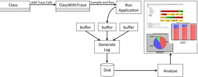
2.5 JTraceView

This section provides an overview of JTraceView [Lou+09], the monitoring tool for trans-actional memory programs that this builds upon. The framework logs the start, the commit or abort, and every read and write to a shared memory location in a transaction. Specific tracing calls must be added to the source code in order to perform tracing. The tracing component records events during the program runtime and generates the log when the execution terminates. The visualizer component then analyzes this log and presents a graphical representation of the information. JTraceView’s workflow can be seen in Fig-ure 2.1.

Analyse( Generate(

Log(

buﬀer( buﬀer(

buﬀer(

Disk(

Run( Applica8on( ClassWithTrace(

Class( Add(Trace(Calls( Compile(and(Run(

Individual Transaction Percentages

Code 0Code 1Code 2 Code 2 10%

Code 1 45%

Code 0 45%

Read/Write Transaction Rates

ReadWrite Code 0 Code 1 Code 2

Individual Transactions 0

10 20 30 40 50 60 70 80 90 100

%

74.435 25.565

85.455 14.545

100

(32)

There are seven different event types: TxStart, TxRead, TxWrite, TxCommit, Tx-AbortUser, TxAbortCommit and TxAbortOther. The structure of a logged event is as follows:

• timestamp - The time instant in which the event occurred;

• eventId - The identifier for the type of the event (TxStart, TxRead, etc.);

• threadId- The identifier of thread executing the event;

• transactionId - The identifier of the transaction in which the event occurred.

For the TxRead and TxWrite events, the memory location address is also logged. Each thread keeps the logged events in a private buffer in a compact binary format. This ensures the framework has a small memory footprint. It also allows threads to work independently as to not introduce synchronization between threads. When the application finishes executing, the events in the buffer are merged into a single text file. See Figure 2.2 for an example log. By having the threads execute independently and only writing the information to disk at the end of the execution, the tracing performed is not intrusive and maintains the global application behavior.

Figure 2.2: Event log format and example.

The framework provides a visualization tool that presents statistical information in the form of charts and shows the transactional computations across a timeline. This information is generated from the logs. However, these logs can be very large in size and may not be loaded into memory. Instead, they are viewed as a list of events using a sliding window to read a limited amount of information from the file. The visualization tool supports, so far, ten different types of charts:

• Abort Types - Shows the percentage of aborts per type. Helps understand the

eagerness of conflict detection.

• Commit/Abort - Percentage of committed transactions vs aborted transactions.

Shows wasted work.

• Transaction ID - Distribution of user-level transactions. Represents application

(33)

• Read/Write Rates- Percentage of read and write operations performed per

trans-action. Further help in understand application behavior.

• Commit/Aborts XY Chart- Percentage of committed and aborted transactions

across execution time slices. Shows throughput along the execution.

• AccessMemChart- Shows memory position access rate. Helps identify contention

points.

• Transaction Retry Rate- Shows average number of retries per user-level

trans-actional operation. Helps understand contention of each operation.

• Transaction Duration- Shows the minimum, maximum and average duration, in

logical time, of transactions. Helps understand the uniformity (or lack of) of the work done by transactional operations.

• Abort Reason- Shows percentage of transactions that were aborted by false

con-flicts. Allows to understand if the contention policies of the underlaying TM are adequate for the transaction.

• Retry Rate - Shows the wasted and useful work distribution. Helps understand

the usefulness of the underlaying TM.

(34)

(35)

3

TMTracer - A Lightweight Library

for Java Programs

This chapter provides a detailed description of our proposal of a lightweight tracing library for Java programs. Clock synchronization is a classic problem from distributed systems. Generally, the proposed strategies to address this problem rely on the temporal order relation of sending and receiving messages and round trip time estimates to adjust the values of the clocks [Lam78; Mil89]. However, that is not the case for multiprocessor systems, where there is no message passing and the read/write operations do not share a temporal ordering. Another issue is that clock error tolerance is greater in the distributed systems context, since memory accesses are much faster than message passing.

3.1 Approach

(36)

3. TMTRACER- A LIGHTWEIGHTLIBRARY FORJAVAPROGRAMS 3.2. Estimating the clock drift

synchronization is addressed by estimating the clock drift and knowing the initial offsets of the clocks with respect to a time reference. Before and after the program is run, we perform a sampling phase on the machine to estimate the clock drift of each core clock against the time reference (i.e., the system clock).

Sampling

Phase 1 Run Program

Sampling Phase 2

Sampling

Data 1 Event Log

Sampling Data 2

Run Correcion

Corrected Log

Figure 3.1: Description of our strategy’s work-flow.

3.2 Estimating the clock drift

While logging the transactional events, it is important that the timestamps are accurate and precise to simplify the process of ordering the events by correcting the measured times. The collection of the timestamps must also be a lightweight operation, in order to avoid impacting the program runtime behavior. If the operation is intrusive, then the program will spend a significant amount of its runtime doing time measurements rather than the original operations and the behavior will change.

To measure the core clock values with precision we use the Time Stamp Counter (TSC) register. The TSC register is a 64 bit unsigned register that is incremented every clock cycle and resets on power on. We use therdtscpinstruction, which reads the 64 unsigned bit value of the Time Stamp Counter register and loads its 32 high order bits into EDX

(37)

Initially, we perform a sampling phase to estimate the drift between each core clock and the system clock. We use this information to correct the event timestamps, which contain core clock measurements. The sampling phase runs by taking several core clock and system clock measurements to establish a parallel progression. Since both operations can’t be performed at the same time, we take two measurements of the core clock (because it is lighter) and one system clock measurement in between. We use the system clock as a time reference because we cannot measure the value of two cores at the same time, since there is no way to reliably force an operation to execute on a core. We consider the midpoint of the two core clocks to represent the same time as the system clock measurement. We also perform dummy work after the three measurements to keep the CPU cores busy, and measure again. This repeats for a configurable amount of time and executes on every core of the CPU (one thread per CPU core).

During the monitored execution, the tracing system uses the TSC to register times-tamps with the logged transactional events. Using the set of core-system timestamp pairs acquired in the sampling phase, we use a linear regression to construct, for each core i, a function of the form fi(t) = δit+θi, whereδi is the drift rate of core i form the system clock, and θi is the initial offset of corei to the system clock. Each timestamp ti, taken in corei, is then corrected by replacing it with fi(ti).

We implemented the sampling phase specification, in Java, and used it as a benchmark to study the clock drift of eahc core clock with respect to the system clock. We use the

rdtscp instruction to read the TSC clock value as well as the core id. We wrap the call

to the assembly instruction using the Java Native Interface (JNI). The benchmark was executed on a Sun Fire x4600 machine described in Table 3.1.

Table 3.1: Machine specifications

Model Sun Fire x4600 Processors 8 dual-core AMD @ 2.7 GHz

Cores 16

RAM 32 GB

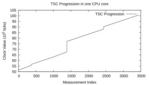
The benchmark results showed that the clock drift is linear during segments of time, as seen on Figure 3.2. However, sometimes there are time jumps and the read value is much higher than the previous one.

(38)

50 55 60 65 70 75 80 85 90 95 100 105

0 500 1000 1500 2000 2500 3000 3500

Clo

ck

Value

(10

5 tic

ks)

Measurement Index TSC Progression in one CPU core

TSC Progression

Figure 3.2: Progression of the TSC core clock in one core. Java benchmark for 5 seconds.

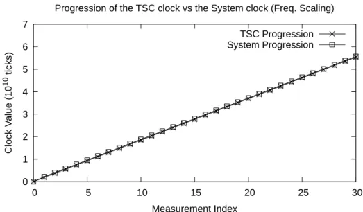
and the y-axis shows the measured value. Since the offset between the TSC and the system clock is large, we normalize the y-axis values by subtracting the first measurement (otherwise, the graph would show two horizontal lines.) We only show a subset of the sample data to make the chart readable, since we perform a lot of measures. These results show that clock drift is a linear function and a linear regression can be used to implement it. Particularly in the case with frequency scaling disabled, both lines overlap and the graph appears to only show one line. This happens because they are advancing at the same rate always, due to the CPU always working at the maximum frequency. With frequency scaling enabled, the lines do not overlap but the distance between them is constant, which still means that the clock drift is a linear function.

0 1 2 3 4 5 6 7

0 5 10 15 20 25 30

Clo

ck

Value

(10

10 tic

ks)

Measurement Index

Progression of the TSC clock vs the System clock (No Freq. Scaling) TSC Progression System Progression

(39)

3. TMTRACER- A LIGHTWEIGHTLIBRARY FORJAVAPROGRAMS 3.3. Trace Generation

0 1 2 3 4 5 6 7

0 5 10 15 20 25 30

Clo

ck

Value

(10

10 tic

ks)

Measurement Index

Progression of the TSC clock vs the System clock (Freq. Scaling) TSC Progression System Progression

Figure 3.4: Progression of the system clock vs the TSC core clock, with frequency scaling enabled. (The lines almost overlap.)

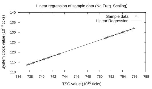
Given that clock drift is linear we can build a linear regression to model the offset of each TSC core clock against the system clock. We take sample data to capture the state of the clocks before and after the program execution. We then construct a linear regression for each core. Figures 3.5 and 3.6 show the functions built from the sample data, with frequency scaling disabled and enabled, respectively. With frequency scaling disabled, the function follows the sample data perfectly. However, when frequency scaling is enabled, each isolated sampling phase shows a linear behavior but the linear regression can’t follow it and deviates a bit on certain parts. This happens because the benchmark forces all CPU cores to work at 100% during the entire sampling execution. As such, frequency scaling does not affect the behavior of the clocks during the sample phases but it does affect their behavior during program execution.

3.3 Trace Generation

TribuSTM [Dia+12] is a fork of DeuceSTM [Kor+10] developed in FCT-UNL that pro-vides a transactional memory runtime environment for Java programs. Like DeuceSTM, it was developed with modularity in mind and allows for the implementation and usage of different STM algorithms. It uses an adaptation of JTraceView’s tracing library to gener-ate execution logs. Regular Java source code is compiled and the genergener-ated Java bytecode is instrumented by TribuSTM. This is when methods marked with the @Atomic annota-tion are transformed into transacannota-tions. Addiannota-tional meta-data is also added and memory accesses are wrapped in function calls. It can deal with multi-dimensional arrays with no limitations. It also provides an implementation of the STAMP [CM+08] benchmark.

(40)

110 115 120 125 130 135 140

736 738 740 742 744 746 748 750 752 754 756 758

S

yst

em

clo

ck

va

lue

(10

10 tic

ks)

TSC value (1010_ticks)

Linear regression of sample data (No Freq. Scaling)

Sample data Linear Regression

Figure 3.5: Linear regression of sample data, with frequency scaling disabled.

725 730 735 740 745 750 755

168 170 172 174 176 178 180 182 184 186

S

yst

em

clo

ck

va

lue

(10

10 tic

ks)

TSC value (1010_ticks)

Linear regression of sample data (Freq. Scaling)

Sample data Linear Regression

(41)

the transactions. We modified the implementation of the TL2 algorithm in TribuSTM so that each thread registers transactional events (start, commit, abort, read and write) during the execution of a TM program for a configurable time interval. The events are registered in a local buffer for each thread and each buffer holds its events sorted by execution order, since they are registered sequentially. If this buffer fills up, no subsequent events are recorded by the thread. The buffers are kept in memory during the execution and flushed to a merged binary log file when the TM program terminates. We can look at each thread’s log as a queue of events, since they are recorded sequentially for each thread, they are already in the right order. The logs are merged by looking at which event at the head of each thread’s queue has the smallest timestamp, removing it from its queue and writing it to the merged log. The merging stops when there are no events left (i.e., all events are in the merged log). This way, the order of events in a thread is preserved in the global log.

The threads may migrate between cores causing temporal inconsistencies in the trace log, due to the clock drift among the cores. Consider the trace generated with three threads depicted in Figure 3.7. Threads 1 and 2 contain no temporal inconsistencies, while Thread 3 contains one between its second (middle) and third (top) events, presumably due to a core migration. In this example, the merging of the thread logs proceeds by taking the events with timestamp 1, 2, 3, 5, 6, 7, 4, 8 and 9. Since the order of events of each thread is preserved, Thread 3’s temporal inconsistency is preserved in the merged log as well. This illustrates the merging of the logs so we do not correct the timestamps.

Time Thread 1

TS = 9

TS = 3

TS = 1

Thread 2

TS = 8

TS = 6

TS = 2

Thread 3

TS = 4

TS = 7

TS = 5

Merged Log

TS = 1 TS = 2 TS = 3 TS = 5 TS = 6 TS = 7 TS = 4 TS = 8 TS = 9

Figure 3.7: Merging the logs of three threads into a global log.

Each event has information relative to the transaction it comes from and the timestamp information recorded. The traced events have the following structure:

• Timestamp: the timestamp read from the TSC core clock;

(42)

3. TMTRACER- A LIGHTWEIGHTLIBRARY FORJAVAPROGRAMS 3.4. Verifying Log Consistency

• Event Type: the id of the type of the transactional event (start, commit, abort,

read, write);

• Thread Id: the id of the tracing thread;

• Transaction Id: the id relating to the transaction code;

• Instance Id: the id of the transaction instance;

• Address: the address that is read/written to (only for read/write);

• Value: the value written to the address (only for writes).

Although the events are relatively small in size, a large number of them are executed and recorded, specifically the memory accesses (read and writes). This leads to logs of very large size, in the order of Gigabytes for traces of 10 seconds. All of the events have the same size which allows a simple way to process the logs. The address and value fields are written with zeros on events that don’t use them.

3.4 Verifying Log Consistency

Analyzing large logs can be a problematic process, as it is not feasible to load them entirely into memory. Since the log is composed by the threads’ recorded time lines, we need only to look through each thread sequentially to analyze the events. As such, we implemented a framework that reads parts of the log into a buffer, analyzes the events in the buffer and continues to load from the log into the buffer until the end of the log. This is a viable option because every event has the same size and so the only requirement is that the buffer size be a multiple of the event size. We provide abstract methods for analyzing an event, this usually means comparing it with the previous event and storing the information on some global data structure, and performing a final operation, which we generally use as output.

As previously mentioned, trace logs may have two kinds of inconsistencies: temporal inconsistencies and operational inconsistencies. If we aim at eliminating inconsistencies from trace logs, it is important to develop a methodology for measuring or verifying the their consistency.

Each tracing thread generates a log of the recorded events, and each thread’s logs are merged to the global log file. This way, the log contains each thread’s perceived time lines. To verify the temporal consistency, we look through each of the tracing thread’s time lines to see if there are timestamps in the wrong order. In other words, we verify that for each thread, if event e1 precedes event e2, then e1’s timestamp is less than or equal thane2’s timestamp.

(43)

3. TMTRACER- A LIGHTWEIGHTLIBRARY FORJAVAPROGRAMS 3.4. Verifying Log Consistency

(44)

(45)

4

Validation

This chapter presents the experimental validation of this work. For our tests we used TribuSTM as a runtime environment and the benchmarks were executed on the Sun Fire machine from Section 3.2. We performed the experimental validation using 8, 16 and 32 (from half to the double of the number of cores) threads, with frequency scaling disabled and enabled.

Our evaluation focused on three aspects:

• The precision of our correction strategy;

• The feasibility of using the TSC as a global ordering key for events;

• The feasibility of using the TSC to order transactions.

4.1 Clock Synchronization

Depending on the machine setup and properties of programs, the generated execution traces may represent very differing program behaviors, some are CPU-intensive and per-form a lot operations, others are memory intensive and take up a lot of RAM, and others are hybrids of the former. Some of these run very well concurrently, others do not. Some need synchronization, some do not. When studying the relation of the core clocks with the system clock, it is important to evaluate a wide range of program behaviors and analyze how the clocks behave during the runtime.

(46)

4. VALIDATION 4.2. Tracing intrusion

Clock drift data is obtained before the program execution by sampling the values of the TSC core clocks and the system clock in each core. The values of each core clock are measured through the sampling execution, along side the system clock value. This allows us to establish the progression of the TSC clocks with respect to the system clock. With this data we analyze the logs and adjust the timestamps using the functions built from the sampling data.

Vacation The vacation application simulates an on-line travel reservation system. Clients

make reservations of various travel items. Clients can perform reservations, cancellations and updates. This application uses medium-sized transactions that take up a lot of time with moderate read and write sets. Vacation uses an efficient locking strategy that makes it a moderate contention benchmark.

Intruder The intruder simulates a signature intrusion detection system in a computer

network. The processing of packets is divided in three phases: capture, reassembly and detection. The capture phase uses a FIFO queue and the reassembly phase uses a self-balancing tree to implement a dictionary. Short transactions perform operations on these data structures with a small-sized read and write sets in a high contention environment.

Labyrinth The labyrinth algorithm finds a path in a three dimensional maze.

Transac-tions are very large and perform a lot of memory accesses. Since a transaction aborts when it has an overlapping path with another transaction, it is a high contention environment.

SSCA 2 The Scalable Synthetic Compact Applications 2 (SSCA 2) benchmark performs

operations on a large, directed, weighted multi-graph. It is implemented with adjacency arrays, whose nodes are added and accessed with transactions. The transactions are small, with small read and write sets, and perform on a low contention environment.

K-means The K-means algorithm partitions data from an N-dimensional space into

K related clusters, using small transactions and few memory accesses. The contention is inversely proportional to K, since the more clusters there are, the less likely it is that two transactions will work on the same one. We used K = 40 clusters, so it performs like a moderately low contention benchmark.

4.2 Tracing intrusion

(47)

4. VALIDATION 4.2. Tracing intrusion 0 2000 4000 6000 8000 10000 12000 14000

8 16 32

Tim

e

(m

s)

Threads

Intruder Execution Time (No Freq. Scaling)

Unmonitored Monitored

(a) Without frequency scaling.

2000 4000 6000 8000 10000 12000 14000

8 16 32

Tim

e

(m

s)

Threads

Intruder Execution Time (Freq. Scaling) Unmonitored Monitored

(b) With frequency scaling.

Figure 4.1: Execution time for the Intruder benchmark.

0 10000 20000 30000 40000 50000 60000 70000 80000 90000 100000

8 16 32

Tim

e

(m

s)

Threads

Vacation Execution Time (No Freq. Scaling) Unmonitored

Monitored

0 10000 20000 30000 40000 50000 60000 70000 80000 90000 100000

8 16 32

Tim

e

(m

s)

Threads

Vacation Execution Time (Freq. Scaling) Unmonitored

Monitored

Figure 4.2: Execution time for the Vacation benchmark.

In order for a tracing system to be viable, it must be lightweight and preserve the monitored program’s original behavior. In the case of transactional memory programs, the abort rate is a good indicator of their behavior. A transactional memory program executing in a high-contention environment will have a very high abort rate. If the monitoring introduces synchronization between the the several threads, the abort rate will be much lower and the information collected will be useless. In this section we evaluate the intrusion of our tracing system, by analyzing the execution time and abort rate of unmonitored and monitored executions. We use a very lightweight monitoring to count the abort rate (counting on aborts and on commits), the execution time is provided by TribuSTM.

(48)

4. VALIDATION 4.3. Correction precision

35 40 45 50 55 60 65 70 75

8 16 32

A

bort

%

Threads

Intruder Abort Rate (No Freq. Scaling)

Unmonitored Monitored

35 40 45 50 55 60 65 70 75

8 16 32

A

bort

%

Threads

Intruder Abort Rate (Freq. Scaling) Unmonitored

Monitored

Figure 4.3: Abort rate for the Intruder benchmark.

similarly to the execution times of the unmonitored execution. This is a good indication that the runtime behavior is preserved.

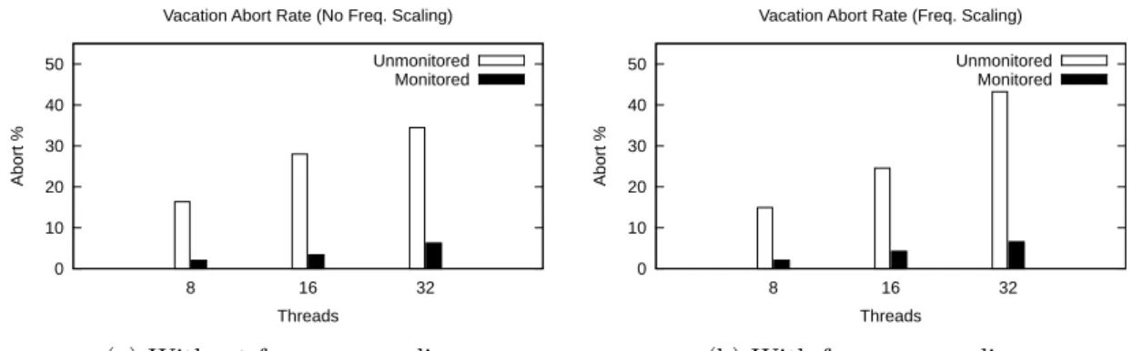
Monitoring every operation a transaction performs causes it to run slower. This is acceptable as long as the program execution retains the behavior of an unmonitored one. To more accurately measure the intrusion added by our monitoring we used the same two benchmarks (Intruder, with small transactions, and Vacation, with large transactions) and compare the abort rates of transactions of monitored executions against unmonitored ones. Figure 4.3 shows the results for the Intruder benchmark, with frequency scaling disabled and enabled respectively. The case of 8 threads suffers from the overhead caused by the monitoring. However, for the cases of 16 and 32 threads the behavior is almost exactly equal. Since Intruder benchmark performs a small number of operations per transaction, the case of 8 threads could be showing the base intrusion of our monitoring system. Figure 4.4 shows the results for the Vacation benchmark, with frequency scaling disabled and enabled respectively. Here we can see that the overhead of monitoring every event (specially reads and writes) causes a drastic change in the runtime behavior of the program. If we want to monitor every memory access performed, this becomes unavoidable in Java because we have to now also perform a JNI call for every memory access. Similar to the case of execution times, we can verify that frequency scaling does not affect the abort rate of the monitoring in a significant way.

The monitored executions run at a slower pace, however they scale in a similar fashion. The tracing preserves the behavior of programs that have small transactions almost per-fectly and impacts the behavior of programs that consistently preform large transactions.

4.3 Correction precision

(49)

4. VALIDATION 4.3. Correction precision 0 10 20 30 40 50

8 16 32

A

bort

%

Threads

Vacation Abort Rate (No Freq. Scaling) Unmonitored

Monitored

0 10 20 30 40 50

8 16 32

A

bort

%

Threads

Vacation Abort Rate (Freq. Scaling) Unmonitored

Monitored

Figure 4.4: Abort rate for the Vacation benchmark.

0 5000 10000 15000 20000 25000 30000 35000

8 16 32

Nu mber of In cons ist en cies Threads

Thread inconsistencies (Intruder - No F.S.) Total Events Before correction After correction

0 5000 10000 15000 20000 25000 30000 35000 40000 45000 50000

8 16 32

Thread inconsistencies (Intruder - F.S.) Total Events Before correction After correction

Figure 4.5: Timestamp inconsistencies for the Intruder benchmark.

events with the same timestamp to be an inconsistency as well since the TSC increases fast enough so that when an equality happens it is due to a core migration. Notice that jumps ahead in time would be another form of temporal inconsistency, however, these are harder to detect and we do not identify them. This analysis is run on each thread’s log and counts each thread’s inconsistencies and in the end the results of all threads are summed. Figure 4.5 and 4.6 show the results for a high and low contention benchmark, when frequency scaling is disabled and enabled.

(50)

4. VALIDATION 4.4. The TSC as a global ordering key 0 50000 100000 150000 200000

8 16 32

Thread inconsistencies (Vacation - No F.S.)

Total Events Before correction After correction

0 20000 40000 60000 80000 100000

8 16 32

Thread inconsistencies (Vacation - F.S.) Total Events Before correction After correction

Figure 4.6: Timestamp inconsistencies for the Vacation benchmark.

0 1000 2000 3000 4000 5000 6000 7000 8000 9000 10000

8 16 32

Nu mber of V iolat io ns Threads

Invariant violations (Intruder - No F.S.)

Before correction After correction

16000 18000 20000 22000 24000 26000 28000 30000 32000 34000

8 16 32

Nu mber of V iolat io ns Threads

Invariant violations (Intruder - F.S.) Before correction

After correction

Figure 4.7: Invariant violations for the Intruder benchmark.

4.4 The TSC as a global ordering key

One of main motivations of correcting the TSC values was so it can be used as way to order the events in the global log. For this analysis, we sorted the events in both the original log and the corrected log by their respective timestamps.

In order for the log to be well ordered, the read/write events must be in between their respective start and commit/abort operations, the commit/abort operations can only appear after their start and a transaction can only abort before it commits. As such all of this information can be captured in the regular expression:

(S (R|W)* A)* (S (R|W)* C)

Where S, R, W, A and Crepresent start, read, write, abort and commit events respec-tively. A log is correctly ordered when its order of events follow the regular expression’s order. We count the number of times this invariant is broken in the original log and in the corrected log. After the invariant has been broken, any subsequent events are ignored until a start event is reached, i.e. until we end up in a correct state again.

BSc in Computer Science

João Miguel Castanheira Martins

Lightweight Monitoring of Transactional

Memory Programs

Orientador :

João M. S. Lourenço,

Prof. Auxiliar, Universidade Nova de Lisboa

Acknowledgements

Abstract

Resumo

Contents

List of Figures

1

Introduction

1.1

Motivation

1.2

Non-intrusive Program Monitoring

1.3

Context

1.4

Log Inconsistencies

1.5

Contributions

1.6

Outline

2

Related Work

2.1

Transactional Memory

2.2

Clock Synchronization

2.3

Time Stamp Counter

2.4

Trace Generation

2.5

JTraceView

3

TMTracer - A Lightweight Library

for Java Programs

3.1

Approach

3.2

Estimating the clock drift

3.3

Trace Generation

3.4

Verifying Log Consistency

4

Validation

4.1

Clock Synchronization

4.2

Tracing intrusion

4.3

Correction precision

4.4

The TSC as a global ordering key