HBT Interferometry: Historical Perspective
Sandra S. Padula
Instituto de F´ısica Te´orica - UNESP, Rua Pamplona 145, 01405-900 S ˜ao Paulo, Brazil
Received on 15 December, 2004
I review the history of HBT interferometry, since its discovery in the mid 1950’s, up to the recent developments and results from BNL/RHIC experiments. I focus the discussion on the contributions to the subject given by members of our Brazilian group.
1
Introduction
I will discuss the fascinating method invented decades ago, which turned into a very active field of investigation up to the present. This year, we are celebrating the50th anniver-sary of the first publication of the phenomenon observed through this method. In this section, I will briefly tell the story about the phenomenon in radio-astronomy, the subse-quent observation of a similar one outside its original realm, and many a posteriori developments in the field, up to the present.
1.1
HBT
Figure 1. Aerial photo and illustration of the original HBT appara-tus. They have been extracted from Ref.[1].
HBT interferometry, also known as two-identical-particle correlation, was idealized in the 1950’s by Robert Hanbury-Brown, as a means to measuring stellar radii
through the angle subtended by nearby stars, as seen from the Earth’s surface.
Figure 2. Picture of the two telescopes used in the HBT experi-ments. The figure was extracted from Ref.[1].
two correlators, as a consequence of Bose-Einstein statis-tics. A very interesting review about these early years was written by Gerson Goldhaber[1], one of the experimentalists responsible for discovering the identical particle correlation in the opposite realm of HBT: the microcosmos of high en-ergy collisions.
1.2
GGLP
In 1959, Goldhaber, Goldhaber, Lee and Pais performed an experiment at the Bevalac/LBL, in Berkeley, CA, USA, aiming at the discovery of the ρ0 resonance[4]. In the experiment, they considered pp¯ collisions, at 1.05 GeV/c. They were searching for the resonance by means of the de-cay ρ0
→ π+π−, by measuring the unlike pair, π+π−,
mass-distribution and comparing it with the ones for like pairs, π±π±. Afterwards, they concluded that there was
not enough statistics for establishing the existence of ρ0. Nevertheless, they observed an unexpected angular corre-lation among identical pions! Later, in 1960, they success-fully reproduced the empirical angular distribution by a de-tailed multi-π phase-space calculation using symmetrized wave functions for LIKE particles. Being so, they concluded the effect was a consequence of the Bose-Einstein nature of π+π+ andπ−π−. They were not aware of the experiment Hanbury-Brown and Twiss had performed previously. Thus, they had discovered, by chance, the counterpart of the HBT effect in high energy collisions. They parameterized the ob-served correlation as:
C(Q2) = 1 +e−Q2r2= 1 +e(q20−q
2
)r2 (1)
Q2 = −q2=−(k1−k2)2=M122 −(m1+m2)2.
The Gaussian form in the above equation, and several of its variant options, would be widely used in the years to come, mainly by the experimentalists, due to the simplicity of the emission source and analytical results allowed by this pro-file. We will see which are the parameters and interpreta-tions derived from it in a while.
1.3
Simple picture
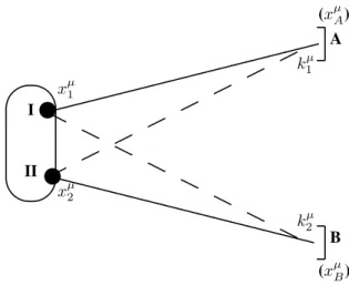
At this point, it is natural to ask the question: How to under-stand interferometry, or two-particle correlation, in a simple way? First of all, we should anticipate that it follows from considering two essential points: the adequate quantum sta-tistics and chaotically emitting sources, which was already emphasized by Bartknik and Rza¸z˙ewski[5]. Let me illus-trate it by a simple example of only two point sources, as shown in Fig. 3:
The amplitude for the process can be written as
A(k1, k2) =
1 √
2[e
−ik1.(xA−x1)eiφ1e−ik2.(xB−x2)eiφ2
± e−ik1.(xA−x2)eiφ′2e−ik2.(xB−x1)eiφ′1],(2)
where the (+) sign refers to bosons and the (−) one, to fermions. In the above equation, φi corresponds to an aleatory phase associated to each independent emission (completely chaotic sources), i.e., one phase at random in
each emission. These phases are also considered to be inde-pendent on the momentakof the emitted quanta.
②
②✘✘✘✘
✘✘✘✘
✘✘✘✘
✘✘✘✘
❳❳ ❳❳
❳❳ ❳❳
❳❳ ❳❳
❳❳ ❳❳ ❍
❍ ❍
❍ ❍
❍ ❍
❍ ✟
✟ ✟
✟ ✟
✟ ✟
✟
xµ2 xµ1
II I
(xµB) (xµA)
B A
kµ2 kµ1
✛
✚ ✘
✙
Figure 3. Simplified picture: two point sources, I and II, emit quanta considered as plane waves, which are observed in detec-tors A and B, respectively, with momentak1µandk2µ. Since the quanta are indistinguishable, there are two possible combinations for this observation, illustrated by the two continuous and the two dashed lines.
The probability for a joint observation of the two quanta with momentak1andk2is given by
P2(k1, k2) =h|A(k1, k2)|2i=
= 1
2[2±(e
i(k1−k2).(x1−x2)
he±i(φ1+φ2−φ′1−φ
′
2)i+c.c.)]
= 1±cos[(k1−k2).(x1−x2)]. (3)
The emission being chaotic, we have to consider an av-erage over random phases, i.e.,
h
e
±i(φ1+φ2−φ′1−φ′2)i
=
δ
φ1φ′1
δ
φ2φ′2+
δ
φ1φ′2δ
φ2φ′1.
(4)
The two-particle correlation function can be written asC(k1, k2) =
P2(k1, k2) P1(k1)P1(k2)
= 1±cos[(k1−k2).(x1−x2)],
(5) wherePi(ki)is the single-inclusive distribution. It is es-timated in a similar way as in the simultaneous detection discussed above, i.e.,
A(ki) =
1 √
2[e
−ik1.(xA−x1)eiφ1
±e−ik1.(xA−x2)eiφ2]
P1(ki) = h|A(ki)|2i=1
2[2±e
iki.(x1−x2)he±i(φ1−φ2)i+c.c.]
(6) In the above case, we would havehe±i(φ1−φ2)i = δ
φ1φ2.
by the same source is negligible, we would be forced to con-clude that only possible solution to this problem that would satisfy this criterium is that the average over phases is null, in the case of observation by a single detector. We see then
that Pi(ki) = 1in this case and then the result on Eq.(5)
follows.
Already from the very simple example discussed above, se can see that, in the case of two identical bosons (fermi-ons), we expect to see thatC(q = k1−k2 = 0) = 2 (0) for completely chaotic sources. On the contrary, in the case of total coherenceC(q=k1−k2) = 1for all values of the momentum difference. For large values of their relative mo-menta, however, the correlation function should tend to one, which is clearly not the case in Eq. (5). But this is merely the consequence of considering an oversimplified example of only two point sources.
1.4
Extended sources
More generally, for extended sources in space and time, if ρ(x)is the normalized space-time distribution, we have
P2(k1, k2) =
=P1(k1)P1(k2)
Z
d4x1
Z
d4x2|A(k1, k2)|2ρ(x1)ρ(x2)
=P1(k1)P1(k2)[1± |ρ˜(q)|2], (7)
where
˜
ρ(q) = Z
d4x eiqµxµρ(x) (8)
is the Fourier transform ofρ(x). Conventionally, we denote the 4-momentum difference of the pair byqµ = (kµ
1 −k µ 2), and its average byKµ= 1
2(k µ 1 +k
µ 2).
Then, the two-particle correlation function can be writ-ten as
C(k1, k2) = P2(k1, k2) P1(k1)P1(k2)
= 1±λ|ρ˜(q)|2. (9)
In Eq.(9) we added, as historically done, the parame-ter λ, later called incoherence or chaoticity parameter. This was introduced by Deutschmann et al.[6], in 1978, as a means for reducing systematic errors in the experimental fits of the correlation function. The origin of the large sys-tematic errors was the Gaussian fit. The reason was that the experimentalists tried to fit the data points with Gaussian functions whose maxima inq= 0were 2, although the data never reached that maximum value. This led to discrepan-cies and to large systematic errors. The easiest way out of this apparent inconsistency was to add a fit parameter, λ, thus reducing the systematic errors by the introduction of this extra degree of freedom.
0 0.5 1 1.5 2 2.5 3
1/R q (GeV/c) 0
0.25 0.5 0.75 1 1.25 1.5 1.75 2
C(q)
BOSONS
FERMIONS
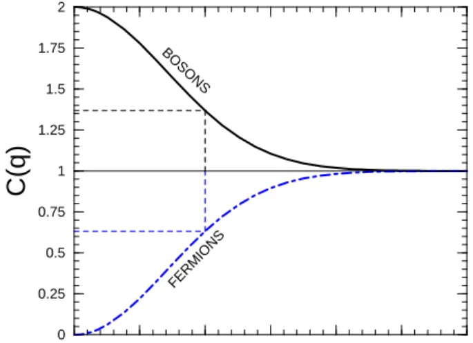
Figure 4. Simple illustration corresponding to the ideal Gaussian source. The upper curve represents to the bosonic case, while the lower curve, the fermionic one. The parameterRis the r.m.s. ra-dius of the emitting region.
To illustrate the correlation function as written in Eq.(9) with a simple analytical example, let us consider the Gaussian profile, i.e.,
ρ(x) =e−xµxµ/(2R)2 −→ ρ(q) =e−q2R2/2. (10) Consequently, in this very simple example, a typical corre-lation function is written as
C(k1, k2) = 1±λ e−q
2R2
. (11)
In equation (11), as we denoted before, the plus sign refers to the bosonic case, and the minus sign to the fermi-onic one. We easily see that, in this simple example, we would expect experimental ideal HBT data to behave as sketched in Fig. 4, where the upper part refers to bosons and the lower one, to fermions. We see that, in the two-boson (two-fermion) case, there is an enhancement (depletion) of the correlation function in the region where the relative mo-menta of the pair are small. In both cases of this simple example, the typical size of the emission region corresponds to the inverse width of theC(k1, k2)curve, plotted as a func-tion ofq=k1−k2.
value of 2 (0) for bosons (fermions) atqT = 0. Naturally, the larger the first bin size, the bigger is the deviation from the maximum (minimum) expected value for the correlation function at q = 0. This can be better seen with the help of Fig. 5, where the two upper curves represent the pure correlation function and the two lower ones, the theoretical correlation functions corrected by the Gamow factor,Υ(q), a multiplicative factor taking into account 2-body Coulomb final state interaction. This factor distorts the pattern, mainly at small values of the momentum difference of the pair, and is written as
Υ(q) = qc/q
exp(qc/q)−1
; qc= 2παm , (12) whereqis the four-momentum difference andαis the fine structure constant. The Gamow factor simply multiplies the entire expression in Eq.(9), (11), and all other forms of cor-relation function for two charged, identical particles. Fig. 5 was generated by the code CERES, whose hypothesis and formulation will be discussed later in this manuscript, in Section 2.2.
Figure 5. The plot illustrates the fact that we can have the maxi-mum of the bosonic correlation curve below unity, even when the intercept parameter is fixed to beλ= 1. This normally happens in realistic cases of finite statistics. In the plot, we see the two-pion correlation as a function ofqT, for two possible bin sizes, i.e., for
qL≤ 0.01GeV/c andqL ≤0.1GeV/c. This plot was extracted form Ref.[7]
We should emphasize, however, that the simple rela-tion between the two-particle correlarela-tion funcrela-tion and the Fourier transform of the space-time distribution, as written in Eq. (11) is not straightforward, in general. It is observed only when we can consider the phase-space as decoupled, i.e., f(x,p) = ρ(x)g(p), whereρ(x)is the source space-time distribution, andg(p)is the energy-momentum distri-bution. In general, it cannot be decoupled in this way. This is, for example, the case in relativistic heavy ion collisions, where the source expands during its life-time. The reason is that HBT is not only sensitive to the source geometry at particle emission but is also sensitive to the underlying dy-namics. This makes the analysis model-dependent and more powerful formalisms (like the one proposed by Wigner, the Covariant Current Ensemble, etc.) must be adopted. We will discuss more about this limitation later on.
1.5
Further applications
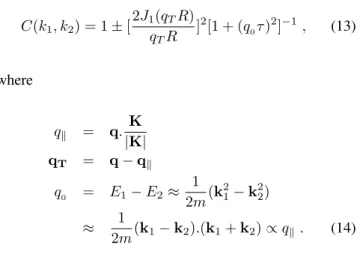
In the 1970’s, Kopylov, Podgoretski˘ı, and Grishin[8] used second-order interferometry to study several interesting problems. For example, they modelled the nucleus as a sta-tic sphere with radius R, emitting pions from its surface and got the following correlation function
C(k1, k2) = 1±[
2J1(qTR)
qTR
]2[1 + (q
0τ)
2]−1, (13)
where
qk = q.
K
|K|
qT = q−qk
q0 = E1−E2≈
1 2m(k
2 1−k22)
≈ 21m(k1−k2).(k1+k2)∝qk . (14)
The two variables in Eq.(14) are nowadays known as Kopy-lov variables. With respect to the same parametrization, Cocconi[9] re-interpreted in 1974 the quantitycτ =δ(< R)
as the thickness of the pion emission layer. They used sim-ilar forms for studying: i) the lifetime of excited nuclei through the interferometry of evaporated neutrons, ii) shape and size of multiple production region withπ±π±
correla-tions, etc. They also applied to CERN/ISR data onpp,pp¯ . Many other scientists contributed to the field during that decade. Just to mention a few names, I would quote Shuryak; Biswas; Fowler & Weiner; Giovannini & Veneziano; Grassberger; Yano & Koonin; Gyulassy, Kauff-mann & Wilson, etc. Many of these contributions were orga-nized in a collection of reprints, edited by R. M. Weiner[10], in the late 1990’s, which is a very good source of these reference papers. Among them, the papers by Gyulassy, Kauffmann & Wilson[11], as well as those by Fowler and Weiner[12], represented important steps in the field, for in-troducing more powerful formalisms for studying the cases of coherent, chaotic, and partially coherent sources. On the other hand, Grassberger[13] called the attention to the fact that resonances could play an important role in interferom-etry, since the long lived ones could distort the correlation function in the region where it was more significant, i.e., at small values of q, thus changing the chaoticity parameter
considerably. This is due to the fact that a resonance of 4-momentumk, massM, and widthΓ, would travel a distance
∼ k/(MΓ) before decaying, causing interference effects wheneverk.q≤MΓ. The first attempt to analyze the effect of resonances on interferometry in detail was made more than a decade afterwards. I will discuss it later in Sec. 2.2.
[2J1(qTR)
qTR
]2≈e−q2TR
2
T/4; 1
[1 + (q0τ)
2] ≈e −q20τ2 ,
(15) a variation of which suggests a non-relativistic parametriza-tion of the correlaparametriza-tion funcparametriza-tion, i.e.,
C(k1, k2) = 1±λ e−q
2 0τ
2/2
e−q2TR
2
T/2e−q
2
LR
2
L/2. (16) The expression in Eq. (16) has been widely employed since the beginning of high energy heavy ion collisions, be-coming the standard form to analyze two-particle interfer-ometry, particularly among the experimentalists. In Eq.(16), qL is the momentum difference along the direction of the
incident beam,qTis the component transverse to beam
di-rection, andq0 is the time component. In the late 80’s, the
most popular form changed slightly, according to the sug-gestion by Bertsch[14], becoming
C(k1, k2) = 1±λ e−q
2
SRS2e−q2OR2Oe−q2LR2L/2, (17) similarly to the previous definition. However, in Bertsch’s suggestion, there was a decomposition of the transverse component, partially incorporating the definition introduced by Kopylov and Podgoretski˘ı, i.e.,qOandqSare both
per-pendicular to beam direction but qOkKT [= 12(k1T +
k2T)], andqS⊥KT. As before,qL represents the
com-ponent of the pair momentum difference along the beam direction. Latter, Heinz et al., suggested to include a out-longitudinalcross term in Gaussian fits to the data, i.e., the correlation in this case would be written as[15]
C(k1, k2) = 1±λ e−q
2
SR
2
Se−q
2
OR
2
Oe−q
2
LR
2
Le−2q
2
OLR
2
OL . (18) Ever since, this field has been under constant develop-ment and expansion, both in the theoretical and in the ex-perimental grounds. I will briefly highlight only some of the theoretical contributions to the field, mainly focusing at the ones from the Brazilian group and some collabora-tors from abroad, since a complete discussion of the con-tribution along theses 50 years is beyond the scope of the present review. For a complete survey of the subject, as well as of the theoretical and experimental progress in the field, I would strongly encourage the reader to look into Refs. [10, 16, 17, 18, 19, 20, 21].
2
Contributions from group
mem-bers
The first contact of the group, whose contributions we are discussing here, with HBT interferometry started in the mid-to late eighties, and was the subject of my PhD Thesis[22]. In fact, it happened a few years before the group itself began performing as a group. Nevertheless, this topic consistently appeared during the group meetings along these years and, since this is a historical perspective, it is worthy to insert the subject in this context. Around the beginning of the decade of 1980, there was already an emerging subject that was attracting the attention of the high energy community: the
possible existence of a new state of matter, the Quark-Gluon Plasma (QGP), expected to be produced at high enough tem-peratures and/or densities. The QGP is a state in which quarks and gluons, the constituents of the hadrons, would be free to wander around a volume much bigger than the usual hadronic size. This state was expected to exist for a brief period of time, since only usual hadrons, with quarks and gluons confined in their interior, have been observed em-pirically. This imposed the need to look for probes of its existence. Among them, Interferometry was suggested, as a means to estimate the dimensions of the system formed in high energy collisions, thus testing if it was produced in such a new state of matter. In fact, James D. Bjorken was the person who suggested pion interferometry as the subject of my Ph.D. thesis[23].
2.1
Expansion effects in HBT
In the first paper on the subject, we started by making the hypothesis that the Quark-Gluon Plasma was already be-ing produced in pp and pp¯ collisions at the CERN/ISR. We considered[25] that the system produced in such colli-sions expanded before emitting the final particles (hadrons), according to the one-dimensional Landau Hydrodynamical Model [26]. In the initial stage, the system was formed in the QGP phase at a certain temperature,T0, started expanding and cooling down, until it reached the critical temperature, Tc, which we assumed to be of order of pion mass. It could be imagined that, once Tc was reached, the hadronization occurred instantaneously, followed by the particle emission. This simplifying hypothesis was actually adopted in the gen-eral study of the effects on the correlation function caused by the system expansion. On the other hand, the energy density of the ideal QGP fluid once Tc is reached, is much higher that the correspondent one for a hadronic system, due to the statistical degeneracy factors. More explicitly,ǫQGP(Tc) =
π 30(gg +
7 8gq)T
4
c +B, where gg = 8(color)×2(spin),
gq = 2(¯qq)×3(color)×2(spin)×Nf(f lavors)are the
gluon and quark degeneracy factors. The constantB is the vacuum pressure in the MIT Bag model. And, the hadronic correspondent for an ideal gas of pions and kaons, at Tc, is ǫπ(Tc) = 21π2[(gπ)φ(mπ/Tc) +gKφ(mK/Tc)], being gπ = 3 and gK = 4, respectively the statistical factor for pions and for kaons (The function φ(z)is a combina-tion of Bessel modified funccombina-tions of second class, Ki(z), φ(z) = z2P∞
m=0(±1)m
n
3K2[z(1+m)]
(1+m)2 +z
K1[z(1+m)]
(1+m)
o
). Nevertheless, the large ratio of the QGP to the hadronic sta-tistical degeneracy factors, together with the entropy con-servation during the phase transition, make the duration of the mixed phase very long. And mesons would be emitted during all that period. This was a more realistic hypothe-sis that was adopted when comparing our predictions with experimental data. However, for the sake of simplicity, we considered in the calculation that the emission occurred at a typical average freeze-out time,< τf >.
In our calculation, we neglected the transverse expan-sion and used the asymptotic Khalatnikov solution, i.e.
ξ ≡ ln µ
T T0
≃ −c20ln
³τ
∆ ´
α ≃ 12ln
µt+x
t−x
whereαis the system rapidity,c0 ≈1/√3is the sound ve-locityp(1−c2
0)/πl, beinglthe initial thickness of the fire-ball (solution valid wheneverξ ≫ |α|). This is essentially the Bjorken picture of hydrodynamics but with different ini-tial conditions. In the version we adopted of the hydrody-namics, the initial temperatureT0depends on the value of the fireball, with mass M, initially formed in high energy hadronic collisions. The hypothesis we used was that a large Lorentz-contracted fireball was formed around one of the in-cident particles[27], constituted of quarks and gluons, with initial radiusR≃Rproton. The fireball mass was estimated as themissing mass, i.e., by discounting the fraction of the energy available in the center of mass of thep¯(p)pcollision that was dragged by the dominant particle after the colli-sion happened. For relating this initial temperature with the fireball mass, we equated the number of produced hadrons atTc to the (conserved) entropy, which can easily be esti-mated for a QGP asS(T0) =s(T0)VQGP. The initial vol-ume of the QGP can be related to the initial energy density, ǫ0, which can be simply written as ǫ0 = M/VQGP. The initial entropy density,s(T0), can be estimated through sta-tistical relations, leaving the calculation of the initial QGP volume to be made. Since we consideredp¯(p)pcollisions, we assumed thatVQGP = 43πR30
2mp
M , whereR0andmpare, respectively, the proton radius and mass. At the end, the fi-nal proportiofi-nality coefficients were estimated with the help of the experimental data on charged multiplicity versus the missing mass. Finally, the initial temperature was related to the fireball mass by a numerical factor,T0 = 0.0989
√
M. From that, we estimatedτc, instant corresponding to the be-ginning of the phase transition,τc = ∆
³
T0
Tc
´
, and also the instant it ended,τf, as well as the typical (average) duration, < τf >(see Ref. [25] for details).
We had adopted the Kopylov variables described before, in Eq. (14) and sketched in Fig. 6, as the relevant momentum difference of the pair of pions.
Figure 6. Illustration of the Kopylov variables: we see thatq~L ≡
~
qkkK~ andq~T ≡q~⊥⊥K~. The figure also shows other notations
commonly used:~q≡∆~pandK~ ≡~p.
For studying the general behavior of the correlation function under the influence of the expansion effects, we as-sumed that each point on the surface τ = τf of the QGP, where T = Tc ≃ mπ, was an independent chaotic source with momentum spectrum given by
f(p)≃(2π1)3 uµp
µ
E exp (−
uµp µ Tc
), (20)
where uµ = (coshα,sinhα,0,0)is the 4-velocity of the fluid, and pµ = (E, p
x, py, pz)is the 4-momentum of the emitted particle. The amplitude for a particle emitted atx′
to be observed atxis written as A(x, x′) =
Z
d~ppf(p) exp [−ipµ(xµ−x′µ)]eiφ(x
′)
,
(21) where φ(x′)is a random phase. We followed the
formula-tion and notaformula-tion of Ref.[28] for writing the probability of detecting two quanta of momentap1andp2in an event, as
W(p1, p2) = ˜I(0, p1) ˜I(0, p2)+|I˜[(p1−p2),
1
2(p1+p2)]|
2,
(22) where
˜
I[(∆p), p] = Z
dx d(∆x)ei(x∆p+∆x p)
Z
dx′I(x,∆x, x′),
(23) and
hA∗[x−∆x
2 , x
′]A∗[x+∆x
2 , x
′]
i=δ(x′−x)I(x,∆x, x′). (24) The average indicated in the above equation is taken over the random phasesφ(x′)andφ(x′′). In particular, we see
that the single-inclusive distribution is written as
W(pi) =h|
Z
dx′
Z
dxeipi.xA(x, x′)dx|2i= ˜I[0, p i],
(25)
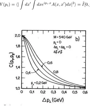
Figure 7. C(p1, p2)as a function of the momentum difference
∆pT(≡qT, in the text), for several values of the average
momen-tump⊥(≡KTin the text). A clear dependence is seen: the curves
broaden with increasing average momentum, showing a progres-sively smaller effective emission region. This plot is a reproduction of the one originally published in Ref.[25].
interesting and important results came out of that study (see Ref. [25] for details).
The first, unexpected effect, was showing a clear influ-ence of different emission times at which the pions were emitted from the source. I will write it in a simple analytical form, later in the text. This effect showed itself into the cor-relation function when plotted as a function ofqT, the Kopy-lov variable parallel to the average momentum of the pair, K= 12(k1+k2). It is illustrated in Fig. 7. Independently
of our knowledge, S. Pratt had also suggested that the time would influence the correlation function, so that large short-lived sources could result into a similar correlation function as a short long-lived one [29].
The dependence on the average momentum of the pair, KT, shown above, was a symptom of effects coming from
the underlying dynamics, and reflected the break-up of the naive picture, in which the correlation function depended exclusively on the variableqT, as in the Gaussian example
discussed above.
We also compared our results with data ofppandpp¯ col-lisions at CERN/ISR (√s= 53GeV) and could efficiently describe the trend of data. This was maybe the only success-ful description of that particular experimental result, reflect-ing the need for more powerful formalisms when describ-ing HBT interferometry at high energies. In this case, in an effort to make the estimate more realistic, we considered that the emission occurred later, at a typical instant of time < τf >, averaged over the long period that lasted the first order phase transition. We should notice that the curves in Fig. 8 are not fits, but predictions from the model, obtained without the need for introducing theλparameter (which is equivalent to fixingλ = 1). Similar treatment within the same model was also given to two-kaon interferometry data from the same experiment[25], successfully describing data.
Figure 8. In (a), the two-pion correlation function is shown in as a function of the Kopylov variableqT, averaged over the interval
qL≤0.15GeV (we adopted natural units, in which~=c= 1).
In (b), it is shown as a function of the other component,qL kK,
forqT ≤ 0.15GeV. The data points are from Ref. [24]. These
plots were originally published in Ref.[25].
Figures 7 and 8 above also show another important result from that study: the observation of strong distortions in the correlation function, definitely departing from the Gaussian shape, due to the dynamical effects related to the expansion of the system.
2.2
Non-ideal effects
More than 10 years after Grassberger pointed out the impor-tant role resonances could have in interferometry we inves-tigated it in detail, in collaboration with M. Gyulassy[30]. In particular, we analyzed the effect of resonances decay-ing into pions, followdecay-ing the predictions of resonance frac-tions from the ATTILA version of the Lund model[31]. Very briefly, it can be understood as follows: long lived reso-nances, such asω,η,η′, can mimic sources with longer
life-times, even if they freeze-out simultaneously as the direct π’s.
I call the attention to the fact that, although denoted by the same letters, the variablesqLandqT of momentum dif-ference, appearing in Fig. 9, are defined as the components parallel and perpendicular to the incident beam direction, re-spectively, as became a convention in high energy heavy ion collisions.
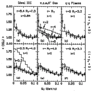
Figure 9. The two-pion correlation function is shown in three dif-ferent scenarios, as a function ofqT. The first, in parts (a) and (d)
were calculated assuming an ideal inside-outside cascade source (IOC) as in the 1-D Bjorken picture[36]. In parts (b) and (e), a non-ideal resonance gas source is considered with parameters sug-gested by the ATTILA version of the Lund model. Parts (c) and (f) correspond to the QGP model of Ref.[33]. Plots in the upper panel were calculated in the central rapidity region (2< yπ <3),
whereas the ones in the lower panel refer to1 < yπ < 2. This
figure is a reproduction of the one originally published in Ref.[30].
be seen from Fig. 9. In fact, we showed in Ref. [30] (and presented in the Quark matter ’88 Conference [34]) that the NA35 preliminary data of that time was consistent with a wider range of pion source parameters when additional non-ideal dynamical and geometrical degrees of freedom were incorporated into the analysis by extending the Covariant Current Formalism[11, 30, 35].
2.2.1 Ideal Bjorken IOC Picture
In the Covariant Current Ensemble formalism [11,30,35], the correlation function for identical bosons (since mainly bosonic HBT will be discussed in this review) can be ex-pressed as
C(k1, k2) =C(q, K) = 1 +λ |G(q, K)|
2
G(k1, k1)G(k2, k2) , (26)
whereqµ=kµ 1−k
µ
2 andKµ =12(k µ 1 +k
µ 2).
The complex amplitude,G(k1, k2), can be written as G(k1, k2) =
Z
d4xd4p eiqµxµD(x, p)j∗ 0(u
µ
fk1µ)j0(u µ fk2µ) ,
(27) whereD(x, p)is the break-up phase-space distribution[30, 37] and the currents, j0(uf.ki), contain information about the production dynamics. The one-particle spectrum is ob-tained from Eq. (27) by imposing k1 = k2, which leads to
G(ki, ki) =
Z
d4xd4p D(x, p)|j0(uµfkiµ)|2 . (28) The currentsj0(uf.ki)in Eqs. (27,28) can be associated to thermal models, and can be written in a covariant way as
j0(k)∝
p
uµk
µexp{−u µk
µ
2T }. (29)
However, to make the computation easier, we adopted a more convenient parametrization
j0(u.k) = exp{−
uµk µ
2Tps}
, (30)
where the so-called pseudo-temperatureTpsis related with the true temperatureT according to[35]
Tps(x) = 1.42T(x)−12.7MeV. (31)
This mapping between T(x)andTps(x) was later shown to be a good approximation also in the case of kaon interferometry[44].
With the covariant pseudo-thermal parametrization as in Eq. (30), the complex amplitude can be rewritten in a sim-pler form,
G(k1, k2) =heiqxafe−Kpaf/(mT)i , (32) where the bracket< ... >denote an average over the pion freeze-out phase-space coordinates.
In the case of Bjorken ideal Inside-Outside Cascade (IOC) picture, the phase-space distribution involves a fixed freeze-out proper timeτf and a perfect correlation between
ηandy. The correspondent phase-space distribution is writ-ten as
D(x, p) = 1
Ef ρ1
τf
δ(τf−τ)δ(η−y)δ(p0−Ep)g(pT) e
−x2T R2T πR2
T ,
(33) whereEp =
p
p2+m2 is the energy andg(p
T) is the transverse momentum distribution; the rapidity distribution is considered to be uniform, i.e., dNdy =ρ. In the ideal IOC picture, there is a perfect correlation in phase-space between the space-time rapidity
η=1
2ln[
t+z
t−z] (34)
and the energy-momentum rapidity, y=1
2ln[
E+pz E−pz
], (35)
i.e., they are indistinguishable.
To obtain simple analytical equations, we assume a very narrow distribution ofpT around small momenta, i.e., g(pT) = δ2(pT). The finite pion wave-packets gener-ate the finitepT distribution in our case. By substituting D(x, p) from (33) into (27) and considering the pseudo-thermal parametrization (30) for the currents, the function G(k1, k2)was found to be[35]
G(k1, k2) = 2<
dN dy >{
2
qTRT
J1(qTRT)}K0(ξ) , (36) where
ξ2 = [ 1
2Tps
(m1T +m2T)−iτ(m1T −m2T)]2+
2( 1
4T2
ps
+τ2)m
1Tm2T[cosh(∆y)−1] , (37)
and∆y=y1−y2.
The single-inclusive distribution is then written as G(ki, ki) =E
d3N dk3 i
= 2< dN
dyi > K0(
miT Tps
). (38)
To compare theoretical correlation functions with data projected onto two of the six dimensions, we computed the projected correlation function trying to mimic what is done in the experiment, i.e.,
Cproj(qT, qL) =
R
d3k
1d3k2P2(~k1, ~k2)A2(qT, qL;~k1, ~k2)
R
d3k
1d3k2P1(~k1)P1(~k2)A2(qT, qL;~k1, ~k2) ,
through which we approximate the theoretical estimate to the empirical cuts.
We should notice that, experimentally, the two-particle correlation function in high energy collisions is obtained by measuring the following ratio
Cexp(i, j) = Nexp× A(i, j)
B(i, j)
∆Cexp(i, j) = Cexp(i, j)
s
·∆A(i, j)
A(i, j) ¸2
+
·∆B(i, j)
B(i, j) ¸2
. (40)
The numeratorA(i, j)±∆A(i, j)corresponds to the com-bination of pairs of identical particles fromthe sameevent, and the denominator, B(i, j)±∆B(i, j), represents the background; Nexp is an experimental normalization. His-torically, the background for identically charged pions have been the combination of unequally charged ones. How-ever, later it was realized thatπ+π−could frequently come
from the decay of resonances, which would distort the back-ground and cause strange pattern for the correlation function built in this way. They soon realized that a better way to con-struct the background was to combine identically charged particles, but from different events. Another possibility used sometimes is a Monte Carlo simulated background, taking into account the experimental cuts and acceptance.
2.2.2 Non-ideal IOC
The non-ideal picture mentioned before referred to the un-derlying effects that would be important to incorporated into the interferometric analysis, even restricting the attention to completely chaotic sources. For instance, theπ− rapidity
distribution at 200 AGeV was clearly not uniform, as as-sumed in the asymptotic Bjorken picture, but would be bet-ter described by a Gaussian with widthYc ≈ 1.4[32]. On the other hand, a large fraction of the pions could arise from the decay of long lived resonances, such asω,K∗,η, etc,
as was suggested by Grassberger[13]. In coordinate space, the finite nuclear thickness, together with resonance effects, could lead to a large spread (∆τ) of the freeze-out proper times, and to a wide distribution of transverse decoupling radii (RT). In phase-space, there is not the perfect correla-tion between the space-time and energy-momentum rapid-ity variables present in the ideal Bjorken picture. Instead, as suggested by the ATTILA version of the Lund model, they would be better related by a Gaussian with finite width
∆η. Besides, other correlations may have to be considered if collective hydrodynamic flow occurs, for instance, between transverse coordinates (~x⊥) and transverse momentum
com-ponent (~p⊥). All these effects together were generically
called as the non-ideal picture, which is equivalent to con-sidering a more realistic picture than the one idealized by the Bjorken in his version of the 1-D hydrodynamics. The phase-space distribution representing these effects together can be obtained from Eq. (33) by replacing
ρ1 τf
δ(τf−τ)δ(η−y)→
2
∆τ2exp
à −τ2
f
∆τ2
! ×
exp ·
−(y−y
∗)2
2Y2
c
¸ 1 √
2π∆ηexp
·
−(η−y)
2
2∆η2
¸
. (41)
Besides the modification in Eq.(41), there is a major cor-rection to be added, i.e., the effect of long-lived resonances decaying into pions. This can be included in the semiclassi-cal approximation [30,34]. The pion freeze-out coordinates, xµ
a, can be related to the parent resonance production coor-dinates,xµ
r, through
xµa =xµr+uµrτ , (42) whereuµ
r is the resonance four velocity andτ is the proper time of its decay. Summing over resonances r of widths
Γr, and averaging over their decay proper times, we obtain, instead of Eq.(32) the final expression [30,34]
G(k1, k2)≈ h
X
r fπ−/r
exp(iqxr−Kur/Tr)
(1−iqur/Γr) i ,
(43)
wheref(π−/r) is the fraction of the observedπ−’s arising
from the decay of a resonance of typer, and the temper-ature Tr characterizes the decay distribution of that reso-nance. According to the Lund model, the main resonance contributing to the negative pion yield at CERN/SPS ener-gies aref(π−/ω)= 0.16,f(π−/K∗)=f[π−/(η+η′)]= 0.09,
f(π−/ρ)= 0.40,f(π−/direct)= 0.19. Although we included
direct pions and the ones coming from ρ decay indepen-dently, they are hardly distinguishable, sinceρ’s decay very fast.
All these effects combined were simulated in a Monte Carlo code, named CERES, which was also able to include simplified subroutines which mimicked the experimental cuts and acceptance[30, 34, 37].
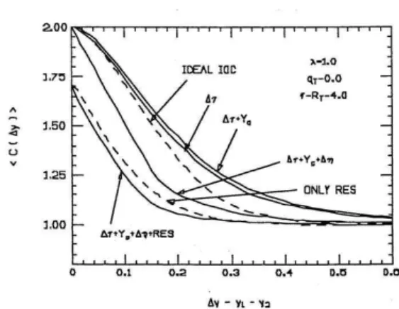
Figure 10. Numerical results for the pion correlation function ver-sus∆yare shown in the central rapidity region, when the non-ideal effects are introduced, one by one. This plot is a reproduction of the one originally published in Ref.[37].
the correlation function using the code CERES and adopt-ing the followadopt-ing values for the parameters: RT ≈ 4fm, τf ≈ 4fm/c, fixed the intercept parameterλ= 1,∆τ = 4 fm/c; Yc ≈ 1.4, ∆η ≈ 0.8, plus the above fractionsfπ/r from the Lund model, when adding resonances.
In the curves shown in Fig. 9, nevertheless, we had three sets of parameters, corresponding to the different models compared there: in the Lund resonance case, besides the fractionsfπ/r, we usedYc ≈ 1.4,∆η ≈ 0.7,RT ≈ 3fm, τf ≈3fm/c,y∗ = 2.5and fixedλ= 1; for mimicking the QGP model of Ref.[33], we used no resonance, τf = 9.0 fm/c, RT = 3.3fm, ∆η ≈ 0.76, assuming Yc → ∞and λ= 1.
The results shown previously in Fig. 9 clearly posed an-other problem to the interferometric probes of high energy heavy ion collisions: several very distinct dynamical scenar-ios could lead to approximately the same final correlation function and similar experimental HBT results.
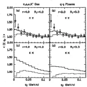
Figure 11. Comparison of two-pion, in parts (a) and (b), and two-kaon projected correlation functions, in parts (c) and (d) is considered as a function of the transverse momentum difference,
qT. The plots are calculated in the central rapidity region and with
qL≤0.1GeV. Solid (dashed) lines indicate correlations without
(with) Coulomb distortions. Parts (a) and (c) correspond to predic-tions based on the Lund model[31], and parts (b) and (d), to the plasma hydrodynamical model of Ref.[33]. The pion data is from Ref.[32]. This figure was extracted from Ref.[38].
One possibility to discriminate among very different sce-narios, suggested in Ref. [38], was to explore distinct freeze-out geometries by comparing pion and kaon interferome-try. This suggestion was motivated by the fact that an en-tirely different set of hadronic resonances decay into pions than into kaons. In the first case, according to the ATTILA version of the Lund fragmentation model, long lived res-onances such as ω, η and η′, contribute to the final pion
yield, whereas, in the second case, half of the kaons are produced by direct string decay, and the other half by the decay ofK∗. On the other hand, in the QGP model
consid-ered previously in Ref.[30] for comparison, the freeze-out geometry of all hadrons was expected to be about the same.
In the case of pions, we saw from Fig. 9 that both cases led to equally good results as compared to the experimen-tal points. In the case of kaons, then, an entirely different behavior would be expected. Indeed, we see from Fig. 11 a more significant difference between those two models, help-ing to separate long-lived scenarios from those where HBT results were generated by the effect of resonances.
Figure 12. Negative pion correlation inpp¯ and ppreactions at CERN/ISR energies are shown as a function ofQinv on the left
plot, and as function ofqT (withqL ≤0.15GeV/c) on the right
plot. Dashed, solid and dot-dashed histograms indicate the cal-culated correlation functions with, respectively, no, half and full Lund resonance abundances. The data points are from Ref.[39] on the left, and from Ref. [24], on the right hand side. Both plots were extracted from Ref.[7].
The important role of resonances stressed above led us to investigate how would be their influence for much smaller systems at higher energies. For this, we looked intopp¯ and ppdata from CERN/ISR[39]. For simplicity, in this calcu-lation, we assumed the ideal Bjorken picture to describe the freeze-out distribution. Surprisingly, the result[40] turned out to be neither compatible with the absence of resonance nor with the full resonance fractions predicted by the Lund fragmentation model mentioned before. Instead, the data seemed to be best described by the scenario with about half the resonance fractions predicted by the Lund model, as can be seen in Fig.12.
Meanwhile, we also derived a general and powerful formulation[41], based on the Wigner density formalism, which allows to treat complex system, by including an ar-bitrary phase-space distribution (i.e., the momentum dis-tribution, g(p), and the space-time one, ρ(x), could be entangled) and multi-particle correlations. This formal-ism corresponds to a semiclassical generalization of the n-particle phase-space distribution, in which it is allowed for a Gaussian spread of the coordinates around the classical trajectories, in order to incorporate minimal effects due to the uncertainty principle. Also, correction terms due to pion cascading before freeze-out were derived using this semi-classical hadronic transport model. Such terms, however, can be neglected if the mean free path of pions is small compared to the source size, or if the momentum transfers are small compared to the pion momenta. The main result of that investigation can be summarized by the following formula for the Bose-Einstein symmetrized n-pion invariant distribution
Pn(k1, ...,kn) ∝ h X
σ n
Y
j=1
exp£
i(kj−kσj).xj
¤
˜
with the smoothed delta function given by
˜
δ∆(k−k′, p−K) =
exp{[p−1
2(k+k′)]2/(2∆p2)}
(2π∆p2)−3/2
× exp[∆x
2
2 (k−k
′)2]. (45) The brackets < ... > denote an average over the 8n pion freeze-out coordinates{x1, p1, ..., xn, pn}, as obtained form the output of a specific transport model, such as a cascade[33] or the Lund hadronization model[31]. In the form written in Eq. (44) and (45), this formulation is ideally suited for Monte Carlo computation of pion interference ef-fects. The smoothed delta function results from the use of Gaussian wave packets with widths∆xand∆p, which de-pend on details of the pion production mechanism. The sum runs overn!permutationsσ = (σ1, ..., σn)of the indices; x, k, p, ... denote 4-vectors and all momenta are on-shell. This is a generalization of the Wigner type of formulation proposed in Ref.[28] and used in the pioneer work of HBT in the group, discussed in Section 2.1 and in Ref. [22, 25]. As a special limit, we found out that, for minimum Gaussian packets, i.e., ∆x∆p = 1/2, having ∆p ≃ mTps, where m is the particle mass andTps is the pseudo temperature of Eq. (31) we recovered the interferometric relations de-rived within the Covariant Current Ensemble formalism[11], which, for the sake of simplicity, was adopted as a first ap-proach to the study of non-ideal effects on Interferometry described above.
An equivalent alternative way of expressing Eq.(44) is [41]
Pn(k1, ...,kn)≈ hCN,ni
X
σ n
Y
j=1
D∆[q(j, σj), ~K(j, σj)],
(46) with
D∆(q, ~K) =
Z
d4x
Z
d3p eiqxD(x, ~p)˜δ∆(q, p−K), (47) whereD(x, ~p)can be given by, for example, Eq.(33), and CN,n ≡ N!/(N −n)!, wheren = 2in case of two-pion correlations, andN is the multiplicity of the event.
An interesting simple point explicitly demonstrated in Ref. [41], is the dependence of the effective transverse ra-dius on the average momentum of the pair, which was al-ready shown in Fig. 7, as one of the results of Ref.[25], and also suggested in [29]. This dependence onKT appears through the time dependence of the emission process. The demonstration was done by means of a simple Gaussian ex-ample, as in Eq. (16). For better understanding it, we should recall the definition of the average 4-momentum of the pair, Kµ, and their difference,qµ, i.e.,
qµ= (k1µ−k µ
2) ; Kµ=
1
2(k
µ 1 +k
µ
2). (48)
From the above relations, it immediately follows that qµKµ=q0K0−q.K≡0→q0=
q.K EK =
qT.KT+qLKL
EK ,
(49)
whereEK =√K2+m2 was written for the sake of sim-plicity.
Propagating the above result into the Gaussian correla-tion funccorrela-tion, we get
RT2ef f ≈ 2R 2
T + (∆τ)2(K2T/EK2) R2
Lef f ≈ R 2
L+ (∆τ)2(KL2/EK2). (50) The results on Eq. (50) show that the time spread of the source freeze-out generally enhances the effective size mea-sured by interferometry.
I should remark that several contributions and invited talks presented in international conferences in the period are being omitted here, due to the lack of space. I would ad-dress to the Quark Matter Conference proceedings for that, as well as the proceedings of the RANP Conference and of Hadron Physics.
2.3
Discriminating different dynamical
sce-narios
The coincidental agreement with data of two opposite sce-narios, such as the resonance gas and the QGP discussed before, in Fig. 9, stressed the necessity of finding other means to more clearly discriminate among different decou-pling geometries. Although the comparison of kaon with pion interferometry was shown to be helpful, as seen in Fig. 11, it still lacked from more quantitative information. Then, how to disentangle different models in a more precise way?
In order to answer this question, M. Gyulassy and my-self developed a method, in which a 2-Dχ2 analysis was performed, comparing two-dimensional theoretical and ex-perimental pion interferometry results[42]. For illustrating the method we performed the calculations using the code CERES mentioned above, for two very distinct scenarios. The first one considered the effects of resonances decay-ing into pions, includdecay-ing Lund resonance fractions. The other one ignored the contribution of resonances. The data points were kindly sent to us by Richard Morse, from the BNL/E802 Collaboration, and corresponded toSi+Au col-lisions at 14.6 GeV/c[43], as measured at the BNL/AGS. I will summarize the method by recalling Eq. (39) and Eq. (40). The E802 experimental acceptance functions for two particles was approximated by
A2(qT, qL;~k1, ~k2) =A1(~k1)A1(~k2)Θ(20− |φ1−φ2|)
δ(qL− |kz1−kz2|)δ(qT − |~kT1−~kT2|) . (51)
The angles are measured in degrees and the momenta in GeV/c. The single-inclusive distribution cuts were specified by
A1(~k) = Θ(14< θlab<28)
Θ(plab<2.2 GeV/c)Θ(ymin>1.5) (52).
The input temperature matching the experimentally ob-served pion spectrum wasT ≈170MeV.
the(qT, qL)plane, binned withδqT =δqL = 0.01GeV/c. Theχ2variable was computed (as suggested by W. A. Zajc) through the following relation[42]
χ2(i, j) = [A(i, j)− Nχ
−1C
th(i, j)B(i, j)]2
{[∆A(i, j)]2+ [N
χ−1Cth(i, j)∆B(i, j)]2} ,
(53) where Nχ is a normalization factor estimated as to mini-mize the average χ2, which depends on the range in the qT, qL plane under analysis. The minimization of the av-erage χ2 was performed by exploring the parameter space of the transverse radiusRT and the timeτ, and computing the< χ2 >, averaging over a 30x30 grid in the relative re-gionqT, qL < 0.3 GeV/c of relevant HBT signal. In the vicinity of the minimum we determined the parameters of the quadratic surface
hχ2(RT, τ)i=χ2min+α(RT−RT0)
2+β(τ
−τ0)2 . (54) The quantitative differences could be seen in a 3-D plot of the correlation function, projected in terms ofqT andqL, shown in Fig. 13. The main results in the case of Gamow corrected data (i.e., where the HBT signal has recovered at small values of q by multiplying by the inverse of the Gamow factor,Υ(q)−1, defined in Eq. (12)), are shown in Table 1. For a more complete discussion of the method, I would address the full article, in Ref.[42].
0.05 0.1 0.05
0.1 1
1.251.5
1.752
0.05 0.1 0.05
0.1 1
1.251.5
1.752
0.05 0.1 0.05
0.1 1
1.251.5
1.752
0.05 0.1 0.05
0.1 0 0.1 0.2 0.3 0.4
0.05 0.1 0.05
0.1 0 2 4 6 8
0.05 0.1 0.05
0.1 0 2 4 6 8
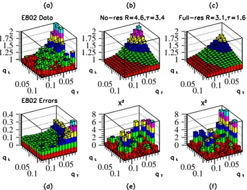
Figure 13.π−π−correlations in central Si+Au collisions is shown as a function ofqT andqL. The preliminary E802 data[43] cor-rected for acceptance and Coulomb effects are shown in part (a). Parts (b) and (c) show theoretical correlation functions filtered with the E802 acceptance. They correspond, respectively, to cases with-out and with resonance production. This figure was extracted from Ref.[42].
TABLE 1. 2D-χ2Analysis of Pion Decoupling Geometry
χ2(RT,∆τ) No Resonances LUND Resonances E802 Data Gamow Corrected
|χ2min−1|/σ 2.1 2.2 R0T 4.6±0.9 3.1±1.3
∆τ0 3.4±0.7 1.6±1.0
α 0.027 0.014
β 0.042 0.023
We see from the upper plots in Fig. 13 that the 2-D cor-relation function for the non-resonance case is clearly dif-ferent from the resonance scenario but only at very small values of the momentum differenceqT andqL. Neverthe-less, if we look into the lower panel where we plotted theχ2 distribution of the theoretical curves compared to the exper-imental points, we see that the distinction is blurred by the large fluctuations of data, mainly at the edge of the accep-tance. The most efficient measure of the goodness of the fit in this case was obtained by studying the variation of the av-erage< χ2>per degrees of freedom in the (q
T, qL) plane with respect to the unity, i.e.,| < χ2
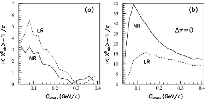
min > −1|/σ. In this way, we found out that the resolving power of the distinc-tion between different scenarios was magnified, as shown in Fig. 14.
0.0 0.1 0.2
Qmax (GeV/c)
0.0 1.0 2.0 3.0 4.0 5.0 6.0 7.0
|
〈χ
2〉
-1| (N/2)
1/2
Number of Standard Deviations from χ2=1
Lund Resonances No resonances
Figure 14. The plot shows the number of standard deviations from unity, of the average< χ2>per degree of freedom, as a function of the rangeQmaxof the analysis in the(qT, qL)plane. This plot was extracted from Ref.[42].
The method was further tested later, in a more challeng-ing situation[44], by comparchalleng-ing the interferometric results ofK+K+ of two distinct scenarios, i.e., Lund predicted resonances (onlyK∗’s and direct kaons contribute signif-icantly to this particle yield) with the non-resonance case. This was done by Cristiane G. Rold˜ao in her Master Dis-sertation, under my supervision. The data onK+K+ inter-ferometry fromSi+Aucollisions at14.6GeV/c was sent to us by Vince Cianciolo, from E859 Collaboration (an up-grade of the previous E802 experiment at BNL/AGS).
TABLE 2. 2D-χ2Analysis of Kaon Decoupling Geometry
χ2(RT,∆τ) No Resonance LUND Res.
(fKdir= 1) (fKdir=fK/K∗= 0.5)
OptimizedRT and∆τ
hχ2mini30×30 1.03 1.02 hχ2
mini10×10 1.17 1.30
RT0 2.19±0.76 1.95±0.89
∆τ0 4.4±2.0 4.4±2.6
α 0.0410 0.0299
The acceptance function for the E859 experiment was approximated[45] by
A2(qT, qL;k1, k2) =A1(k1)A1(k2)Θ(22− |φ1−φ2|)
δ(qL− |kz1−kz2|)δ(qT − |kT1−kT2|) .(55)
The angles were measured in degrees and the momenta in GeV/c. The single inclusive distribution cuts are specified by
A1(k) = Θ(14< θlab<28)Θ(plab<2.9 GeV/c)
Θ(ymin>0.75) . (56)
In the case of kaons, the input temperature matching the ex-perimentally observed kaon spectrum wasT ≈180MeV.
2 4 6 8 10 12
0 0.5 1 1.5 2
1 2 3 4 5 6 1
3.75 6.5
0 0.5 1 1.5
1 2 3 4 5 6 7 8 9 10
0 0.5 1 1.5
1 1.5 22.5 3 3.5 4 4.5 55.5 2.5
5 0 0.5 1 1.5
Figure 15. Zone in the (RT,∆τ) plane investigated, leading to
the determination of the most probable region where the minimum hχ2
i, associated to (RT,∆τ), could be located. Parts (a) and (b)
correspond to cases where the contribution ofK⋆were ignored.
Parts (c) and (d) were estimated including their contribution to the kaon yield. In parts (a) and (c) we fixed∆τ = 0, and optimized onlyRT. Figure extracted from Ref.[44].
It was expected to be harder to differentiate both sce-narios due to the lack of contribution from long-lived reso-nances. It was found that they could still be separated, with data favoring the non-resonance scenario at the 14.6Si+Au collisions (BNL/AGS). As in the two- pion interferometric analysis, the variation of the average< χ2>per degrees of freedom in the (qT, qL) plane was the significant quantity to look at, as can be seen n Fig. 16. The main fit results found in this analysis are summarized in Table 2. For more details, see Ref.[44].
0 1 2 3 4 5 6 7
0.1 0.2 0.3 0.4 0 5 10 15 20 25 30 35 40
0.1 0.2 0.3 0.4
Figure 16. The number of standard deviations from unity of the average< χ2 >per degree of freedom is shown for increasing
number of bins. In part (a), the transverse radius parameter,RT,
and the freeze-out spread,∆τ, used for generating the theoretical plots, were optimized. In (b), onlyRTwas optimized, whereas∆τ
was fixed to be zero. Figure extracted from Ref.[44].
The tests also ruled out the possibility of a zero decou-pling proper-time conjectured by that experimental results of AGS/E859 Collaboration[45]. This can be seen from part (b) of Fig. 16: by fixing∆τ to be zero the numerical de-viations of the average< χ2>per degrees of freedom are completely meaningless.
2.4
Sonoluminescence bubble
light to the problems raised above, by estimating the very small size and life-time of the single bubble sonolumines-cence phenomenon. In fact, the simple existence of a HBT type of signal from such a collapsing bubble selects the scenario of explanation between the two classes mentioned above. This is possible because the emission processes are opposite in the case of thermal models and in the Casimir based ones. In the first case, the emission is chaotic, a con-dition that is essential for observing the two-identical parti-cle HBT correlations, and an interferometric pattern would be observable. For the Casimir type of models, however, the emission is coherent and no HBT effect would be observ-able since, in that case, the correlation function acquires the trivial valueC(k1, k2) = 1for all values ofki.
Figure 17. The upper part of the figure shows correlation functions plotted as function of∆ω=ω1−ω2=c(k1−k2). Cases A to E correspond, respectively, to the first up to the fifth examples in Table 2. The lower part, shows the geometrical form factorΦ(q) plotted as a function ofX = p
−(1/2)[d2Φ(0)/dq2]q. Figures extracted from Ref.[46].
In this work we neglect all the dynamical effects dis-cussed in the previous studies, and considered that the space and time dependence would be decoupled as well. We adopted the notation used in [50], applied for our case.
C(~k1, ~k2) = 1 +
1 2
|S˜(~q, ~K)|2
˜
S(0, ~k1) ˜S(0, ~k2)
, (57)
where
˜
S(~q, ~K) = Z
d4x e−iqxρ(x)j∗(~k1)j(~k2),
~q=~k1−~k2,K~ = (~k1+~k2)/2, andj(~ki)is the amplitude for the emission of a photon with the wave-vector~kiat the source pointx. The factor 1/2 in the second term of Eq. (57) comes from the spin 1 character of the photon[50].
We suggested a set of candidate models that could try and describe the system, as summarized in Table 3.
As far as I know, no HBT experiment has been made yet with the photons emitted by the sonoluminescence bub-ble. T. Kodama and members of his group had initiated the experiment to produce single cavitating bubbles, with inten-sion to perform the interferometric test I have just described above. In any case, the simple observation of a two-photon HBT correlation would be enough to rule out one of the two classes of models that aim at explaining the phenomenon, i.e., the ones based on the Casimir effect, in which the emis-sion is coherent. It would automatically enforce the other class of thermal models, for which the emission is chaotic.
TABLE 3. Analytic expressions for some source parameterizations and the corresponding correlation functions are shown.
Sourceρ(r, t) C(~k1, ~k2)−1
A:e−r2/2R2e−t2/2τ2 e−(∆ω)2τ2e−q2R2/2
B:δ(r−R)e−t2/2τ2 e−(∆ω)2τ2[sin(qR)/(qR)]2/2
C:Θ(R−r)e−t2/2τ2 (9/2)e−(∆ω)2τ2
{(qR)}−4 {[cos(qR)−sin(qR)/(qR)]}2
D:e−r/RΘ(3τ2−t2)
sin(∆ω√3τ)/∆ω√3τ2 1 +q2R2−4
/2
E: 9|I|2/(8µ6),
Θ( ˙R t−r)e−t2/τ2Θ(t) I=
−i√π[(1 +µz+)W(z+) − (1−µz−)W(z−)]−2µ
2.5
Continuous emission
In Section 2.2.1, we discussed the Bjorken Inside-Outside Cascade (IOC)[36] picture. It considers that, after high en-ergy collisions, the system formed at the initial timeτ =τ0, thermalizes with an initial temperature T0, evolving after-wards according to the ideal 1-D hydrodynamics, essentially the same as Landau’s version discussed in Section 2.1, but with different initial conditions. During the expansion, the system gradually cools down and later decouples, when the temperature reaches a certain freeze-out value,Tf. In this model there is a simple relation between the temperature and the proper-time, i.e.,τ∝τ0
³
T0
Tf
´3 .
space-time pointxµof the system, each particle would have a certain probability of not colliding anymore. So, the distri-bution functionf(x, p)of the expanding system would have two components, one representing the portion already free and another corresponding to the part still interacting, i.e., f(x, p) =ff ree(x, p) +fint(x, p).
In the Continuous Emission (CE) model, the portion of free particles is considered to be a fraction of the to-tal distribution function, i.e.,ff ree(x, p) = Pf(x, p) =⇒
fint(x, p) = (1− P)f(x, p)or, equivalently,
ff ree(x, p) = P
1− Pfint(x, p) . (58)
The interacting part is assumed to be well represented by a thermal distribution function
fint(x, p)≈fth(x, p) = g
(2π)3
1
exp [p.u(x)/T(x)]±1 ,
(59) which poses a constraint on the applicability of the picture, since by continuously emitting particles the system would be too dilute to be considered in thermal equilibrium in its late stages of evolution. In Eq. (59),uµis the fluid velocity atxµandT is its temperature in that point.
The fraction of free particlesPat each space-time point, xµ, was computed by using the Glauber formula, i.e.,P =
exp ³−Rtout
t n(x
′)σv
reldt′
´
,wheretout=t+(−ρcosφ+
q
R2
T −ρ2sin
2φ)/(vsinθ).
The model also considered that, initially, the energy den-sity could be approximated by a constant (i.e.,ǫ= π102T4
0 for all the points withρ ≤ RT and zero forρ > RT). Then, the probabilityP may be calculated analytically, resulting inP = (τ /τout)a; a∼31.π2022 T03τ0σvrel,wherevrel ≈1. The factorPcan be interpreted as the fraction of free parti-cles with momentumpµ or, alternatively, as the probability that a particle with momentumpµescapes fromxµ without further collisions.
Their early results for the spectra can be seen in Ref.[51] and in the review by Frederique Grassi, in this volume, which is a good source of further details and discussions on the Continuous Emission model.
Later, in collaboration with F. Grassi, Y. Hama, and O. Socolowski[52], we developed the formulation for applying this new freeze-out criterium intoππinterferometry. Natu-rally, we would like to further explore if the above model would present striking differences when compared to the standard freeze-out picture (FO). One expectation would be that the space-time region from which the particles were emitted would be quite different in both scenarios. In partic-ular, as we saw in Section 2.1 and 2.2.2, a non-instantaneous emission process strongly influences the behavior of the cor-relation function. Being so, a sizable difference was ex-pected when comparing the instant freeze-out hypothesis and the continuous emission version, since in this last one, the emission process is expected to take much longer.
For treating the identical particle correlation within the continuous emission picture, instead of using the Covari-ant Current Ensemble formalism discussed in item 2.2, we adopted a different but equivalent form for expressing the amplitudes in Eq. (26) as in Ref.[51]. Then, the single-inclusive distribution, can be written as
G(ki, ki) =
Z
d4xDµ[kµiff ree] , (60)
where Dµ is the generalized divergence operator. In Ref.[51], it was shown that, in the limit of the usual freeze-out, Eq. (60) is reduced to the Cooper-Frye integral, Eddp3N3 =
R
Tfdσµp
µf(x, p), over the freeze-out hyper-surfaceT =Tf, beingdσµthe vector normal to this surface. Or equivalently, Eq. (60 ) in the instant freeze-out picture is reduced to Eq. (28), with the currents given by Eq. (29), or even by Eq. (30), which is a simplified parametric form of describing thermal currents used for obtaining analytical results in the Bjorken picture. We see more easily that it is indeed the limit if we replace the distribution function in Eq.(59) by its Boltzmann limit. We see more clearly that Eq. (28), or Eq. (38) in the Bjorken picture, are the natural lim-its of the proposed continuous emission spectrum, in case of instant freeze-out.
Analogously, the two-particle complex amplitude is written as
G(k1, k2) =
Z
d4xeiqx
{Dµ[kµ1ff ree]}
1
2 {Dµ[kµ
2ff ree]}
1 2 .
(61) We saw above that the expression for the spectrum is reduced to the one in the Covariant Current Ensemble for-malism in the limit of the instant freeze-out. Analogously, the above expression in this limit should yield to the result in Eq. (27). We see that this is indeed the case if we re-place the individual momenta kiµ in E.(61) by the average momentum of the pair, Kµ = 1
2(k µ 1 +k
µ
2). This replace-ment is even more natural, if we remember that the Kµ is the momentum appearing in the Wigner formulation of interferomtry[29, 41, 33, 19, 53]. And, it was shown in Ref. [41] that this also is reduced to the Covariant Current En-semble for minimum packets and having the packet width equated to the pseudo-thermal temperature, as discussed in Section 2.2.2. When this is assumed, also a substantial sim-plification is obtained in Eq.(61), which could then be writ-ten as
G(q, K) = Z
d4x eiqνxν
Dµ[Kµff ree] . (62)
G(q, K) =
1 (2π)3
Z 2π
0 dφ
Z +∞
−∞
dη
(
Z RT
0
ρ dρ τFMT cosh(Y −η)×ei[τF(q0cosη−qLsinhη)−ρqTcos(φ−φq)]
+
Z +∞
τ0
τ dτ ρFKTcosφ ei[τ(q0cosη−qLsinhη)−ρFqTcos(φ−φq)]
¾
× e
−MTcosh(Y−η)/Tps(x)
(1− PF)
, (63)
whereMT =
p
K2
T+M2; M2 = KµKµ− 14qµqµ; Kµ = 12(k1µ+k µ
2);Y is the rapidity corresponding toK~,φis the azimuthal angle with respect to the direction ofK~,φqis the angle between the directions of~qandK~, and
τF =
−ρcosφ+qR2
T −ρ2sin 2φ
(kT/E)[
q
sinh2η+PF−2/a−coshη]
.
ρF = −τ(kT/E) cosφ[
q
sinh2η+PF−2/a−coshη] ±
r
R2 T −τ2(
kT E )
2sin2φ[qsinh2
η+PF−2/a−coshη]2.
⌈
The spectrum is obtained from the expression (63), by replacingKµ → kµ
i,M →m, andqµ → 0. In Eq. (63), τF andρF, whose expressions are written above, are the
limiting values corresponding to the escape probabilityPF,
which we fix to bePF ≈0.5, approximate value chosen for
the sake of simplicity and for guaranteeing that the thermal assumption still holds in systems with finite size and finite lifetime. The rest of the emission forPF >0.5is assumed
to be instantaneous, as in Eq. (36) and (38).
The complexity of the expressions for the Continuous Emission (CE) case suggested that we should look into spe-cial kinematical zones for investigating the differences be-tween this scenario and the instant freeze-out picture. For details and discussions, see Ref.[52]. I summarize some of them. First, we observed that the correlation function C(qO, qL) plotted versus the outward momentum differ-ence, qO, exhibited the well-know dependence on the
av-erage momentum of the pair, KT, discussed earlier in this section, in both cases. However, it was enhanced in the CE scenario, as expected, since the emission duration is longer
in this case than in the standard freeze-out picture. We also observed a slight variation withKT of the correlation func-tion versusqSin the CE, differently from the instant
freeze-out case, were it was absent, since we were considering only the longitudinal expansion of the system and no transverse flow. This result showed the tendency of the curve versus qSto become slightly narrower for increasingKT, an oppo-site tendency as compared to the curves plotted as functions ofqO.
We also studied more realistic situations, where the cor-relation function was averaged over kinematical zones. Us-ing the azimuthal symmetry of the problem, we defined the transverse component KT along the x-axis, such that
~
K = (KT,0, KL). We then averaged over different kine-matical regions, mimicking the experimental cuts, by inte-grating over the components of~q andK~ (except over the plotting component of~q). For illustration, we considered the kinematical range of the CERN/NA35[54] experiment on S+A collisions at 200 AGeV, as
⌋
hC(qL)i= 1 +
R180
−180dKL
R600
50 dKT
R30
0 dqS
R30
0 dqoC(K, q)|G(K, q)|2
R180
−180dKL
R600
50 dKT
R30
0 dqS
R30
0 dqoC(K, q)G(k1, k1)G(k2, k2) .
⌈
With the previous equation we estimated the average theoretical correlation functions versusqL,qOandqS, com-paring the results for CE and for FO scenarios. First, we considered the case in which the initial temperature was the same in both cases (T0= 200MeV) and compared the CE
![Figure 2. Picture of the two telescopes used in the HBT experi- experi-ments. The figure was extracted from Ref.[1].](https://thumb-eu.123doks.com/thumbv2/123dok_br/18981523.457206/1.892.115.437.584.1003/figure-picture-telescopes-experi-experi-ments-figure-extracted.webp)