638 Brazilian Journal of Physics, vol. 34, no. 2B, June, 2004
Evolution from Commensurability to Size–Effects Structures in
Three–Dimensional Billiards
N. M. Sotomayor, G. M. Gusev, and J. R. Leite.
Instituto de F´ısica da Universidade de S ˜ao Paulo, CP 66318, CEP 05315-970, SP, Brazil
Received on 31 March, 2003
We calculated the classical electron dynamics of three–dimensional electrons in a billiard system in tilted mag-netic field and analyzed the evolution of trajectories in phase space by means of Poincar´e space of sections. The low field magnetoresistanceρxxwas calculated through linear response theory and found that nonlinear
resonances between the cyclotron radiusRc, the antidot lattice perioda, and the well widthW, are reflected in
the observed magnetoresistance peaks.
1
Introduction
Advances in epitaxial growth and microfabrication tech-nology have led to the experimental realization of a quasi–three–dimensional electron billiard system, in wide
AlxGa1−xAs/GaAsparabolic quantum wells (PQW), with
high mobility [1]. These systems contain a rectangular array of cylindrical voids, with sub–micron diameter, patterned across the PQW and barrier layers. Due to the combined in-fluence of the electron magneto–focusing effect and bound-ary scattering the electron motion leads to different kinds of anomalous peaks in the experimental ρxx, at low field,
performed in tilted magnetic field [1]. These measurements also demonstrated that the oscillations do not shift continu-ously toward higher values of the field as in the case of an-tidots lattices in strictly two–dimensional systems, instead they suffer a sudden transformation into structures that were attributed to galvano–magnetic size effects. However, for the proper understanding of the experimental data, and for a determination of the role of the electron trajectories, it is necessary to calculate the carrier dynamics of a thin film with a lattice of periodical voids confined, axially, by a parabolic potential.
2
Tilted field dynamics
For the present work, we use a classical approximation for the dynamics of electrons in a 3D billiard under the influence of tilted magnetic field. Indeed the full quantum-mechanical calculations of the energy spectrum and conductivities are necessary to describe the experimental results. However, we believe that classical calculations can reproduce theρxx
curves including peak positions of the commensurate reso-nances. In this work we compare only positions of the peaks of magnetoresistance with experimental traces and consider different 3D regular trajectories and its contribution to the conductivity. For this purpose classical method works quite
effectively. In order to model the electron dynamics in an ar-ray of cylindrical voids, we depart from the single–particle Hamiltonian for a three–dimensional electron,
H = 1
2m∗(~p−e ~A) 2
+UAD(x, y) +Uw(z), (1)
we chose an angle dependent potential vector given by
~
A = (1/2)B[zcosθ−ysinθ, xsinθ,−xcosθ], where e
is the electron charge, m∗
is the electron effective mass, andΘis the angle between the magnetic field vector and the surface of the PQW sample. The modulation of the electrostatic potential has no dependence of the z coordi-nate and can be simulated by the expression,UAD(x, y) =
U0{cos(2πx/a) cos (2πy/a)}β, where β is an even inte-ger which stands for the steepness of the potential,U0is the maximum amplitude, andais the antidot lattice period. For our calculations we used the soft–potential picture and take
β = 6−8.U0is assumed to be 1.6 times the Fermi energy. The confinement along thezdirection due to the potential of the well and barriers is introduced by means of the expres-sion: Uw(z) = (1/2m∗
)Ωγzγ, whereΩandγare
param-eters that may be used to fit different profiles of the confin-ing potential. We used dimensionless variables defined by:
˜
x=x/a,y˜=y/a,z˜=z/a,t˜=t/τ0,H˜ =H/EF, and ˜
U =U/EF, whereEF is the three dimensional Fermi
en-ergy. The time is scaled by: ˜τ0 = ¡
m∗
a2
/2EF¢
1/2 , where
τ0is the time that an electron delays when travel a distance equivalent to a running at the Fermi velocity. The mag-netic field is scaled by: B0 = (2/ea)(2m∗EF)1/2, where
B0 is the value of the magnetic field which corresponds to a cyclotron radius equivalent to half the lattice period (Rc =a/2). By performing these substitutions, and
N. M. Sotomayoret al. 639
µdx
dt + B B0
(zcos(θ)−ysin(θ)
¶2
+
µdy
dt − B B0
xsin(θ)
¶2
+
µdz
dt + B B0
xcos(θ)
¶2
+
UAD+Uw. (2)
The equations of motion for the system are given by:
vx= 2
µdx
dt − B B0
(zcos(θ)−ysin(θ)
(3)
vy = 2
µdy
dt − B B0
xsin(θ)
(4)
vz= 2
µdz
dt + B B0
xcos(θ)
(5)
˙
vx=1 2
B B0
µ
vxsin(θ)−vzcos(θ)
−∂UAD
∂x (6)
˙
vy=−
B B0
sin(θ)vx−
∂UAD
∂y (7)
˙
vz=
B B0
cos(θ)vx−
∂Uw
∂z (8)
A sixth–order Runge-Kutta-Verner method was em-ployed to integrate numerically these equations of motion. When θ = 90o, the Hamilton function separates and the
motion in thex−yplane and inzdirection can be treated separately. There are two additional integrals of motion, the energy of thez−motion and thexy−motion, that are con-served individually. The resulting three–dimensional tion is a combination of a two–dimensional chaotic mo-tion with the completely integrable momo-tion along z direc-tion. Furthermore, the uncoupling of the motion also leads to chaotic motion in the x−y plane for different energies
Ez, whereEF =Ex−y−Ez,EFis the Fermi energy,Ex−y is the in–plane energy andEzthe energy alongzdirection.
Thus the dynamics is mixed and, there is a coexistence of regular and chaotic trajectories. When the magnetic field is tilted0o < θ <90o, a coupling of the degrees of
free-dom appears and the system undergoes a transition to chaos. The system has three degrees of freedom and six dynami-cal variables (x, y, z, vx, vy, vz), the electron trajectories in
phase space are confined to five–dimensional surface of con-stant energy, in this space, a Poincar´e section can be defined as the intersection of the orbits with a subspace with dimen-sion 2n−2 = 4, in correspondence with the mapping in two–dimensional systems. For a 3D integrable Hamiltonian system, with a 6D phase space, the integrable surfaces are tree–dimensional and the points belonging to the fourth– dimensional mapping must lie on 2D invariant tori. If the system turns non integrable, and the Kolmogorov–Arnold– Moser (KAM) theorem [2] is still applicable, again the inte-grable surfaces are 3D and the two–dimensional tori remain on the 4D space.
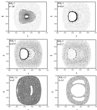
Figure 1. 2D Poincar´e projections of 4D space of sections for in-creasing tilted fields and different magnetic field values.
Figure 1, show six 2D projections (x,x˙) of the 4D space of section (x, y,x,˙ y˙) for a set of trajectories originated by a particular ensemble of initial conditions, for the same value of the normalized magnetic field B/B0 and for different values of the angle θ. This mapping was calculated for a ratio d/a = 0.22 (d is the antidot diameter), that cor-responds to an experimental sample with lattice periodic-itya = 0.5 µm. For the calculation, the initial position of thex, z coordinates, and all velocities were maintained constant. After we vary the initial position of they coor-dinate in steps of0.01aalong one of the sides of the unit cell defined by the antidot lattice perioda, The mappings correspond to the two–dimensional case of Poincar´e sur-faces of the section at y = y0 which is the intersection of the energy surface with the plane y = y0 denoted by [y(mod1) = 0]. When θ = 90o the islands correspond
to regular orbits revolving around a cylindrical void and af-ter multiple specular reflections, with the well inaf-terfaces, the electrons remain pinned by the antidot. The group of small islands, located between the innermost and outermost islands, correspond to a single quasi–periodic trajectories, and indicates that almost all phase space is filled by inte-grable KAM curves. As the tilted field increases the KAM curves are gradually deformed and destroyed and the chaotic component appears. Therefore, the distribution of chaotic points, referred as “consequents” in literature [3], fills the phase portrait at B/B0 = 1. However, for larger values of the tilted field we still observe remnants of KAM curves and stable islands for higher values ofB/B0. This feature demonstrates that nonlinear resonances are still responsible for the shifting of the commensurability peaks. Another im-portant feature is that for tilted angles less thanθ ≈ 22.5o
640 Brazilian Journal of Physics, vol. 34, no. 2B, June, 2004
the fact that the degree of coupling decrease and the sys-tem becomes again integrable in the case when the magnetic field is parallel to they direction. In PQW in tilted field, a new third length scale given by the well widthW plays an important role by allowing extra geometrical resonances, which may be responsible for the anomalous peaks in paral-lel magnetic field, as demonstrated by theρxxcalculations
showing in the next paragraph. In order to calculate the magnetoresistance we used classical linear response theory where the Ohmic conductivityσij is given, by the
expres-sion [2]:σij = m
∗e2 π~2
R∞
0 hυi(t)υj(t= 0)iΓe −t
τdt, where
~is the reduced Planck constant and< vi(t)vj(0)>Γis the velocity-velocity correlation function double averaged over phase spaceΓ, the indicesiandjstand for thexandy di-rection, respectively. The presence of impurity scattering is included through the electron mean scattering timeτ, where the probability of an electron not suffering a collision within the time interval [0,t] is given bye−t/τ
. From the numer-ical computation of the conductivity tensors σxx andσxy,
we are able to determine the longitudinalρxxand transverse
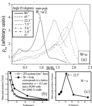
ρxyresistivities in tilted magnetic field. Figure 2(a) shows
the calculated magnetoresistance for a ratiod/a= 0.22and for a well withW =a, for different values of the angleθ. In perpendicular field we obtain two peaks corresponding to the conditionsRc=a/2andRc ≈2.0ain correspondence
which is experimentally observed. As the angleθdecreases, the peaks shift toward higher values of the normalized field. If the well is narrowW = 0.4a the behavior of the main peak tends to thesin−1
(θ)law of two–dimensional antidots in tilted magnetic field (see fig. 2(b)). However, when the well width is increasedW =awe obtain a sudden turn at the values ofθ ≈ 22.5o, that agrees with the observed in
experiments (see fig. 2(c)). These results indicate that the coexistence of geometrical resonances between the antidot period and the well width produce the anomalous behavior of the commensurability peaks in tilted field. We would like to thank FAPESP, Brazilian Funding Agency by financial support and to the LCCA-USP by computational facilities.
✂✁
Figure 2. (a) Magnetoresistance in tilted field for an antidot sample of periodicityaandW =a, (b) evolution of the main
comensu-rability peak position in tilted field forW = 0.4a, (c) the same
evolution that in (b) for a sample withW =a.
References
[1] N. M. Sotomayor, G. M. Gusev, J. R. Leite, A. A. Bykov, L. V. Litvin, N. T. Moshegov, A. I. Toropov, O. Estibals, and J. C. Portal, Physical Review B, in press (2003).
[2] R. Fleischmann, T. Geisel, and R. Ketzmerick, Phys. Rev. Lett.68, 1367 (1992).