The Spin-
1
/
2
Ising Model with Skew Magnetic Field at High Temperatures
E.V. Corrˆea Silva1, S.M. de Souza2, Onofre Rojas2, James E.F. Skea3, and M.T. Thomaz4 1Departamento de Matem´atica e Computac¸˜ao, Faculdade de Tecnologia,
Universidade do Estado do Rio de Janeiro. Estrada Resende-Riachuelo, s/no, Morada da Colina, CEP 27523-000, Resende-RJ, Brazil
2Departamento de Ciˆencias Exatas,
Universidade Federal de Lavras,
Caixa Postal 3037, CEP 37200-000, Lavras-MG, Brazil
3Departamento de F´ısica Te´orica, Instituto de F´ısica,
Universidade do Estado do Rio de Janeiro, R. S˜ao Francisco Xavier no 524, CEP- 20559-900, Rio de Janeiro-RJ, Brazil
4Instituto de F´ısica, Universidade Federal Fluminense,
Av. Gal. Milton Tavares de Souza s/no, CEP 24210-346, Niter´oi-RJ, Brazil
Received on 26 October, 2007
We calculate the thermodynamics of the one-dimensional spin-1/2 Ising model in the presence of a constant skew magnetic field. We obtain the high-temperature expansion of its Helmholtz free energy (HFE), for the ferromagnetic and antiferromagnetic cases, up to orderβ7. This expansion permits us to obtain the behaviour
of the model for|J|β<
∼1, when it cannot be described by its classical version. Among the calculated
ther-modynamical functions of the model, we have the diagonal elements of the magnetic susceptibility tensor for the transverse and logitudinal Ising models, obtained by taking the limitshz→0 andhy→0, respectively, of theβ-expansion of the HFE. They-component of the magnetization and theχyy component of the magnetic susceptibility tensor are almost the same for the antiferro- and ferromagnetic models, at least for|J|β<
∼1; and, χyyis practically independent of the direction of the external magnetic. We also show that, in this region of temperature, the thermodynamics of the Ising model with skew magnetic field and that of anX X Zmodel with longitudinal magnetic field are not similar.
Keywords: Quantized spin models; Spin chain models; Lattice theory and Statistics of Ising model; High temperature expansion
I. INTRODUCTION
The spin-1/2 Ising model with nearest-neighbor interac-tions is certainly one of the simplest one-dimensional class of models. In spite of its simplicity, it has some agreeable features. For either a purely longitudinal or purely transversal external magnetic field, it becomes exactly solvable. The ex-act thermodynamics of the longitudinal case was calculated in 1925 by Ising in his original paper[1]. In 1941 Kramers and Wannier[2] reobtained the exact thermodynamics of the Ising model in the presence of a longitudinal magnetic field by us-ing the transfer matrix approach extended to the planar model. Pfeuty[3] derived in 1970 the exact thermodynamics of the transversal Ising model, calculating its free energy; he showed the equivalence of this model to a system of noninteracting fermions, by a set of suitable transformations. One interest-ing aspect of the transversal model is its conformal invariance for a finite interval of temperature (including T =0 K), in which it has a quantum critical point (QCP)[4]. We should mention that the exact HFEs of the Ising model with longitu-dinal (hy=0) or transversal (hz=0) constant magnetic fields
are not enough to determineallthe elements of the magnetic susceptibility tensor; a more complete picture requires infor-mation on intermediary orientations of the magnetic field with respect to the easy-axis.
However the one-dimensional Ising model in the presence of a magnetic field with both longitudinal and transversal components (a skew magnetic field) is not exactly soluble: the presence of both components of the magnetic field sim-ply destroys its integrability. As an unhappy consequence, the powerful “Bethe ansatz”[5] cannot yield the exact thermody-namics of the model. The ferromagnetic version of the model, atT=0K, was studied by Fogedby[6] in the seventies. More recently, Ovchinnikov et al. studied the phase diagram, at zero temperature, of the Ising model in the presence of a skew magnetic field[7] and showed the existence of a critical line that separates the antiferromagnetic and paramagnetic states. The classical limit of this model also presents a critical line between these two states.
spin-1/2 Ising model. It is certainly interesting to have ana-lytic expansions of the thermodynamical functions of the Ising model to fit the data forarbitraryorientation of the external magnetic field. This kind of knowledge permits looking for new features of the material at finite temperatures.
The aim of the present communication is to study the ther-modynamics of both the ferromagnetic and antiferromagnetic cases of the one-dimensional spin-1/2 Ising model in the pres-ence of a skew magnetic field in the region of temperature of
|J|β<
∼1, where β=1/kT, k is the Boltzmann constant, T
is the absolute temperature in Kelvin and J is the coupling strength between first-neighbour z-components of spin (see the Hamiltonian (1)).
In section II we present the Hamiltonian of the one-dimensional spin-1/2 Ising model in the presence of a mixed magnetic field. In section III we study the thermodynamics of this model by applying the method of Ref. [9] directly to the Hamiltonian (1). The thermodynamical functions of the model depend on the sign ofJ/|J|, on the norm of the mag-netic field, on its angleθwith respect to the easy-axis, and on the temperature. One of our aims is to explicitly verify if for
|J|β<
∼1 there is any trace of the atT =0Kphase transition of
the antiferromagnetic model. In subsection III A such even-tual trace is sought by fixing the norm of the magnetic field and varying the angle θ. Its norm is such that forT =0 K andθ∈[0,θC], the system is in the antiferromagnetic state,
and forθlarger than the critical angleθC (still atT =0 K)
the system crosses the critical line of the phase diagram, pre-sented in Ref. [7]. In this subsection we consider the behav-iour of various thermodynamical quantities as functions ofθ
for a constant temperature. In subsection III B, we study the dependence of the thermodynamical functions on the temper-ature and the norm of the magnetic field and present a new du-ality between the transversal Ising model and theXY model. We also verify if the similarity of the Ising model with skew magnetic field and the X X Z model with longitudinal mag-netic field survives in the region of high temperatures. In sec-tion IV we present our conclusions. Appendix A contains the high temperature expansion of the HFE for the spin-1/2 Ising model in the presence of a mixed constant external magnetic field, up to orderβ7.
II. THE SPIN-1/2 ISING MODEL WITH SKEW
MAGNETIC FIELD
The Hamiltonian of the one-dimensional spin-1/2 Ising model in the presence of an external constant magnetic field with arbitrary orientation is
H=
N
∑
i=1
JSziSzi+1−hySyi−hzSzi
, (1)
whereSiy=σy/2 andSiz=σz/2, whereσyandσzare the Pauli
matrices. The coupling constantJcan be either positive (anti-ferromagnetic model) or negative ((anti-ferromagnetic model). The chain hasNspatial sites and it satisfies periodic spatial bound-ary conditions. Due to the symmetry of the Hamiltonian along
thez-direction (the easy-axis of the chain), the most general constant external magnetic field that we must consider can be written ash=hyjˆ+hzkˆ, where the componentshyandhzare
positive constants.
The method of Ref. [9] has been applied directly to the Hamiltonian (1) to yield the high temperature expansion of its HFE, in the thermodynamical limit (N→∞), up to order
β7. This expansion is presented in appendix (A).
From the expansion (A.1) we verify that:i) the HFE (A.1) is an even function of theyandzcomponents of the external magnetic field;ii) the HFE is sensitive to the sign ofJ(thus distinguishing between the ferromagnetic and antiferromag-netic cases) only for non-zero values ofhz. Even forhz=0
there are thermodynamical functions that can distinguish one model from the other (e.g., the first-neighbourz-component spin correlation function and thezz-component of the mag-netic susceptibility tensor).
Substitutinghy=0 orhz=0 in the expansion (A.1)
recov-ers the thermodynamics of the corresponding limiting cases of the Hamiltonian (1), given in Refs. [2] and [3], respectively.
III. THERMODYNAMICAL FUNCTIONS AT HIGH
TEMPERATURES
One can obtain the exact HFE of the one-dimensional spin-1/2 Ising model for two specific configurations of the external magnetic field; namely, the longitudinal[2] and transverse [3] ones. But that information, by itself, is not enough to infer the thermodynamic behavior for intermediary configurations of the magnetic field.
Our aim is to compare these thermodynamical functions for the ferro- and antiferromagnetic models, keeping the norm of the external magnetic field fixed, but letting its spatial orien-tation vary; i.e., by considering a magnetic field of the form
h=hsin(θ)jˆ+hcos(θ)kˆ, (2) whereh=|h|is the constant norm andθ∈[0,π/2]is the angle betweenhand thez-axis.
A. Crossing the critical line atT=0K
The spin-1/2 Hamiltonian (1) has been studied at T =0 K for the ferromagnetic[6] (J/|J| =−1) and the antiferromagnetic[7] (J/|J| =1) cases. The ground-state phase diagram [7] of the antiferromagnetic model in the pres-ence of a skew magnetic field has a critical line that separates the antiferromagnetic and paramagnetic states.
0 0 0.04 0.08 0.12
0 -0.12 -0.105 -0.09 -0.075
(a)
(b)
θ
π/2 π/2
π/4 π/4
π/8 π/8
3π/8 3π/8
J= 1
J=−1
C1
/
2
(
θ
)
ε1/
2
(
θ
)
h/|J|= 0.53 andβ|J|= 0.7
FIG. 1: (a) The specific heat per site; (b) the internal energy per site. The curves are plotted as functions ofθ, the angle between the external magnetic field vector and the easy-axis. The norm of the magnetic field, in units of|J|, is kept constant as 0.53. The angleθ
varies in the interval[0,π/2]and|J|β=0.7.
indeed crossed, forθ∈[0,π/2]. Each plot that follows com-pares the behaviour of ferromagnetic and antiferromagnetic cases under rotation of the magnetic field.
In the following figures we use the convention that the dot-ted (or dashed) and solid lines correspond to the ferromagnetic and to the antiferromagnetic model, respectively.
We begin the discussion of the thermodynamical func-tions of this model by the specific heat per site C1/2(β)≡ −β2∂2(βW1/2)
∂β2 , plotted in Fig.(1a) as a function ofθ. Atθ=0
(longitudinal magnetic field) and θ=π/2 (transverse mag-netic field) we have dCd1/2θ =0. The second derivative of this thermodynamical function is different at those two values ofθ
for the two models, but for each of them there is a single value ¯
θ, that depends weakly on the value ofβand on the model,
where d
2C
1/2
dθ2 |θ=θ¯=0. The curve of the specific heat per site is a monotonically decreasing function of θfor the antifer-romagnetic model, whereas it is a monotonically increasing function for the ferromagnetic model in the same interval ofθ
for|J|β<
∼1. For each curve, the concavity changes only once;
the value of ¯θis slightly different for the two models. The internal energy per siteε1/2(β)≡
∂(βW1/2)
∂β is plotted in
Fig. (1b). Atθ=0 andπ/2 we havedεd1/2θ =0 for both mod-els. The concavity of each curve changes at a single value of
¯
θwhich depends weakly on the value of|J|β, and is slightly different for the two models. For|J|β<
∼1, the internal energy
of the antiferromagnetic model is a monotonically decreas-ing function of θwhereas for the ferromagnetic model it is monotonically increasing.
The ferromagnetic and antiferromagnetic cases for the two thermodynamical functions in Fig. (1) coincide at θ=π/2 (transversal magnetic field) since the HFE of the Hamil-tonian (1) with a transverse magnetic field (hz=0) is
insensi-tive to the sign ofJ.
Fig. (2a) shows the first-neighbourz-component spin
cor-0 -0.03
0 0.03 0.06
0 0.648 0.654 0.66 0.666
(a)
(b)
θ
π/2
π/2
π/4
π/4
π/8
π/8
3π/8 3π/8
J= 1
J=−1
S
z iS z i+1
(
θ
)
S1/
2
(
θ
)
h/|J|= 0.53 andβ|J|= 0.7
FIG. 2: (a) The first-neighbourz-component of spin correlation func-tion. (b) The entropy for the ferromagnetic (J/|J|=−1) and antifer-romagnetic (J/|J|=1) models under the same conditions as those of Fig. (1). Both thermodynamical functions are plotted as functions of
θ∈[0,π/2].
relation functionSizSzi+1(β)≡∂W∂J1/2 forJ/|J|=1 (antifer-romagnetic case) andJ/|J|=−1 (ferromagnetic case). For both curves we have dSziSzi+1/dθ=0 atθ=0 andπ/2. As it should be, this correlation function decreases for the two models asθincreases. The concavity of the curves changes for a single value of ¯θ, that depends weakly on |J|β and on the model. Only forθ=π/2, we have thatSziSiz+1|J/|J|=1=
−SziSzi+1|J/|J|=−1, at least in the region |J|β∼<1 and for
h/|J|<
∼0.7.
The entropy per site
S
1/2(β)≡β2∂W1/2∂β for the
ferromag-netic and antiferromagferromag-netic models is plotted in Fig. (2b). The first derivative of the function
S
1/2with respect toθis zero atθ=0 andπ/2. This thermodynamical function atθ=π/2 is also the same forJ/|J|=±1, because, at this orientation of the magnetic field, the HFE is an even function ofJ. Again, the concavity of the curves, for both models, changes for a single value ¯θthat depends weakly on|J|βand on the model.
The y and z components of the magnetization per site,
M
y(1/2)(β)≡ −∂W1/2∂hy and
M
(1/2)
z (β)≡ −
∂W1/2
∂hz are presented
in Figs. (3). Fig. (3a) shows that
M
y(1/2)(θ)is almost the same for both models, at least for|J|β<∼1 andh/|J|∼<0.7. The
percentual difference between them is smaller than 3% for
θ∈[0,π/2] and the largest difference occurs aroundθ=0. This difference decreases as the value of|J|βdecreases. For
θ∼0, we have
M
y(1/2)(θ)≈aθ, and the coefficientadepends onβ. Atθ=π/2 we have dM
y(1/2)(θ)/dθ=0, forJ/|J|=±1. On the other hand,M
z(1/2) differs for the two cases (seeFig. (3b)), except atθ=π/2. Aroundθ=π/2,
M
z(1/2) is a linear function ofθ:M
z(1/2)≈b(π/2−θ). The coefficientb depends on the value ofβand on the model. We also have dM
z(1/2)(θ)/dθ=0 atθ=0.The last thermodynamical function to be discussed is the magnetic susceptibility tensor χ(i j1/2)(β)≡ −∂2W1/2
0 0 0.02 0.04 0.06 0.08
0 0 0.04 0.08 0.12
(a)
(b)
θ
π/2
π/2
π/4
π/4
π/8
π/8
3π/8 3π/8
J= 1
J=−1
M
1
/
2
z
(
θ
)
M
1
/
2
y
(
θ
)
h/|J|= 0.53 andβ|J|= 0.7
FIG. 3: TheMy1/2andMz1/2components of the magnetization per site, in (a) and (b), respectively, as functions of the angleθbetween the vector magnetic field and thez-axis. Here,|J|β=0.7 andh/|J|=
0.53.
0 0.1665
0.168 0.1695 0.171
0 0 0.4 0.8 1.2 1.6
(a)
(b)
θ
π/2
π/2
π/4
π/4
π/8
π/8
3π/8 3π/8
J= 1
J=−1
χ
1
/
2
yy
(
θ
)
∆
χyy
(%)
h/|J|= 0.53 andβ|J|= 0.7
FIG. 4: (a) The elementχ1/2yy of the magnetic susceptibility tensor versusθ, for the antiferromagnetic and ferromagnetic models, under the same conditions as the previous figures. (b) The corresponding percentual difference ofχ1/2yy , comparing the ferro- and antiferromag-netic models.
i,j∈ {y,z}. Fig. (4a) shows the componentχ(yy1/2)as a function
of θ; even at|J|β=0.7, this function for the ferromagnetic model (dashed line) is almost constant forθ∈[0,π/2]. The percentual difference of the two curves is shown in Fig. (4b); the two models have a similar value ofχ(yy1/2) for any
direc-tion of the external magnetic field. At|J|β=0.7, the largest percentual difference of this element of the magnetic suscepti-bility tensor is 3% for the two models forh/|J|<
∼0.7. Atθ=0
we haveχ(yy1/2)=0, forJ/|J|=±1. This last result cannot be
derived from the HFE of the model known in the literature[2]. The non-zero contributions to χ(yy1/2)(0)come from terms in
the expansion (A.1) of the typeJ2ph2y, where p=0,1,2 and 3. ForJ/|J|=±1, we also have dχyy(1/2)/dθ=0 atθ=0 and
π/2, and atθ=π/2 the componentχ(yy1/2)is the same for the
0 0 0.06 0.12 0.18 0.24
0 -0.004 -0.003 -0.002 -0.001 0
(a)
(b)
θ
π/2
π/2
π/4
π/4
π/8
π/8
3π/8 3π/8
J= 1
J=−1
χ
1
/
2
zz
(
θ
)
χ
1
/
2
yz
(
θ
)
h/|J|= 0.53 andβ|J|= 0.7
FIG. 5: (a)χ1/2zz versusθfor the antiferromagnetic (J/|J|=1) and ferromagnetic (J/|J|=−1) models, with |J|β=0.7 andh/|J|=
0.53. (b)χ1/2yz , under the same conditions.
ferro- and antiferromagnetic models.
Fig. (5a) shows thezz-component of the magnetic suscep-tibility tensor of the two models. The interesting point about this graph is that atθ=π/2 the value of the χ(zz1/2) is
non-zero and is different forJ/|J|=±1. We point out that, in both ferro- and antiferromagnetic cases, the expansion (A.1) shows that the rotation of the magnetic field up to theθ=π/2 configuration (i.e., a purely transverse magnetic field) yields a non-vanishingχ(zz1/2). This result cannot be derived from the
exact HFE of Ref. [3]. For the ferro- and antiferromagnetic models in the presence of a mixed magnetic field we have dχ(zz1/2)(θ)/dθ=0 atθ=0 andπ/2. The functionχ(zz1/2)(θ)for
the antiferromagnetic model is almost constant forθ∈[0,π/2] for |J|β<
∼1 and h/|J|<∼0.6, in which our β-expansion is
sound. The non-null contributions toχ(zz1/2)(θ)that give
dif-ferent contributions for the ferro- and antiferromagnetic mod-els come from the terms in theβ-expansion (A.1) of the type Jph2z, wherep=0,1,· · ·,6.
Fig. (5b) showsχ(yz1/2)(θ)for the two models; although it is
not zero, from Figs. (5) we verify that the non-diagonal ele-ments of the magnetic susceptibility tensor are much smaller than the diagonal elements, for both models. We also have
χyz(1/2)(0) =χyz(1/2)(π/2) =0 for the ferro- and
antiferromag-netic models. We are able to calculate all the elements of the tensorχ(i j1/2)(β) only if we have the Ising model (1) in the presence of a skew magnetic field.
In Figs. (1)-(5) we maintain|J|β=0.7 andh/|J|=0.53, although the features described previously in the curves of the ferromagnetic and the antiferromagnetic models, such as the monotonically increasing/decreasing behaviour of the func-tions forθ∈[0,π/2]and vanishing first derivatives atθ=0 and/orπ/2, are preserved, at least for|J|β<
∼1 andh/|J|∼<0.7,
0 0.2 0.4 0.6 0.8 1 0
0.04 0.08 0.12
0 0.2 0.4 0.6 0.8 1
0 0.05 0.1 0.15 0.2 0.25
h/|J|
C1
/
2
(
h
)
C1
/
2
(
β
)
|J|β
(a) (b)
FIG. 6: The specific heat per site atθ=0 (black curves),π/4 (red curves) andπ/2 (green curves) for the ferro- and antiferromagnetic models. In (a) the specific heat is plotted versus|J|βath/|J|=0.3; and in (b), as a function ofh/|J|at|J|β=0.7.
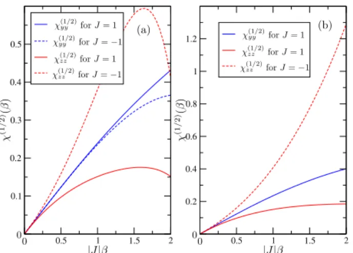
0 0.5 1 1.5 2
0 0.25 0.5 0.75 1 1.25 1.5
|J|β
χ
(1
/
2)(
β
)
χ(1zz/2)forJ=±1
χ(1yy/2)forJ= 1
χ(1yy/2)forJ=−1
FIG. 7: The diagonal components of the static magnetic susceptibil-ity tensor as functions of|J|β. The componentχ(yy1/2)corresponds to the black curve andχ(zz1/2)to the blue curve.
B. Other aspects of the thermodynamics in the region|J|β< ∼1
It is certainly interesting to check the behavior of the ther-modynamics of the model described by the Hamiltonian (1) as a function of the temperature, (or of its inverse), and its dependence on the external magnetic field.
Figs. (6a) and Fig.(6b) show the specific heat per site as a function of|J|βandh/|J|, respectively, atθ=0,π/4 andπ/2. From those figures, some aspects of the specific heat can be inferred that Fig.(1a) would not allow.
Fig.(6a) shows that the specific heat per site for|J|β<
∼0.2
and for all values ofθ∈[0,π/2]is independent of the model. This is easily understandable if we observe theβ-expansion of this thermodynamical function, derived from the HFE (A.1). From this series we obtain that the spin-1/2 Ising model in the presence of a skew magnetic field presents a tail of the Schot-tky peak[10] (CSch∝ β2), for all values ofθ. The coefficient of
theβ2-term is independent of the sign ofJ. In Fig.(6a) we take h/|J|=0.3. The black curves in this figure present the spe-cific heat of the ferro- and antiferromagnetic models atθ=0; the red curves correspond these functions atθ=π/4 and the green curve corresponds to the specific heat atθ=π/2, which is the same for both models.
Fig.(6b) shows the specific heat per site as a function of h/|J|, at |J|β=0.7, for θ=0,π/4 and π/2. At h=0, the specific heat is non-null and its value is independent of the sign ofJ. The black and red curves describe the specific heat per site atθ=0 andθ=π/4, respectively, for the ferro- and antiferromagnetic models, and the green curve corresponds to this function atθ=π/2, which is the same for both models. We point out that, in contrast to the expansion in|J|β, the ex-pansion in terms of the normh/|J|of the magnetic fieldis not exact, i.e., each coefficient in this expansion has corrections from higher orders inβ. Up to orderβ7, we obtain that the specific heat for a vanishing magnetic field is
C1/2(β)|h=0=− 17 2949120β
8J8+ 1 6144β
6J6− 1 256β
4J4+ 1 16β
2J2. (3)
The static magnetic susceptibility tensor ath=0 has only non-null diagonal elements. None of those elements can be derived from the exact HFE of the longitudinal[1] or the transversal[3] Ising models. Fig.(7) shows the yy-component of the static magnetic susceptibility tensor (χ(yy1/2)) (black curve), which is
the same for both models, and thezz-component (χ(zz1/2)) of
the ferro- (blue dashed line) and the antiferromagnetic (blue continuous line) model. In the region|J|β<
∼0.3, the elements
χ(yy1/2)andχ(zz1/2)of both models are very close. Forh=0, our
0.5 1 1.5 2 0.1
0.2 0.3 0.4 0.5
0.5 1 1.5 2
0.2 0.4 0.6 0.8 1 1.2
|J|β |J|β
χ
(1
/
2)(
β
)
χ
(1
/
2)(
β
)
χ(1/2)
zz forJ= 1
χ(1/2)
zz forJ= 1
χ(1zz/2)forJ=−1
χ(1zz/2)forJ=−1
χ(1yy/2)forJ= 1
χ(1/2)
yy forJ= 1
χ(1yy/2)forJ=−1
0 0 0
0
(a) (b)
FIG. 8: The componentsχ(yy1/2)(blue curves) andχ(zz1/2)(red curves) for the purely longitudinal and transversal magnetic field configura-tions, forh/|J|=0.3. In (a) we have the longitudinal external mag-netic field, parallel to the easy-axis (θ=0); and in (b) the transversal magnetic field, perpendicular to the easy-axis (θ=π/2).
|J|β∼2.
The componentχ(yy1/2) for the purely longitudinal (θ=0)
model is non-null. It cannot be derived from the HFE of the exact model[1]. Fig.(8a) showsχ(yy1/2) andχzz(1/2) forh/|J|=
0.3 andθ=0 (purely longitudinal external field). The blue curves representχ(yy1/2)of the ferro- and the antiferromagnetic
cases. The elementχ(yy1/2)of both models have very close
val-ues, up to|J|β∼1. There is a peak of the ferromagneticχ(zz1/2)
at|J|β=1.6342.
The componentχ(zz1/2) of the purely transversal (θ=π/2)
case is also non-null. Fig.(8b) shows the diagonal components
χ(yy1/2)andχ(zz1/2)forh/|J|=0.3 andθ=π/2. The blue curve
corresponds toχ(yy1/2), which is the same for both models; the
red curves describeχ(zz1/2)for the ferro- and antiferromagnetic
models.
For the purely longitudinal/transversal configurations of the magnetic field, the elementsχ(yy1/2) andχ(zz1/2) are of the same
order of magnitude.
The one-dimensional spin-1/2XY model,
HXY = N
∑
i=1
JxSxiSix+1+JySyiS y i+1
, (4)
(where N, the number of sites, is even) is equivalent to two spin-1/2 Ising models with transversal magnetic field (Hamil-tonian (1) withhz=0). This equivalence was demonstrated
[11] and used in the late 70’s and early 80’s to infer quantum properties from one model based on the other [12, 13]. The lattice spacing of the two Ising models is twice as large as that of theXY model.
One interesting fact also to be verified is the equivalence of the spin-1/2XYmodel, whose Hamiltonian is
HXY =
N
∑
i=1
JSxiSxi+1±2hySyiS y i+1
, (5)
to the spin-1/2 Ising model in the presence of a transversal magnetic field (Hamiltonian (1) withhz=0) at finite
temper-ature. In Ref. [14] we present the HFE of the spin-S XY Z model for an external magnetic field and with a single-ion anisotropy term, up to orderβ5. This new equivalence can be verified directly by comparing the HFE (A.1) for the spin-1/2 Ising model with transversal magnetic field (hz=0) to the
high temperature expansion presented in Ref. [14] for theXY chain (Jz=0). These HFE are calculated taking the
thermo-dynamical limit of the models; the number of sites does not need to be even, as imposed in Ref. [11]. This new equiva-lence could also be shown by the equality of the dispersion relations of the two models[5, 6].
Upon finishing the study of the thermodynamics of Hamil-tonian (1), we would like to comment on the statement in Ref. [6] where it is claimed that atT =0Kthe spin-1/2 Ising model with a skew external magnetic field (1) is “dynamically quite similar” to the special case of theXY Zmagnetic chain, that is
H′=
N
∑
i=1
Jx(SxiSxi+1−S
y iS
y i+1) +JS
z iS
z
i+1−hzSzi
. (6)
Ref. [6] suggests the existence of some relation (although un-specified therein) between the magnetic field componenthyof
the Hamiltonian (1) and the exchange parameterJxof Eq. (6),
atT=0K. In order to verify whether this would still hold for finite temperatures, we compared the thermodynamical func-tions calculated here to their results. From theβ-expansion of the HFE for theXY Z chain model [14], we verify that it depends only on even powers ofJxandJy; consequently, the
Hamiltonian (6) also describes anX X Zchain in the presence of an external magnetic field along thez-direction. In Ref. [15] we present the high temperature expansion of the spin-S X X Zmodel, with a single-ion anisotropy term and in the pres-ence of a longitudinal magnetic field (hy=0 andhz=0), up
to orderβ6.
We assume a linear relation betweenJxandhy, independent
of the value ofβ; that is,hy=aJx. In Figs. (9) we haveJ=1,
Jx=1.5 andhz=0.5. Fig. (9a) shows the percentual
differ-ence between the HFE of the Ising model (1) and that of the spin-1/2X X Zmodel (6). This curve corresponds to the mini-mum difference between the curves representing the HFEs of those models, and it is obtained by choosinga=0.7562 for
0 0.3 0.6 0.9 -0.2
-0.1 0 0.1 0.2
0 0.3 0.6 0.9
-60 -40 -20 0
(a)
(b)
β
C1/2
ε1/2
S1/2
Sz iSiz+1
M1/2
z
∆
W1
/
2
(%)
∆(%)
J= 1,Jx= 1.5,hz= 0.5 anda= 0.7562
FIG. 9: (a) The percentual difference of the HFE for the spin-1/2 models: the Ising model with a skew magnetic field and the XXZ chain in the presence of a magnetic field in the z-direction. (b) The percentual difference of the specific heat, the first-neighbourSz correlation, the entropy, the internal energy and the magnetization. Here, we letJ=1,Jx=1.5,hz=0.5 anda=0.7562.
of constants as Fig. (9a). From these curves, we verify that the entropy of the two models is similar, since the maximum percentual difference in this interval ofβ is 1.51%. On the other hand, the remaining functions are very distinct; for in-stance, the first-neighborSz correlation and the specific heat
reach percentual differences of 53.3% and 19.35%, respec-tively, atβ=0.9. From Fig. (9b) we can state that the thermo-dynamics of Hamiltonians (1) and (6) arenotsimilar, at least in the region of|J|β<
∼1.
IV. CONCLUSIONS
We derive the thermodynamics of the one-dimensional spin-1/2 Ising model (ferromagnetic and antiferromagnetic cases) in the presence of an arbitrary external constant mag-netic field, in the high temperature region (|J|β<
∼1). The
β-expansion of the HFE of the model is calculated up to or-derβ7. From expansion (A.1) we recover the known limiting cases of the model withhy=0 (longitudinal magnetic field)[2]
orhz=0 (transversal magnetic field)[3].
In the present communication, the magnetic field vector is supposed to have a constant norm and is rotated with respect to the easy-axis (z-direction) by an angleθ, which varies in the interval[0,π/2]. The phase diagram of the spin-1/2 anti-ferromagnetic Ising model with skew magnetic field exhibits a critical line, in the space of magnetic field components(hy,hz)
at zero temperature[7]. In the first part of the paper the norm of the magnetic field has been chosen to be h/|J|=0.53, such that there exists a critical angle θc for which the
zero-temperature critical line of the phase diagram is crossed, as
θvaries. The following thermodynamical functions per site are plotted as functions ofθ, for the antiferromagnetic and the ferromagnetic models at|J|β=0.7: the specific heat; the
in-ternal energy; the first-neighbourSz correlation function; the
entropy; the yandz components of the magnetization; and the elements of the magnetic susceptibility tensor. All these are smooth functions ofθin the interval [0,π/2]. Although the curves are plotted for |J|β=0.7 and h/|J|=0.53, the features presented and discussed in the text are preserved, at least, up to|J|β∼1 andh/|J| ∼0.7. In general, the curves are monotonically increasing or decreasing functions ofθ.
The y-component of the magnetization and the magnetic susceptibility component χ(yy1/2) of antiferro- and
ferromag-netic models are very close. The componentχ(zz1/2)for the
fer-romagnetic case is almost independent of theθangle. Those results are valid, at least, for|J|β<
∼1 andh/|J|<∼0.7.
Our results for the elementsχ(yy1/2) andχ(zz1/2) of the
mag-netic susceptibility tensor for the limiting caseshy=0 and
hz=0, respectively, could not be derived from the known HFE
in the literature[2, 3]. These elements are non-zero.
We verify that the spin-1/2 Ising model in a skew mag-netic field presents a tail of the Schottky peak[10] that isθ -dependent, but otherwise independent of other features of the model. We also plot the specific heat per site versus the norm of the magnetic field. This function does not vanish ath=0, and gets corrections from terms of higher orders inβ from high temperature expansion of the HFE of the model.
By explicit calculation, we verify the equivalence of the spin-1/2 Ising model in the presence of a transversal magnetic field and theXYchain, a different duality of the one known in the literature[3, 11, 13].
Finally, we verified that the thermodynamics of the spin-1/2 Ising model with a skew magnetic field is not similar to the thermodynamics of the spin-1/2 X X Z chain, at least in this region of temperature, contrary to what is claimed by Fogedby[6] to hold forT=0K.
S.M. de S. and O.R. thank FAPEMIG and CNPq for partial financial support. E.V. Corrˆea Silva (Fellowship CNPq, Brasil, Proc.No.305800/2004-3) thanks CNPq for partial financial support (Edital Universal CNPq/2006 -Proc.No.476852/2006-4). M.T. Thomaz (Fellowship CNPq, Brasil, Proc.No.: 30.0549/83-FA) thanks CNPq for partial fi-nancial support (Grants 1D). J.E.F. Skea thanks FAPERJ for financial support via a Prociˆencia research grant during part of this work.
APPENDIX A: THEβ-EXPANSION OF THE HFE FOR THE
SPIN-1/2 ISING MODEL WITH SKEW MAGNETIC FIELD
Hamiltonian (1) describes the interaction between first neighbours along the chain, subject to a periodic spatial con-dition. These two features allow us to apply the method of Ref. [9] directly to this Hamiltonian to calculate the β -expansion of its HFE.
W
1/2(β;hy,hz) = (17 645120hz
8− 107 35840J
2h
y2hz4+
17 161280hz
6h
y2−
1 1792J
2h
z2hy4
+ 17
645120hy
8+ 17 161280hz
2h
y6+
17 107520hz
4h
y4+
17 2580480J
6h
y2
+ 121
73728J 4h
z4+
17 165150720J
8+ 61 1290240J
4h
y2hz2−
107 46080J
2h
z6
+ 17
161280J 2h
y6+
17 286720J
4h
y4−
1 368640J
6h
z2)β7+ (
17 11520J hz
6
+ 17
11520J hz 2h
y4+
17 5760J hz
4h
y2−
1 1920J
3h
z2hy2−
5 1152J
3h
z4
+ 1
30720J 5h
z2)β6+ (
13 3840J
2h
z2hy2−
1 2880hy
6− 1 184320J
6− 1 2880hz
6
− 1
960hz 4h
y2−
1 960hz
2h
y4−
1 5120J
4h
y2−
1 3072J
4h
z2+
13 1536J
2h
z4
− 1
1280J 2h
y4)β5+ (
1 384J
3h
z2−
1 96J hz
2h
y2−
1 96J hz
4)β4
+ (−1
64J 2h
z2+
1 3072J
4+ 1 96hz
2h
y2+
1 192hy
4+ 1 192hz
4
+ 1
192J 2h
y2)β3+
β2J h
z2
16 + (− hz2
8 −
J2 32−
hy2
8 )β− ln(2)
β . (A.1)
The function
W
1/2(β;hy,hz)is sensitive to the sign of Jonly if hz =0. The expansion (A.1) is equally valid for
positive (antiferromagnetic case) and negative (ferromagnetic case) values ofJ.
Certainly, the proper parameter in which one could rewrite (A.1) is|J|β; therefore, the components of the external mag-netic field are measured in units of|J|.
[1] E. Ising, Z. Phys.31, 253 (1925).
[2] H.A. Kramers and G.H. Wannier, Phys. Rev.60, 252 (1941). [3] P. Pfeuty, Annals of Phys.57, 79 (1970).
[4] A. Kopp and S. Chakravarty, Nature1, 53, October (2005). [5] M. Takahashi, “Thermodynamic of One-Dimensional Solvable
Models”, (Cambridge University Press, Cambridge, 1999). [6] H.C. Fogedby, J. Phys. C11, 2801 (1978).
[7] A.A. Ovchinnikov, D.V. Dmitriev, V. Ya. Krivnov, and V.O. Cheranovskii, Phys. Rev. B68, 214406 (2003).
[8] R. Cl´erac, H. Miyasaka, M. Yamashita, and C. Coulon, J. Am. Chem. Soc124, 12837 (2002).
[9] O. Rojas, S. M. de Souza, and M. T. Thomaz, J. Math. Phys.
43, 1390 (2002).
[10] S.J. Collocott, R. Driver, L. Dale, and S.X. Dou, Phys. Rev. B
37, 7917 (1988).
[11] R. Jullien and J.N. Fields, Phys. Lett. A69, 214 (1978). [12] R. Jullien and P. Pfeuty, Phys. Rev. B19, 4648 (1979). [13] I. Peschel and K.D. Schotte, Z. Phys.- Condensed Matter B54,
305 (1984).
[14] O. Rojas, S. M. de Souza, E. V. Corrˆea Silva, and M. T. Thomaz, Phys. Rev. B72, 172414 (2005).