Braz. J. Phys. vol.35 número2A

(1)

Classical Trajectories and Quantum Field Theory

Giuseppe Vitiello

Dipartimento di Fisica “E.R.Caianiello”, Universit `a di Salerno, 84100 Salerno, Italy INFN, Gruppo Collegato di Salerno and INFM, Sezione di Salerno

Received on 11 December, 2004

The density matrix and the Wigner function formalism requires the doubling of the degrees of freedom in quantum mechanics (QM) and quantum field theory (QFT). The doubled degrees of freedom play the role of the thermal bath or environment degrees of freedom and are entangled with the system degrees of freedom. They also account for quantum noise in the fluctuating random forces in the system–environment coupling. The algebraic structure of QFT turns out to be the one of the deformed Hopf algebra. In such a frame, the trajectories in the space of the unitarily inequivalent representations of the canonical commutation relations turn out to be classical trajectories and, under convenient conditions, they may exhibit properties typical of classical chaotic trajectories in nonlinear dynamics. The quantum Brownian motion and the two-slit experiment in QM are discussed in connection with the doubling of the degrees of freedom.

I. INTRODUCTION

In this paper I consider the problem of the interplay be-tween ‘classical and quantum’ from the point of view of the intrinsic mathematical structure of Quantum Field Theory (QFT).

The emergence of classicality from Quantum Mechanics (QM) as a result of decoherence has been and is currently an-alyzed in detail in the literature. One further scenario, since long well known, is the one of the emergence of macroscopic ordered patterns out of a quantum dynamics; this is the case of the generation of classically behaving structures out of QFT (not QM!) with spontaneous breakdown of symmetry. Crys-tals, ferromagnets, superconductors, superfluids are examples of such classically behaving macroscopic quantum systems. These are quantum systems not in the trivial sense that they, as all other kind of matter, are made of quantum components, but in the sense that their macroscopic behavior, characterized by the classical (c-number) observable called order parameter, cannot be explained without recourse to the underlying quan-tum field dynamics. On the other hand, the opposite route, from classical to quantum, namely the problem of ‘quantiza-tion’ of a classical theory, is a central problem in many fields of research; paradigmatic examples are the ones of gravitation theories and of non-hamiltonian systems, such as dissipative systems. More recently, an alternative, novel perspective has been proposed [1] (see also [2–4]) for the route from classical to quantum, the one of the ‘emergence’ of the quantum-like behavior from a classical frame; namely, the possibility has been considered that classical deterministic systems with dis-sipation (information loss) may exhibit quantum behavior.

My task in this paper is to present and to discuss some re-sults related with aspects of the classical/quantum interplay in connection with the existence in QFT of infinitely many uni-tarily inequivalent representations (uir) of the canonical com-mutation (or anti-comcom-mutation) relations (ccr).

In QM the well known von Neumann theorem states that for systems with a finite number of degrees of freedom all the representations of the ccr are unitarily equivalent. Such a theorem does not hold in QFT where the systems have infinite number of degrees of freedom. Infinitely many uir of the ccr are thus allowed to exist [5–7] and therefore, in this respect,

QFT is drastically different from QM, and one is not allowed to make confusion among the two. The existence of uir is a characterizing feature of QFT and a full series of physically relevant consequences follows.

In the first part of the paper, by considering some aspects of the quantum Brownian motion and of the two-slit experiment, I discuss the role of the doubling of the degrees of freedom and show how quantum/classical features depend on it (Sec-tion II). This part, although physically interesting in itself for the nature of the considered problems, is useful for the subse-quent discussion of the deformed Hopf algebra structure[8, 9] of QFT in Section III. This is indeed analyzed in the sec-ond part of the paper and leads to recognize that a symplectic structure with classical dynamics is embedded in the space of the uir of ccr in QFT [10]. In this way, a further aspect of the classical/quantum interplay emerges as an intrinsic feature of QFT. The entanglement between the system degrees of free-dom and the doubled ones is commented upon in Section IV. In Section V trajectories in the space of the uir are shown to be classical trajectories, which, under convenient conditions, may satisfy the criteria for chaoticity prescribed by nonlinear dynamics. Section VI is devoted to conclusions.

II. THE DOUBLING OF THE DEGREES OF FREEDOM

In this Section the main observation is that in QM and in QFT a basic role is played by the doubling of the degrees of freedom of the system under study. It is well known, for example, that in thermal field theory the doubled degrees of freedom describe the heat bath [7, 11–15]; or, near a black hole, such a doubling describes the modes on the two sides of the horizon [16–18].

On a much simpler ground, the familiar operation of

adding, e.g., the angular momentumJα, α=1,2,3, of two

identical particles, is given by∆Jα=Jα_⊗1+1_⊗Jα_≡J₁α+

J₂α. Such an addition is a homomorphism which indeed

dupli-cates the algebra,∆:

A

→

A

⊗

A

, i.e.∆

O

=

O

⊗1+1_⊗

O

≡

O1

+

O2

, with

O

∈

A

. I will come back to this point in the

following and the addition operation∆will be identified with

(2)

352 Giuseppe Vitiello

It is much instructive to illustrate the formal and the phys-ical relevance of the doubling of the degrees of freedom by considering some typical problems in QM, such as the two-slit diffraction experiment and the Brownian motion of a quantum particle.

On a formal basis, one can understand the doubling of the degrees of freedom [19–21] by considering the standard ex-pression for the Wigner function [22],

W(p,x,t) =

1 2π~

Z ψ∗

µ x₋1

2y,t

¶ ψ

µ x+1

2y,t

¶

e(−ipy~)_dy. ₍₁₎

The associated density matrix function is

W(x,y,t) = (x+|ρ(t)|x−) =ψ∗(x−,t)ψ(x+,t), (2)

wherex_±=x_±1₂y. The density matrix and the Wigner

func-tion formalism thusrequiresthe introduction of a “doubled”

set of coordinates,(x_±,p_±)(or(x,px)and(y,py)).

It is possible to show [20] that the role of the “doubled”y

coordinate is absolutely crucial in the quantum regime, since there it accounts for the quantum noise in the fluctuating ran-dom force in the system-environment coupling: in the limit of

y_→0 (i.e. forx+=x−) quantum effects are lost and the

clas-sical limit is obtained. For example, this can be seen by

con-sidering the question of how a classical situation withx+=x−

arises in the formalism by Schwinger[23] and by Feynman and Vernon [24] for the quantum Brownian motion [21].

In the treatment of quantum Brownian motion one may start by describing a classical object as having a coordinate

which depends on time x(t). The density matrix formalism

then suggests that a quantum object may be described as

split-ting the single coordinatex(t)into two coordinatesx+(t)

(go-ing forward in time) andx₋(t)(going backward in time) [23].

The classical limit is obtained when both motions coincide

x(t) =x+(t) =x−(t). To see why this is the case, one may

employ the Schwinger quantum operator action principle, or recall the mean value of a quantum operator

¯

A(t) = (ψ(t)|A_|ψ(t)) = Z Z

ψ∗(x₋,t) (x₋_|A_|x+)ψ(x+,t)dx+dx−=

Z Z

(x+|ρ(t)|x−)(x−|A|x+)dx+dx−. (3)

Thus one requires the density matrix (2) to follow two copies of the Schr¨odinger equation, i.e. the forward in time motion and and the backward in time motion, respectively controlled

by the two Hamiltonian operatorsH_±:

i~∂ψ(x±,t)

∂t =H±ψ(x±,t), (4)

which gives

i~∂(x+|ρ(t)|x−)

∂t =

H

(x+|ρ(t)|x−), (5)

where

H

=H+−H−. (6)

Working with two copies of the Hamiltonian (i.e. H_±)

oper-ating on the outer product of two Hilbert spaces has been an implicit requirement in quantum mechanics since the very be-ginning of the theory. For example, from Eqs.(5), (6) one finds

immediately that the eigenvalues of the dynamic operator

H

are directly the Bohr transition frequencies~_ω_nm₌En−Em

which was the first clue to the explanation of spectroscopic structure.

The notion that a quantum particle has two coordinates

x_±(t)moving at the same time is therefore central. It is the

difference between the two motions

y=x+−x− (7)

that induces quantum interference. In the following we will show this by explicit calculation of diffraction patterns in the case of the two-slit experiment.

The second step in the description of the Brownian motion of a quantum particle requires to consider the modification of damped evolution operator in Eqs.(5), (6) which becomes, for

a Brownian particle of massM moving in a potential U(x)

with a damping resistance R, [20, 21]

H

Brownian=

H

− ikBT R

~ (x+−x−)

2_,

(8)

H

= 1

2M

µ p₊₋R

2x−

¶2

− 1

2M

µ p₋+R

2x+

¶2

+U(x+)−U(x−) (9)

i~∂(x+|ρ(t)|x−)

∂t =

H

Brownian(x+|ρ(t)|x−) =

H

(x+|ρ(t)|x−) − (x+|N[ρ]|x−), (10)

whereN[ρ]≈(ikBT R/~)[x,[x,ρ]]describes the effects of the

reservoir random thermal noise and the “Hamiltonian”

H

the

motion in the(x+,x−)plane [20, 21].

In Eq. (9)p_±=−i~ ∂

∂x_±. In general the density operator in

the above expression describes a mixed statistical state. It can be also shown [21] that the thermal bath contribution to the right hand side of Eq.(8), proportional to fluid temperature T, is equivalent to a white noise fluctuation source coupling the forward and backward motions in Eq.(7) according to

<y(t)y(t′)>noise= ~ 2

2RkBT

δ(t₋t′), (11) so that thermal fluctuations are always occurring in the dif-ference (7) between forward in time and backward in time coordinates.

The continual occurring of the forward and backward in time motions can also be seen by constructing the forward and backward in time velocities

v_±=∂

H

Brownian ∂p_± =±

1

M µ

p_±_∓R

2x∓

¶

(3)

Brazilian Journal of Physics, vol. 35. no. 2A, June, 2005 353

■

❾

ó❡❈ ❜ ❝❞✖ó❡❊ ô ❝❈

❱ ô ❾ ❊ ✜ ❿✪➏❇➐♥➒❉➓❙➈ ❳➔

➈✂ó❛❈❨❜✁❝❞✖ó❡❊ ô ❝❈

❱

ô ✜

❿ ó❡❈ ❜ ❝❞✖ó❡❊ô ❝❲❈

❱

ô ◆ ó❡❈ ❜ ❝✂ ✠❞ ✌❲❝❘❈

❱

ô ✣ ó✜☛✒❖ ô

é❪ß✏✷✹á▲✷✄✂ ✠❞ ✌✆☎ ó ❽❲➣

➏↕↔✁➙✆✝❍■

ô

✠❈✙✣✒✠❈❇✣❉❞ ✌☞✌✤ã✏✷✹✵

â á✿✲✴ä✖✷✹✵❞✽✿ß✏✷➥✷✆❈✡✷ â ✽➌✵ ❁❣ç➳✽✿ß✏✷✤á✿✷✹✵▲✷③á✿î❈❁▼✲✴á☛á➌à Þ ã✎❁❈å ✽▲ß✏✷✹á▲å➡à❈❀ Þ ❁▼✲❂✵▲✷✤à Þ ã➜✽▲ß✙✷ t ❍✼à❣å➜✲❂❀✾✽✿❁ ù

Þ ✲❍à Þ ✉✿❿í✽▲ß✙✷➞å❞❁❈✽▲✲❂❁ Þ ✲Þ ✽✿ß✏✷⑨ó❛❈❨❜☞✣❉❈

❱

ô ✸✏❀❍à Þ ✷❀✠✏▼❖✎ü ✏❆☛✍✌õ

Ý✈Þ ➄✪ë õ ó▲ ô ❅①❣❤✜ ◆

❽

■✟✞

✞

②✡✠

õ☛Ý✈Þ ö❈✷ Þ ✷③á➌à❣❀✡✽✿ß✏✷❏ã✎✷ Þ ✵☎✲✴✽✚è⑨❁❈✸✖✷③áù

à➝✽✿❁❈á✘✲Þ ✽▲ß✙✷✤à❣ä✖❁➝î❈✷❪✷✶☎✞✸✙á▲✷❦✵▲✵▲✲✴❁ Þ ã✏✷✹✵ â á✿✲✴ä✖✷✹✵✘à❏å❞✲☞☎✎✷✹ã➡✵☎✽✿à❣✽▲✲❍✵✚✽✿✲â à❣❀

✵☎✽✿à➝✽✿✷ õ➥Ý ✽ â à Þ ä✖✷❤à❣❀❍✵▲❁⑦✵☎ß✏❁➝é Þ ✠✏✹☛✍✌❥✽▲ß✶à➝✽❏✽✿ß✏✷⑨✽✿ß✏✷③á✿å➡à❣❀✘ä✙à❣✽▲ß

â ❁ Þ ✽▲á✿✲✴ä✏✳✏✽▲✲❂❁ Þ ✽✿❁④✽▲ß✙✷➘á✿✲✴ö▼ß✔✽rß✙à Þ ã➩✵☎✲❍ã✎✷✂❁❣ç✌➄✪ë õ ó❑ ô ü✩✸✙á▲❁▼✸✶❁▼á ù

✽▲✲❂❁ Þ à❣❀★✽▲❁✟✂✙✳✙✲❂ã➸✽▲✷✹å❞✸✖✷③á➌à➝✽✿✳✏á✿✷ ò ü☛✲❍✵➜✷✹ë✔✳✏✲❂î➝à❣❀❂✷ Þ ✽➜✽▲❁✜à✂é❪ß✏✲✴✽▲✷

Þ ❁▼✲❂✵▲✷ ✂✶✳ â ✽✿✳✙à➝✽✿✲✴❁ Þ ✵▲❁❈✳✏á â ✷ â ❁❈✳✙✸✏❀✴✲Þ ö❤✽▲ß✏✷➨ç❯❁❈á✿é★à❣á➌ã⑦à Þ ã⑥ä✙à â ý ù

é★à❣á➌ã⑨å➜❁❣✽✿✲✴❁ Þ ✵❪✲ Þ ➄✪ë õ ó✺❅ ô à â✹â ❁❈á➌ã✎✲ Þ ö❏✽✿❁ ☛ ❖ ó❛❊ô ❖

ó❛❊✌☞ô✎✍ ➈✤➒ ❳✑✏✌✒ ✜ ■ ✲ ✏✤➙ ➣ ➏✳↔✔✓

ó❡❊➑◆❦❊✌☞ô ✣ ó✜☛ ☛ ô

✵▲❁➡✽▲ß✙à❣✽✤✽✿ß✏✷③á✿å➡à❣❀ ✂✶✳ â ✽✿✳✙à➝✽✿✲✴❁ Þ ✵✤à❈á▲✷✌à❈❀✴é★àqè✎✵★❁ â③â ✳✙á▲á✿✲Þ ö➡✲Þ ✽✿ß✏✷

ã✎✲☞❈✖✷✹á▲✷ Þ✙â ✷◗ó✺❅ ô ä✖✷❺✽✚é❥✷③✷ Þ ç❯❁❈á✿é★à❣á➌ã❤✲Þ ✽✿✲✴å➜✷➜à Þ ã⑥ä✙à â ý✞é★à❣á➌ã◗✲Þ

✽▲✲❂å➜✷ â ❁✞❁❈á➌ã✎✲Þ à➝✽✿✷✹✵ õ

ò ß✏✷ â ❁ Þ ✽▲✲Þ ✳✙à❣❀✒❁ â✹â ✳✏á✿á▲✲Þ ö⑨❁❈ç✝✽▲ß✏✷✌ç❯❁❈á✿é❥à❈á✿ã➥à Þ ã➥ä✙à â ý✞é★à❣á➌ã

✲Þ ✽✿✲✴å➜✷✂å❞❁❈✽▲✲❂❁ Þ ✵ â à Þ à❈❀❂✵▲❁ ä✶✷➹✵☎✷✹✷ Þ ä✔è â ❁ Þ ✵✚✽✿á▲✳ â✽▲✲Þ ö④✽✿ß✏✷

ç❯❁❈á✿é★à❣á➌ãrà Þ ãrä✙à â ý✞é❥à❈á✿ãr✲ Þ ✽▲✲❂å➜✷➞î❈✷✹❀✴❁ â ✲✴✽▲✲❂✷✹✵ ✕ ❣ ✜✽❾ ❿ ➏❇➐♥➒❉➓❙➈ ❳➔ ➈ ❾ ❅①❣ ✜⑥✐ ☛ ➌ ▼ ❅ ❣✄✖ ➙ ✏ ❈✘✗✳◗ ❴ ó✜☛✧✏ ô

ò ß✏✷❦✵☎✷①î❈✷✹❀✴❁ â ✲✾✽✿✲✴✷❦✵❪ã✎❁ Þ ❁❣✽ â ❁❈å➜å✌✳✎✽✿✷

✠ ✕ ❜ ✣ ✕ ❱ ✌❙✜ ❽ ■ ➙ ➌ ✲

✣ ó✜☛✕✦ ô

à Þ ãñ✲✴✽✂✲❍✵⑦✽✿ß✏✷③á✿✷③ä✞è ✲❂å❞✸✖❁▼✵✿✵▲✲✴ä✏❀❂✷ ✽▲❁ ✝✮☎ ✽▲ß✏✷ î❈✷✹❀✴❁ â ✲✴✽▲✲❂✷✹✵⑥ç❯❁❈áù

é★à❣á➌ã à Þ ã➭ä✶à â ý✞é❥à❈á✿ã➭✲ Þ ✽✿✲✴å➜✷➸à▼✵➥ä✶✷✹✲ Þ ö✻✲❍ã✎✷ Þ ✽✿✲ â à❣❀ õ❋✿ ❁❈✽▲✷

✽▲ß✶à➝✽✪➄❩ë õó✜☛✕✦ ô ✲❂✵⑨✵▲✲❂å❞✲❂❀❍à❣á❞✽▲❁➹✽✿ß✏✷➪✳✙✵▲✳✙à❣❀ â ❁❈å➜å✌✳✎✽➌à➝✽✿✲✴❁ Þ á✿✷③❀❍à ù

✽▲✲❂❁ Þ ✵➜ç❯❁❈á➜✽✿ß✏✷⑦ë✔✳✙à Þ ✽▲✳✙å î❈✷✹❀✴❁ â ✲✾✽✿✲✴✷❦✵✚✙▲✜ ó✜✛❂◆ñó③❚✣✢✤✝✦✥ô▲ô ✝❫➌

❁❣ç⑦à â ß✙à❈á▲ö▼✷✹ã ✸✙à❣á▲✽▲✲â ❀❂✷✻å➜❁➝î✞✲Þ ö ✲Þ à å➡à❣ö Þ ✷❺✽▲✲â ✝✙✷✹❀❂ã★✧❤þ

✲õ✷ õ ✠

✕ ✱ ✣ ✕ ✲ ✌ ✜æó ❽ ■ ❚✡✩✫✪✬✝♣➌ ✲

✥ ô♥õ✤✭ ✳✶✵✚✽➨à▼✵①✽▲ß✙✷⑨å➡à❣ö Þ ✷❺✽▲✲â ✝✙✷✹❀❂ã

✧✦✲Þ ã✎✳ â ✷✹✵❏à✤✮✤ß✙à❣á✿❁ Þ ❁➝î ù❊❥❁❈ß✏åí✸✏ß✙à▼✵☎✷➡✲Þ ✽▲✷✹á☎ç❯✷✹á▲✷ Þ✙â ✷❞ç❯❁❈á①✽✿ß✏✷

â ß✙à❈á▲ö▼✷✹ã➞✸✙à❈á☎✽✿✲ â ❀✴✷▼üq✽▲ß✏✷ ❊❥á✿❁➝é Þ ✲❂à Þ å➜❁❣✽✿✲✴❁ Þ ç❯á✿✲ â ✽▲✲❂❁ Þ➜â ❁✞✷✰✯ â ✲❂✷ Þ ✽

➙✻✲Þ ã✎✳ â ✷✹✵✘à â ❀✴❁✔✵☎✷✹❀✴è✌à Þ à❣❀❂❁❈ö▼❁❈✳✙✵✛✸✏ß✙à▼✵☎✷❪✲Þ ✽▲✷✹á☎ç❯✷✹á▲✷ Þ✙â ✷❥ä✶✷③✽✚é✪✷✹✷Þ

ç❯❁❈á✿é★à❣á➌ã✂à Þ ã✜ä✙à â ý✞é❥à❈á✿ã✂å➜❁❣✽✿✲✴❁ Þ é❪ß✏✲â ß➸✷✆☎✎✸✏á✿✷✹✵✿✵☎✷❦✵❏✲✴✽✿✵▲✷③❀✴ç✤à❈✵

å➜✷ â ß✙à Þ ✲ â à❣❀✘ã✙à❣å➜✸✏✲ Þ ö õ ➄❩ë õ ó✜☛✕✦ ô ß✙à▼✵➞ä✖✷③✷ Þ à❈❀❂✵▲❁➪ã✎✲❍✵ â ✳✙✵▲✵▲✷✹ã

✲Þ✌â ❁ Þ✏Þ ✷ â ✽▲✲❂❁ Þ é❪✲✴✽▲ß Þ ❁ Þ✎ù✈â ❁▼å➜å✌✳✎✽➌à➝✽▲✲❂î❈✷❩ö❈✷③❁▼å➜✷❺✽▲á✿è✭✲Þ á✿✷❺ç õ✠✏ ❄✒✌✴

✽▲ß✙✷③á✿✷⑥✲✴✽❤✲❍✵◗✵▲ß✏❁➝é Þ ✽✿ß✙à➝✽➥ë▼✳✶à Þ ✽▲✳✏å ã✎✲❍✵✿✵☎✲❂✸✙à➝✽✿✲✴❁ Þ ✲Þ ã✎✳ â ✷✹✵❤✲Þ

✽▲ß✙✷➪✸✏❀❂à Þ ✷➪❁❣ç✼✽▲ß✏✷➥ç❯❁▼á▲é★à❣á➌ã➸à Þ ã ä✙à â ý✞é★à❣á➌ã✜å➜❁❣✽✿✲✴❁ Þ à Þ ❁ Þ✎ù

â ❁▼å➜å✌✳✎✽➌à➝✽▲✲❂î❈✷①ö▼✷③❁❈å➜✷③✽▲á✿è õ

✱ ✷❺✽✭å➜✷✌ö❈❁ Þ ❁➝é ✽▲❁ â ❁ Þ ✵☎✲❍ã✎✷③á✤✽▲ß✏✷✌✽✚é✪❁ ù ✵▲❀❂✲✾✽✼ã✏✲❈✡á✿à â✽✿✲✴❁ Þ ✷✆☎ ù

✸✖✷③á✿✲✴å➜✷ Þ ✽✌ó➏ð✛✲❂ö õ ☛ ô♥õ

Ý✈Þ

❁❈á➌ã✎✷✹á⑨✽▲❁ ã✎✷③á✿✲❂î❈✷⑦✽✿ß✏✷➹ã✎✲❈✡á➌à

â ✽✿✲✴❁ Þ ✸✙à❣✽☎✽▲✷✹á Þ ❁ Þ ✷ Þ ✷③✷❦ã✏✵

✽▲❁❤ý Þ ❁➝é ✽▲ß✏✷➨é❥àqî▼✷①ç❯✳ Þ✙â ✽✿✲✴❁ Þ ❑✳✲

ó❡❈ ô ❁❣ç☛✽▲ß✙✷✌✸✙à❈á☎✽✿✲â ❀✴✷✌à❣✽✤✽✿✲✴å➜✷

ú③✷✹á▲❁➥é❪ß✏✷ Þ ✲✾✽ t ✸✙à❈✵✿✵▲✷✹✵✭✽▲ß✙á▲❁▼✳✏ö❈ß✂✽▲ß✙✷⑨✵☎❀❂✲✾✽➌✵❋✉✙ü✕❁▼á❏✷✹ë✔✳✏✲❂î➝à❣❀❂✷ Þ ✽▲❀❂è

✽▲ß✙✷❏ã✎✷ Þ ✵▲✲✴✽✚è⑨å➡à➝✽▲á✿✲☞☎

ó❛❈❨❜✁❝❞ ✲ ❝❈ ❱ ô ✜ ❑ ❃ ✲ ó❛❈ ❱ ô ❑✳✲ ó❡❈❢❜ ô ❴ ó✜☛❇✓ ô ➦✡➽✵✴✼➧✷✶❦❽ ➉ ➯➻↔➞➍✈➂✾➁❭❹✪❻✿➑❈❿✎❻✿➀✚➁❵➐➞❻➌➋➝❹♥➧

û✼Þ ✷✩é❪✲❍✵▲ß✏✷✹✵✘✽▲❁❂✝ Þ ã➜✽▲ß✏✷✼✸✏á✿❁❈ä✙à❈ä✏✲✴❀❂✲✴✽✚è❞ã✎✷ Þ ✵▲✲✾✽✚è➨ç❯❁❈á❩✽▲ß✏✷✼✷③❀❂✷ â♥ù

✽✿á▲❁ Þ ✽▲❁❤ä✶✷➨ç❯❁❈✳ Þ ã⑦à➝✽①✸✖❁▼✵▲✲✾✽✿✲✴❁ Þ ❈✂à❣✽✤✽✿ß✏✷❞ã✏✷❺✽▲✷ â ✽✿❁❈á①✵ â á▲✷✹✷ Þ à➝✽

à❞❀❍à➝✽▲✽▲✷③á★✽✿✲✴å➜✷☛❊♥ü

✸ ó❡❈✙✣❋❊ ô ✜ñó❡❈➑❝❞✖ó❡❊ô ❝❈ ô ✜

❑

❃

ó❡❈✙✣❉❊ ô

❑

ó❡❈✙✣❉❊ô ✣ ó✄☛✒❄ ô

✲Þ ✽✿✷③á✿å➡✵✼❁❈ç✘✽▲ß✙✷➜✵▲❁❈❀❂✳✎✽✿✲✴❁ Þ ✽▲❁❤✽▲ß✏✷❞ç❯á✿✷③✷➨✸✙à❣á▲✽▲✲â ❀❂✷ ❁✏â ß✏á✕❺❁✔ã✎✲Þ ö❈✷✹á

✷❦ë✔✳✙à➝✽✿✲✴❁ Þ é❪ß✏✲â ß◗✲❂✵

❑ ó❛❈❇✣❉❊ ô ✜✺✹ ➌ ✏ ●✙■ ❽ ❊✦✻ ✱✽✼✧✲ ❏✿✾ ❱ ✾ ❚ ✠❁❀ ❭❃❂❅❄ ② ❱ ②✣❆❈❇❉✜❊ ✌ ❑✳✲ ó❛❈ ☞ô ❪ ❈ ☞

✣ ó✄☛ ✔

ô

é❪ß✙✷③á✿✷

❷

ó❡❈✪◆❦❈❋☞✣❉❊ ô ✜

➌ ó❛❈✠◆❦❈ ☞ô

✲

✏ ❊

ó✄☛✧❅ ô

✲❍✵✪✽▲ß✏✷❉❍✼à❣å➜✲❂❀✾✽✿❁ Þ✎ù✵✭ à â ❁▼ä✏✲✖à â ✽✿✲✴❁ Þ ç❯❁❈á❪à â ❀❍à❈✵✿✵▲✲â à❣❀✶ç❯á▲✷✹✷✭✸✶à❣á▲✽▲✲â ❀❂✷

✽✿❁⑥å➜❁➝î❈✷⑨ç❯á▲❁▼å✸❈ ☞ ✽▲❁➃❈ ✲ Þ à➥✽▲✲❂å➜✷ ❊ õ ➄❩ë✞✵ õ ó✄☛✶✓ ô➲ù ó✜☛✧❅ ô ✲✴å➜✸✏❀❂è ✽✿ß✙à➝✽

✸ ó❡❈✙✣❋❊ô ✜ ó✄☛❇❑ ô

➌ ✏❍●✙■ ❊ ❏ ✾ ❱ ✾ ❏ ✾ ❱ ✾ ❚❅● ❳❈❍❏■▲❑✰▼❃❑❁◆❋❖▲P◗▼❘■▲❑✰▼❃❑ ▼ ❖❙P P ❭✽❚ ❯ ó❡❈❢❜✁❝❞ ✲ ❝❈ ❱ ô ❪ ❈❨❜ ❪ ❈ ❱ ❴ ò ß✙✷ Þ ➄❩ë õ ó✜☛✒❑ ô✝â ❀❂✷✹à❈á▲❀❂è➨✵▲ß✏❁➝é✩✵➻✽✿ß✙à➝✽❦ü▼é❥✷③á✿✷☞❈❢❜✜à Þ ã✄❈ ❱ à❈❀✴é★àqè✎✵

✽✿ß✏✷✼✵✿à❣å➜✷▼ü❈✽✿ß✏✷ Þ❱✸ ó❛❈✙✣❋❊ ô☛Þ ❁❈✽✪❁✔✵ â ✲✴❀❂❀❂à❣✽▲✷✩✲Þ ❈✛ü✞✲õ✷ õ ✽▲ß✙✷③á✿✷✤é❥❁❈✳✏❀❍ã

Þ ❁❣✽✼ä✖✷❏✽✿ß✏✷❞✳✙✵☎✳✶à❣❀✝ë▼✳✶à Þ ✽▲✳✏å✦ã✎✲☞❈✡á✿à â ✽▲✲❂❁ Þ✕õ ❃✻ß✙à❣✽✼✲❍✵✤á✿✷✹ë✔✳✏✲❂á▲✷❦ã

ç❯❁▼á❏ë✔✳✙à Þ ✽▲✳✙å ✲ Þ ✽✿✷③á▲ç❯✷③á✿✷ Þ✙â ✷➨✲ Þ ➄❩ë õ ó✄☛❇❑ ô ✲❍✵①✽▲ß✶à➝✽①✽▲ß✏✷➜ç❯❁▼á▲é★à❣á➌ã

✲Þ ✽▲✲❂å➜✷✌à â ✽▲✲❂❁ Þ ❷ ó❡❈✪◆ ❈ ❜ ✣❋❊ ô ã✎✲☞❈✖✷✹á✿✵★ç❯á✿❁❈å ✽▲ß✏✷✌ä✙à â ý✞é★à❣á➌ã⑨✲Þ

✽✿✲✴å➜✷⑥à â ✽✿✲✴❁ Þ ❷ ó❛❈ ◆✰❈

❱

✣❉❊ô ✴ ò ß✏✷⑥ë✔✳✙à Þ ✽▲✳✏å Þ à➝✽✿✳✏á✿✷➪❁❣ç①✽▲ß✏✷

✸✙ß✏✷ Þ ❁▼å➜✷ Þ ❁ Þ ✲❍✵ â á▲✳ â ✲❍à❣❀❂❀✴è ã✎✷❺✽✿✷③á✿å❞✲ Þ ✷❦ã❲ä✔è➸✽▲ß✏✷ Þ ❁ Þ✎ù ✽▲á✿✲❂î✔✲❍à❣❀

ã✏✷③✸✖✷ Þ ã✎✷ Þ✙â ✷❤❁❣ç★✽▲ß✙✷rã✎✷ Þ ✵☎✲✴✽✚è➘å➡à❣✽▲á✿✲☎✻ó❛❈ ❜ ❝❞

✲

❝❈

❱

ô é❪ß✏✷ Þ ✽▲ß✏✷

✷✹❀✴✷ â ✽✿á▲❁ Þ t ✸✙à▼✵▲✵▲✷✹✵✖✽✿ß✏á▲❁▼✳✏ö❈ß①✽✿ß✏✷✪✵▲❀❂✲✾✽➌✵❋✉❪❁ Þ ✽▲ß✏✷❥ã✎✲☞❈✖✷✹á▲✷ Þ✙â ✷✤ó❡❈❢❜✞◆

❈

❱

ô♥õ

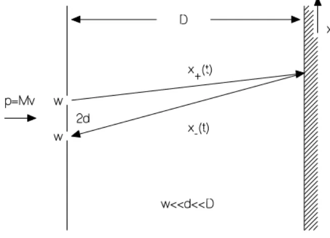
FIG. 1: Two slit experiment.

These velocities do not commute

[v₊,v₋] =i~ R

M2, (13)

and it is thereby impossible to fix the velocities forward and backward in time as being identical. Note that Eq.(13) is sim-ilar to the usual commutation relations for the quantum

veloc-itiesv= (p₋(eA/c))/M of a charged particle moving in a

magnetic fieldB; i.e.[v1,v2] = (i~eB3/M2c). Just as the

mag-netic fieldBinduces a Aharonov-Bohm phase interference for

the charged particle, the Brownian motion friction coefficient

Rinduces a closely analogous phase interference between

for-ward and backfor-ward motion which expresses itself as mechan-ical damping. Eq. (13) has been also discussed in connection with non-commutative geometry in ref.[25]: there it is shown that quantum dissipation induces in the plane of the forward and backward motion a non-commutative geometry.

Let me go now to consider the two-slit diffraction experi-ment (Fig. 1).

In order to derive the diffraction pattern one needs to know

the wave functionψ0(x)of the particle at time zero when it

“passes through the slits”, or equivalently the density matrix

(x+|ρ0|x−) =ψ0∗(x−)ψ0(x+). (14)

One wishes to find the probability density for the electron

to be found at positionxat the detector screen at a latter time

t,

P(x,t) = (x_|ρ(t)|x) =ψ∗(x,t)ψ(x,t), (15) in terms of the solution to the free particle Schr¨odinger equa-tion which is

ψ(x,t) =³ M

2π~it

´1/2Z ∞

−∞e [i

~A(x−x′,t)]_ψ

0(x′)dx′, (16)

where

A(x₋x′,t) =M(x−x′) 2

2t (17)

is the Hamilton-Jacobi action for a classical free particle to

move fromx′toxin a timet. Eqs.(14)-(17) imply that

P(x,t) = (18)

M

2π~t

Z ∞

−∞

Z ∞

−∞e

·

iM(x−x+)2₂−~t(x−x−)2

¸

(x+|ρ0|x−)dx+dx−.

Then Eq.(18) clearly shows that, werex+andx−always the

same, thenP(x,t)not oscillate inx, i.e. there would not be

the usual quantum diffraction. What is required for quan-tum interference in Eq.(18) is that the forward in time

ac-tion A(x₋x₊,t) differs from the backward in time action

A(x₋x₋,t): The quantum nature of the phenomenon is

cru-cially determined by the non-trivial dependence of the density

matrix(x+|ρ0|x−)when the electron “passes through the slits”

on the difference(x+−x−).

In the usual quantum diffraction experiment one considers

w_≪d _≪D, wherew is the opening of the slits which are

separated by a distance 2d, andDis the distance between the

slits and the screen where the diffraction pattern is observed (see Fig.1). Then the diffraction pattern is well described by

|x_{| ≫ |}x_±_|. By definingK=Mvd

~_D, β=

w

d, withv=D/t the

velocity of the incident electron, Eq.(18) leads [21] to the con-ventional result

P(x,D)≈_πβ4_Kx₂ cos2(Kx)sin2(βKx). (19) In obtaining (19) the initial wave function

ψ0(x) =

1

√

2

h

φ(x₋d) +φ(x+d)i, (20)

withφ(x) =√1_w if|x_{| ≤} w₂ and zero otherwise, has been used.

Eqs.(14) and (20) imply that

(x+|ρ0|x−) = (21)

1 2

n

φ(x₊₋d)φ(x₋₋d) +φ(x₊+d)φ(x₋+d) +φ(x+−d)φ(x−+d) +φ(x++d)φ(x−−d)

o .

If one accepts the notion of both forward in time and backward in time Hilbert spaces, then the following physical picture of two slit diffraction emerges. The particle can go forward and backward in time through slit 1 (this is described by the first term in the rhs of Eq.(21)). This is a classical process. The particle can go forward in time and backward in time through

slit 2, which is also classical since for classical casesx+(t) =

x₋(t)(the second term in the rhs of Eq.(21)). On the other

hand, the particle can go forward in time through slit 1 and backward in time through slit 2 (the third term), or forward in time through slit 2 and backward in time through slit 1 (the fourth term). These are the source for quantum interference since|x+(t)−x−(t)|>0.

In conclusion, by following Schwinger [23], it appears

(4)

(x+(t),x−(t)). A system acts in a classical fashion if the

two paths can be identified, i.e. xclassical(t)≡x+classical(t)≡

x₋_classical(t). When the system moves so that the forward in time and backward in time motions are (at the same time)

unequalx+(t)6=x−(t), then the system is behaving in a

quan-tum mechanical fashion and exhibits interference patterns in

measured position probability densities. Of course whenxis

actually measured there is only oneclassical x=x₊=x₋.

So far I have considered the low temperature limit, which

meansT_≪TγwherekBTγ=~γ=₂~_MR. In the high temperature

regimeT _≫T_γ, the thermal bath motion suppresses the

prob-ability forx+6=x−due to the thermal term(kBT R/~)(x+−

x₋)2_{in Eq.(8) (cf. also Eq. (11)). By writing the diffusion}

coefficientD=kBT

R as

D= T T_γ

³ ~

2M

´

, (22)

the condition for classical Brownian motion for high mass

par-ticles is thatD_≫(~_/₂M), and the condition for quantum

in-terference with low mass particles is thatD_≪(~_/₂M). For

large particles in, say, colloidal systems classical Brownian motion would appear to dominate the motion. For a single

atom in a fluid at room temperature it is typicallyD_∼(~_/₂M),

equivalentlyT _∼Tγso that quantum mechanics plays an

im-portant but perhaps not dominant role in the Brownian motion. Coordinate doubling has also entered into the canonical quantization of dissipative systems [15, 26, 27] and it appears to be intimately related to the algebraic properties of the the-ory [10, 12, 13, 28], as I will discuss below.

It is also interesting to note that the “negative” kine-matic term in the Hamiltonian (9) also appears in two-dimensional gravity models leading to two different strate-gies in the quantization method [29]: the Schr¨odinger repre-sentation approach, where no negative norm appears, and the string/conformal field theory approach where negative norm states arise as in Gupta-Bleurer electrodynamics.

In the following I will consider the algebraic structure of the space of the physical states emergent from the doubling of the degrees of freedom discussed in the present section.

III. THE DEFORMED HOPF ALGEBRA IN QFT

The study of several problems of physical interest where the doubling of the degrees of freedom has proved to play a crucial role in the canonical formalism has suggested, in recent years, that the structure of the state space in QFT is intimately related [12, 13] to the one of the deformed Hopf algebra [8, 9].

As already observed in the previous Section, the additivity of angular momentum, and of other so-called primitive oper-ators, such as energy and momentum, necessarily implies the use of the coproduct operation, a key ingredient of Hopf

alge-bras, defined by∆

O

=

O

⊗1+1_⊗

O

≡

O1

+

O2

, with

O

∈

A

,

which is a homomorphism which indeed duplicates the

alge-bra,∆:

A

→

A

⊗

A

. Since additivity of observables is an

es-sential requirement, Lie-Hopf algebra thus appears to be the

essential algebraic structure of QM and of QFT. A remarkable result is that the infinitely many uir of the ccr, whose existence

characterizes QFT, are classified by use of thedeformedHopf

algebra. Quantum deformations of Hopf algebra have thus a deeply non-trivial physical meaning in QFT. One can indeed show[12, 13] that the Bogolubov transformations

A(θ)≡√1

2(α(θ) +β(θ)) = Acoshθ−B

†

sinhθ (23)

B(θ)≡√1

2(α(θ)−β(θ)) = Bcoshθ−A

†

sinhθ (24)

are directly obtained by use of theq-deformed copodruct

op-eration:

∆aq=a1q1/2+q−1/2a2, ∆a†q=a

†

1q1/2+q−1/2a †

2. (25)

In Eqs. (23) and (24)α(θ) andβ(θ) are convenient linear

combinations [12, 13] of the coproduct operators (25) with the

deformation parameterq=e2θ. Note that[ai,aj] = [ai,a†j] =

0, i,j=1,2, i₆=jand[A(θ),A†_{(θ)] =}₁_, _[_B_(θ)_,_B†_{(θ)] =}₁

and all other commutators equal to zero. A(θ)andB(θ)also

commute. The momentum suffixκis omitted for simplicity.

Note that theAandB(or a1anda2) operators play here the

role of the doubled degrees of freedom (x+andx−in the

pre-vious Section).

The generator of (23) and (24) is

G

_{≡ −}i(A†B†₋AB):

−i δ

δθA(θ) = [

G

,A(θ)], −i δ

δθB(θ) = [

G

,B(θ)], (26)

and h.c.. Thus p_θ_{≡ −}i δ

δθ can be regarded [12, 13] as the

momentum operator “conjugate” to the “degree of freedom”

θ. For an assigned fixed value ¯θ, it is

e(iθp¯ θ)_A_{(θ) =}_e(iθ¯G)_A_(θ)_e(−iθ¯G)₌_A_(θ₊_θ)¯ _, ₍₂₇₎

and similarly forB(θ).

In the case of time–dependent deformation parameter, the

Heisenberg equation forA(t,θ(t))is

−iA˙(t,θ(t)) =−iδ

δtA(t,θ(t))−i δθ

δt δ

δθA(t,θ(t)) =

[H,A(t,θ(t))] +δθ

δt[

G

,A(t,θ(t))] = [H+Q,A(t,θ(t))], (28)

andQ_≡δθ

δt

G

plays the role of the heat–term in dissipative

systems.His the Hamiltonian responsible for the time

varia-tion in the explicit time dependence ofA(t,θ(t)). H+Qcan

be therefore identified with the free energy [15]: variations in time of the deformation parameter involve dissipation. In thermal theories and in dissipative systems the doubled modes

Bplay the role of the thermal bath or environment.

Let|0i ≡ |0i ⊗ |0idenote the vacuum annihilated byAand

B,A_|0i=0=B_|0i. By introducing the suffixκ, at finite

vol-umeV one obtains

|0(θ)i=e(i∑κθκGκ)_|₀_i₌

_∏

k

1

coshθk

e

³

tanhθkA†kB

†

k

´

(5)

θdenotes the set{θκ=1₂lnqκ,∀κ}andh0(θ)|0(θ)i=1.

The vacuum |0(θ)i is an SU(1,1) generalized coherent

state [30] (the group structure actually isN_κSU(1,1)κ):

co-herence and the vacuum structure in QFT are thus intrinsically

related to the deformed Hopf algebra. In the following

H

θwill

denote the Hilbert space with vacuum|0(θ)i:

H

θ≡ {|0(θ)i}.

In view of the similarity of some features of the coherent states with those of the fractals, it is an interesting question to ask whether fractal properties enter the QFT structure. A study on this point is in progress.

In the infinite volume limit, the number of degrees of freedom becomes uncountable infinite, hence one obtains

[7, 11, 15] h0(θ)|0(θ′₎_{i →}₀ _as _V _→_∞_, _∀_θ_,_θ′_, _θ₆₌_θ′_,

which means that the Hilbert spaces

H

θand

H

θ′ become

uni-tarily inequivalent. In this limit, the “points” of the space

H

≡ {

H

θ, ∀θ} of the infinitely many uir of the ccr are

la-belled by the deformation parameterθ[12, 13, 15].

Since QFT is characterized by the existence of uir of the ccr [5], and since these uir are related among themselves by the Bogoliubov transformations, which, as seen above are obtained as linear combinations of the deformed coproduct maps, we see that the doubling of the degrees of freedom is a general feature of QFT (independent of the specificity of the system under study) and that the intrinsic algebraic structure of QFT is thus the one of the deformed Hopf algebra. The uir existing in QFT are related and labelled by means of such a algebraic structure.

It should be stressed that the coproduct map is also essen-tial in QM in order to deal with a many modes system (typ-ically, with identical particles). However, in QM all the rep-resentations of the ccr are unitarily equivalent and therefore the Bogoliubov transformations induce unitary transforma-tions among the representatransforma-tions, thus preserving their physical content. The deformed Hopf algebra therefore does not have that physical relevance in QM, which it has, on the contrary, in QFT. Here, the representations of the ccr, related through

Bo-goliubov representations, are unitarilyinequivalentand

there-fore physically inequivalent: they represent different physical phases of the system corresponding to different boundary con-ditions, such as, for example, the system temperature. Typical examples are the superconducting and the normal phase, the ferromagnetic and the non-magnetic (i.e. zero magnetization) phase, the crystal and the gaseous phase, etc.. The physical

meaning of the deformation parameterqin terms of which uir

are labelled is thus recognized.

When the above discussion is applied to non-equilibrium thermal field theories it appears that the couple of

“ther-mal” conjugate variablesθandpθ≡ −i_∂θ∂, withθ=θ(β(t))

(β(t) = 1

kBT(t)), related to the q–deformation parameter,

de-scribe trajectories in the space

H

of the representations, i.e.

the space whose “points” are the uir of the ccr [12, 13]. In [10] it has been shown that there is a symplectic structure

as-sociated to the “thermal degrees of freedom”θand that the

tra-jectories in the

H

space may exhibit some properties typical

of chaotic trajectories in classical nonlinear dynamics. Such a

picture of a classical nonlinear dynamics in the space

H

of the

representations is not limited to thermal field theory, but it is a general feature of QFT. We will discuss this in the following.

In the next Section we present further characterizations of the vacuum structure of the uir in QFT.

IV. ENTANGLEMENT AND ENTROPY

The state|0(θ)iin Eq. (29) can be written as

|0(θ)i= Ã

∏

k

1

coshθk

!

(30)

×

Ã

|0i ⊗ |0i+

_∑

k

tanhθk(|Aki ⊗ |Bki) +. . . !

,

which clearly cannot be factorized into the product of two single-mode states. There is thus entanglement between the

modesAandBand|0(θ)iis an entangled state.

The state|0(θ)imay be also written as:

|0(θ)i=exp

µ

−1

2SA

¶

|

I

i=exp

µ

−1

2SB

¶

|

I

i, (31)

SA≡ −

∑

κ

n

A†_κAκln sinh2θκ−AκA†κln cosh2θκ o

. (32)

In these equations|

I

i ≡exp³∑κA†κB†κ ´

|0iandSBis given by

an expression similar toSA, withBκandB†κreplacingAκand

A†κ, respectively. I simply writeS for eitherSAor SB. I can

also write[7, 11, 15]:

|0(θ)_i=

+∞

∑

n=0 √

Wn(|n_{i ⊗ |}n_i), (33)

Wn=

∏

k

sinh2nk_θ k

cosh2(nk+1)θk

, (34)

with n denoting the set {nκ} and with 0<Wn <1 and

∑+n=∞0Wn=1. Then

h0(θ)|SA|0(θ)i=

+∞

∑

n=0

WnlnWn, (35)

and thusScan be interpreted as the entropy operator [7, 11,

15] and it provides a measure of the degree of entanglement. I remark that the entanglement is truly realized in the infinite volume limit where

h0(θ)|0i=e− V

(2π)3 R

d3κln coshθκ

−→

V→∞0, (36)

providedRd3κln coshθκis not identically zero. The

probabil-ity of having the component state|n_i⊗|n_iin the state|0(θ)iis

Wn. SinceWnis a decreasing monotonic function ofn, the

con-tribution of the states|n_{i ⊗ |}n_iwould be suppressed for large

nat finite volume. In that case, the transformation induced by

the unitary operatorG−1(θ)≡exp(−i∑κθκ

G

κ)could

(6)

the infinite volume limit, where the summation extends to an infinite number of components and Eq. (36) holds (in such a

limit Eq. (29) is only a formal relation sinceG−1_(θ)_{does not}

exist as a unitary operator)[18].

It is interesting to note that, although the modeBis related

with quantum noise effects, nevertheless theA₋B

entangle-ment is not affected by such noise effects. The robustness of the entanglement is rooted in the fact that, once the infinite volume limit is reached, there is no unitary generator able to

disentangle theA₋Bcoupling.

V. TRAJECTORIES IN THEH SPACE

In this Section I want to discuss the chaotic behavior, under

certain conditions, of the trajectories in the

H

space.

Let me start by recalling some of the features of the

SU(1,1)group structure (see, e.g., [30]).

SU(1,1)realized onC_×Cconsists of all unimodular 2×

2 matrices leaving invariant the Hermitian form|z_1|2_{− |}z_2|2,

zi∈C,i=1,2. The complex z plane is foliated under the

group action into three orbits: X₊={z:|z_|<1},X₋={z:

|z_|>1}andX0={z:|z|=1}.

The unit circleX₊={ζ:|ζ|<1},ζ≡eiφtanhθ, is

isomor-phic to the upper sheet of the hyperboloid which is the setH

of pseudo-Euclidean bounded (unit norm) vectorsn:n_·n=1.

His a K¨ahlerian manifold with metrics

ds2=4∂

2_F ∂ζ∂ζ¯dζ·d

¯

ζ, (37)

and

F_{≡ −}ln(1− |ζ|2) (38) is the K¨ahlerian potential. The metrics is invariant under the group action [30].

The K¨ahlerian manifoldHis known to have a symplectic

structure. It may be thus considered as the phase space for the classical dynamics generated by the group action [30].

TheSU(1,1)generalized coherent states are recognized to

be “points” inHand transitions among these points induced

by the group action are therefore classical trajectories [30]

inH(a similar situation occurs [30] in theSU(2)(fermion)

case).

Summarizing, the space of the unitarily inequivalent repre-sentations of the ccr, which, as seen in Section III, is the space

of the SU(1,1) generalized coherent states, is a K¨ahlerian

manifold,

H

_{≡ {}

H

θ, ∀θ_{} ≈}H; it has a symplectic structure

and a classical dynamics is established on it by theSU(1,1)

action (generated by

G

or, equivalently, by pθ:

H

θ→

H

θ′).

Trajectories in

H

describe transitions through the

representa-tions

H

θ={|0(θ)i}as theθ–parameter changes, i.e. through

the physical phases of the system, the system order parameter

being dependent onθ. One may then assume time-dependent

θ: θ=θ(t). For example, this is the case of dissipative

systems and of non-equilibrium thermal field theories where

θκ=θκ(β(t)), withβ(t) =_k 1

BT(t).

It is interesting to observe that, considering the transitions

H

θ→

H

θ′, i.e.|0(θ)i → |0(θ′)i, we have

h0(θ)|0(θ′)i=e− V

2(2π)3 R

d3_κF_κ(_θ_,_θ′₎

(39)

whereFκ(θ,θ′)is given by Eq. (38) with|ζκ|2=tanh2(θκ−

θ′

κ), which shows the role played by the K¨ahlerian potential

in the motion over

H

.

The result that the group action induces classical

trajecto-ries in

H

has been also obtained elsewhere [31, 32] on the

ground of more phenomenological considerations.

With reference to the discussion presented in Section II,

we may say that on the (classical) trajectories in

H

it is

x+=x−=xclassical, i.e. on these trajectories the quantum

noise accounted for byyis fully shielded by the thermal bath

(cf. Eq. (11)). In [20] it has been indeed shown that they

free-dom contributes to the imaginary part of the action which be-comes negligible in the classical regime, but is relevant for the

quantum dynamics, namely in each of the “points” in

H

(the

spaces

H

θ) through which the trajectory goes asθchanges.

Upon “freezing” the action ofG(θ)(i.e. upon “freezing” the

“motion” through the uir) the quantum features of

H

θ, at given

θ, become manifest. We thus recover ’t Hooft picture and the

results of ref. [2].

Let me use the notation|0(t)iθ≡ |0(θ(t))i. For anyθ(t) =

{θκ(t),∀κ}it is

θh0(t)|0(t)iθ=1, ∀t. (40)

I will now restrict the discussion to the case in which, for any

κ,θκ(t)is a growing function of time and

θ(t)6=θ(t′), ∀t₆=t′, and θ(t)6=θ′(t′), ∀t,t′. (41)

Under such conditions the trajectories in

H

satisfy the

re-quirements for chaotic behavior in classical nonlinear dynam-ics. These requirements are the following [33]:

i) the trajectories are bounded and each trajectory does not intersect itself.

ii) trajectories specified by different initial conditions do not intersect.

iii) trajectories of different initial conditions are diverging trajectories.

Let t0=0 be the initial time. The ”initial condition”

of the trajectory is then specified by the θ(0)-set, θ(0) =

{θκ(0),∀κ}. One obtains

θh0(t)|0(t′)iθ−→

V→∞0, ∀t,t

′_, _with _t₆₌_t′_, ₍₄₂₎

providedRd3κln cosh(θκ(t)−θκ(t′))is finite and positive for

anyt₆=t′.

Eq. (42) expresses the unitary inequivalence of the states

|0(t)iθ(and of the associated Hilbert spaces{|0(t)iθ}) at

dif-ferent time valuest ₆=t′ in the infinite volume limit. The

non-unitarity of time evolution implied for example by the damping is consistently recovered in the unitary inequivalence

among representations{|0(t)iθ}’s at differentt’s in the

infi-nite volume limit.

(7)

(the state vectors at timet) in

H

is finite (and equal to one)

for eacht. Eq. (40) rests on the invariance of the Hermitian

form |z_1|2_{− |}_z_2|2_, _z

i ∈C,i=1,2 and I also recall that the

manifold of points representing the coherent states |0(t)iθ

for any t is isomorphic to the product of circles of radius

rκ2=tanh2(θκ(t))for anyκ.

Eq. (42) expresses the fact that the trajectory does not crosses itself as time evolves (it is not a periodic trajectory):

the “points” {|0(t)iθ} and{|0(t′)iθ} through which the

tra-jectory goes, for anytandt′, witht₆=t′, after the initial time

t0=0, never coincide. The requirementi)is thus satisfied.

In the infinite volume limit, we also have

θh0(t)|0(t′)iθ′−→

V→∞0 ∀t,t

′ _, _∀_θ₆₌_θ′_. ₍₄₃₎

Under the assumption (41), Eq. (43) is true also fort=t′. The

meaning of Eqs. (43) is that trajectories specified by different

initial conditions θ(0)6=θ′(0)never cross each other. The

requirement ii) is thus satisfied.

In order to study how the “distance” between trajectories in

the space

H

behaves as time evolves, consider two trajectories

of slightly different initial conditions, sayθ′₍₀_{) =}_θ(₀_{) +}_δθ_,

with smallδθ. A difference between the states|0(t)iθ and

|0(t)iθ′ is the one between the respective expectation values

of the number operatorA†κAκ. For anyκat any givent, it is

∆

N

Aκ(t)≡

N

′Aκ

¡ θ′(t)¢

−

N

Aκ

¡ θ(t)¢

=θ′h0(t)|A†_κAκ|0(t)iθ′−θh0(t)|Aκ†Aκ|0(t)iθ (44)

=sinh2¡θ′κ(t)¢−sinh2¡θκ(t)¢=sinh¡2θκ(t)¢δθκ(t),

whereδθκ(t)≡θ′κ(t)−θκ(t)is assumed to be greater than

zero, and the last equality holds for “small”δθκ(t)for anyκ

at any givent. By assuming that∂δθκ

∂t has negligible variations

in time, the time-derivative gives

∂

∂t∆

N

Aκ(t) =2 ∂θκ(t)

∂t cosh ¡

2θκ(t)¢δθκ. (45)

This shows that, provided θκ(t) is a growing function of

t, small variations in the initial conditions lead to growing

in time ∆

N

Aκ(t), namely to diverging trajectories as time

evolves.

In the assumed hypothesis, at enough largetthe divergence

is dominated by exp(2θκ(t)). For eachκ, the quantity 2θκ(t)

could be thus thought to play the role similar to the one of the Lyapunov exponent.

Since [15]∑κEκ

N

˙Aκdt=β1dSA, whereEκis the energy of

the modeAκ, dSA is the entropy variation associated to the

modesAand ˙

N

Aκ denotes the time derivative of

N

Aκ, the

di-vergence of trajectories of different initial conditions may be expressed in terms of differences in the variations of the en-tropy (cf. Eqs. (44) and (45)):

∆

_∑

κ

E_κ

N

˙Aκ(t)dt=

1

β ¡

dS′_A₋dSA¢. (46)

The discussion above thus shows that also the requirement

iii) is satisfied. The conclusion is that trajectories in the

H

space exhibit, under the condition (41) and withθ(t)a

grow-ing function of time, properties typical of the chaotic behavior in classical nonlinear dynamics.

VI. CONCLUSIONS

Doubling the system degrees of freedom plays a crucial role in QM and QFT. The doubled degrees of freedom de-scribe the thermal bath or environment degrees and are en-tangled with the system degrees of freedom. They also ac-count for quantum noise in the fluctuating random forces in the system–environment coupling. The algebraic structure of QM and QFT is characterized and generated by the doubling of the degrees of freedom and is the one of the Hopf

alge-bra. Theq-deformed Hopf algebra allows the labelling of the

infinitely many unitarily inequivalent representations of the canonical (anti-)commutation relations existing in Quantum Field Theory and, by means of the Bogoliubov transforma-tions constructed by use of the deformed coproduct operation, transitions among the unitarily inequivalent representations are implemented. These transitions describe the processes of (both quantum and thermal) phase transitions in Quantum Field Theory. The transitions are described by trajectories in the space of the unitarily inequivalent representations, which turns out to be a K¨ahlerian manifold. These trajectory are classical trajectories which under convenient conditions may be chaotic trajectories. In this way we recognize that the clas-sical evolution along these trajectories is naturally embedded in the quantum frame of QFT.

VII. ACKNOWLEDGEMENTS

I acknowledge partial financial support from Miur, INFN, INFM and COSLAB.

[1] G. ’t Hooft, arXiv:hep-th/0003005.

G. ’t Hooft, Int. J. Theor. Phys., 42(2003) 355. G. ’t Hooft, arXiv:hep-th/0105105.

[2] M. Blasone, P. Jizba and G. Vitiello, Phys. Lett., A 287(2001) 205.

[3] M. Blasone, E. Celeghini, P. Jizba and G. Vitiello, Phys. Lett.,

A 310(2003) 393.

[4] H.T. Elze and O. Schipper, Phys. Rev.,66(2002) 044020. [5] O. Bratteli and D. W. Robinson, Operator Algebras and

Quan-tum Statistical Mechanics (Springer, Berlin, 1979).

(8)

[7] H. Umezawa, Advanced field theory: micro, macro and thermal concepts (AIP, N.Y. 1993).

U. Umezawa, M. Matsumoto and M. Tachiki, Thermo Field Dynamics and Condensed States (North-Holland, Amsterdam, 1982)

[8] V. G. Drinfeld, in Proc. ICM Berkeley, CA, ed. by A. M. Glea-son (AMS, Providence, R.I., 1986), 798p.

M. Jimbo, Int. J. Mod. Phys.,A 4(1989) 3759.

Yu. I. Manin, Quantum groups and Non-Commutative Geome-try (CRM, Montreal, 1988).

[9] E. Celeghini, T. D. Palev and M. Tarlini, Mod. Phys. Lett.,B5 (1991) 187.

P. P. Kulish and N. Y. Reshetikhin, Lett. Math. Phys.,18(1989) 143.

[10] G. Vitiello, Int. J. Mod. Phys., B 18(2004) 785.

[11] Y. Takahashi and H. Umezawa, Collective Phenomena2(1975) 55; reprint in Int. J. Mod. Phys.B10(1996) 1599.

[12] E. Celeghini, S. De Martino, S. De Siena, A. Iorio, M. Rasetti and G. Vitiello, Phys. Lett., A244(1998) 455.

[13] S. De Martino, S. De Siena and G. Vitiello, Int. J. Mod. Phys., BB 10(1996) 1615.

[14] E. Celeghini, S. De Martino, S. De Siena, M. Rasetti and G. Vi-tiello, Annals Phys., 241(1995) 50.

[15] E. Celeghini, M. Rasetti and G. Vitiello, Annals Phys., 215 (1992) 156.

[16] M. Martellini, P. Sodano and G. Vitiello, Nuovo Cim., A 48 (1978) 341.

[17] A. Iorio, G. Lambiase and G. Vitiello, Annals Phys.294(2001) 234.

[18] A. Iorio, G. Lambiase and G. Vitiello, Annals Phys.309(2004) 151.

[19] M.Blasone, P.Jizba and G. Vitiello, in Decoherence and Entropy

in complex systems, Lecture Notes in Physics, ed. by H.T. Elze (Springer 2004) p.151, [arXiv:quant-ph/0301031].

[20] Y. N. Srivastava, G. Vitiello and A. Widom, Annals Phys., 238 (1995) 200.

[21] M. Blasone, Y. N. Srivastava, G. Vitiello and A. Widom, Annals Phys., 267(1998) 61,

[22] R. P. Feynman, Statistical Mechanics (W. A. Benjamin Publ. Co., Reading, Ma. 1972)

[23] J. Schwinger, J. Math. Phys., 2(1961) 407.

[24] R. P. Feynman and F. L. Vernon, Annals of Phys., 24(1963) 118 .

[25] S. Sivasubramanian, Y.N. Srivastava, G. Vitiello, A. Widom, Phys. Lett.,A 311(2003) 97,

[26] H. Feshbach and Y. Tikochinsky, Trans. New York Acad. Sci., (Ser.II)38(1977) 44.

[27] M. Blasone, E. Graziano, O. K. Pashaev and G. Vitiello, Annals Phys., 252(1996) 115.

[28] G. Vitiello, Quantum dissipation and coherence, in Quantum-like models and coherent effects, ed. by R.Fedele and P.K.Shukla (World Scientific Publ. Co. Singapore 1995) p. 136, [arXiv:hep-th/9503135].

[29] R. Jackiw, Two lectures on two-dimensional gravity, gr-qc/9511048; D. Cangemi, R. Jackiw and B. Zwiebach, Annals of Phys.,245(1996) 408.

[30] A. Perelomov, Generalized Coherent States and Their Applica-tions (Springer, Berlin, 1986).

[31] R. Manka, J. Kuczynski and G. Vitiello, Nucl. Phys., B 276 (1986) 533.

[32] E. Del Giudice, R. Manka, M. Milani and G. Vitiello, Phys. Lett., A 206(1988) 661.