M. Krajnc Alves
Universidade Federal de Santa Catarina Departamento de Engenharia Mecânica Campus Trindade 88010-970 Florianópolis, SC. Brazil [email protected]
R. Rossi
Universidade de Caxias do Sul Departamento de Engenharia Mecânica Cidade Universitária 95070-560 Caxias do Sul, RS. Brazil [email protected]
An Extension of the Partition of Unity
Finite Element Method
Here, we propose an extension of the Partition of Unit Finite Element Method (PUFEM) and a numerical procedure for the solution of J2 plasticity problems. The proposed method is based in the Moving Least Square Approximation (MLSA) and is capable of overcoming singularity problems, in the global shape functions, resulting from the consideration of linear or higher order base functions, in the classical PUFEM. The classical PUFEM employs a single constant base function and results in the so-called Sheppard functions. In order to avoid the presence of singular points, the method considers an extension of the support of the classical PUFEM weight function. Moreover, by using a single constant base function, the proposed method reduces in the limit, to the classical PUFEM. Since the support of the global shape functions do overlap, the method becomes closely related to the Element Free Galerkin (EFG) method. The most important characteristic of the proposed method is that it can be naturally combined with the EFG method allowing us to impose, in some limiting sense, the essential boundary conditions, avoiding the usage of the penalty and/or multiplier methods. In order to obtain higher order global shape functions a hierarchical enhancement procedure was implemented.
Keywords: PUFEM, EFG, MLSA and plasticity
Introduction
In the last years some new numerical methods have being used to solve classic boundary value problems in mechanics. These methods are called in the literature as meshless or mesh-free methods. Among them we could cite the Element Free Galerkin (EFG) (Belytschko et al, 1994), hp Clouds (Duarte and Oden, 1995), and Partition of Unit Finite Element Method (PUFEM) (Melenk and Babuska, 1996). Each of them, according with cited authors, has some advantages upon the traditional numerical methods. Such advantages can be described as the independence, at least in some aspects, of the mesh, the possibility to work with approximation spaces that include a-priori additional information of the PDE solution base, and the facility of implementing “p” enrichment strategies. Such behaviors allow the usage of these new methods in problems that traditional methods like the Finite Element Method (FEM) have encountered some difficulties to solve. Problems of large deformation, crack growth, adaptive approaches among others are examples of its applications.1
Naturally, together with these new methods, new problems have appeared, such as: the determination of appropriate numeric integration scheme, the development of new data management procedures, the increase in the computational cost when compared with the traditional FEM, the difficulty to the impose the essential boundary conditions, and the occurrence of stability problems associated with the use of a hierarchical enhancement procedure among others.
In this work we derive an extension of the PUFEM based on the framework of the Moving Least Square Approximation (MLSA) that ensures the construction of invertible matrices involved with the MLSA method. Notice that, by employing a single constant base function we derive, in the framework of MLSA, the so-called Sheppard functions, which characterize the PUFEM. However, by considering a large initial base the so-called moment matrices, which are derived in the framework of MLSA, become singular at some points in the support of the global shape function, as will be shown after. To overcome this problems we introduce a slightly perturbation of the support of the weight functions. Another important problem occurs when we consider the addition of hierarchical functions to the base approximations. Such hierarchical
Paper accepted June, 2005. Technical Editor: Atila P. Silva Freire.
enrichment, which can also be used in p-adaptive procedures, is responsible for some serious stability problems occurring in the solution procedure. Thus, care must be used when using such approach as seen in Taylor et al (1998). Here, we apply the proposed method for the solution of a J2 plasticity model which accounts for a non-linear isotropic and kinematic hardening law, see Lemaitre (1992). In order to integrate the local evolution equations and to derive the consistent tangent operator we consider the approach proposed by Benallal et al (1988). The derived algorithm belongs to the returning mapping class and has a quadratic convergence rate. Some plane stress examples are presented in order to show the evolution of the internal variables as well as the influence of usage of a uniform hierarchical enhancement.
The imposition of essential boundary conditions in meshless approximations is a problem of great concern. Different approaches have been presented in order to achieve this goal. Among the presented approaches are the ones which combine meshless methods with the finite element approach, as seen in Hegen (1996) and Krongauz and Belytschko (1996). However, these approaches require special procedures that are not simple to implement. Other approaches employ the penalty and/or multiplier methods, Duarte and Oden (1995), and the use of a singular weight function at nodes, see Kaljevic and Saigal (1997). At this point, it is important to notice that one of the main characteristic of the proposed extended PUFEM is its ability to be naturally incorporated into a meshless, or particularly the EFG, approximation procedure allowing us to impose, as close as desired, the essential boundary conditions. In this way we avoid not only the complexities of the implementation of the combined meshless with FEM approaches but also the usage of the penalty and/or multiplier methods. The penalty and/or multiplier methods may be applied in problems formulated in terms of saddle point formulations, which poses some restriction on the applicability of such methods to more general formulations, and require the introduction of additional terms when compared with the direct application of the Galerkin method using a base which comply, at least approximately, with the essential boundary conditions.
Moving Least Square Approximation – MLSA
solve some boundary value problems. Also, based on the MLSA we can derive the PUFEM by a proper selection of both the base and weight functions. The MLSA may be summarized, (see Lancaster and Salkauskas (1981)), as:
Consider a function u∈ Ω with a boundary ∂Ω, decomposed in a region ΓE where an essential boundary condition is prescribed
and in a region ΓN where a natural boundary condition is
prescribed. Both regions are such that ∂Ω = Γ ∪ ΓE N and
{ }
E N
Γ ∩ Γ = ∅ . An approximation h
u of u
( )
x may be obtainedby considering:
( )
( ) ( )
( ) ( )
1
m
h T
j j j
u p a
=
=
∑
⋅ =x x x p x a x . (1)
Here m is the number of terms in the base of functions used in the MLSA, for example m = 3 means T
[
1]
x y
=
p for Ω ∈2D
with T
[
,]
x y
=
x or 2
1
T
x x
⎡ ⎤
= ⎢⎣ ⎥⎦
p for Ω ∈1D, and a x
( )
is thevector whose components are the coefficients of the base functions that must be determined. The criteria enforced for the determination of the coefficients of a x
( )
is the minimization of the weighteddiscrete L2 norm given by:
( )
(
)
( ) ( )
2
1 1
n m
I k I k I
I k
J w p a u
= =
⎡ ⎤
⎢ ⎥
= − ⎢ ⋅ − ⎥
⎣ ⎦
∑
∑
a x x x x . (2)
Here, n represents the number of points in the neighbourhood of xfor which the weight function w
(
x−xI)
≠0, and uI is the nodalvalue of u
( )
x at xI. By minimizing J( )
a with relation to thecomponents of a x
( )
we derive( )
( )
1
n h
I I I
u u
=
=
∑
Φx x . (3)
Here
( )
T( ) ( )
1( )
I I
−
⎡ ⎤
Φ x =p x ⎣Α x⎦ D x (4)
where ΦI
( )
x is the global shape functions used in theapproximation procedure with
( )
(
) ( ) ( )
( )
(
) ( )
1
and
n
T
i i i I I I
i
w w
=
⎡ ⎤
=
∑
− ⎢⎣ ⎥⎦ = −Αx x x p x p x D x x x p x (5)
The matrix Α
( )
x is the so-called the moment matrix.PUFEM Derivation
The PUFEM may be obtained as a particular case of the EFG method, where we employ the MLSA. This is obtained by using, in the MLSA, a single constant base function and a classical FE base as the weighting function. As a result, by performing a partition of the domain, in triangular elements, we can determine a particular PUFEM approximation by employing as a weighting function the
classical linear triangular finite element base function (Tri3). In this particular case, the weight function may be explicitly written as
(
)
(
) (
) (
)
( )
(
)
1 1 1 1
1
, 1 1
2
for supp
0 otherwise
i i i i i i i i
I I
x y x y y y x x x y i k
A w
+ + + +
⎧⎪ ⎡ ⎤
⎪ − + − + − = −
⎪ ⎢⎣ ⎥⎦
⎪⎪ ⎪⎪⎪
− =⎨⎪ ∈ Φ
⎪⎪ ⎪⎪ ⎪⎪⎪⎩
x x x x
…
(6)
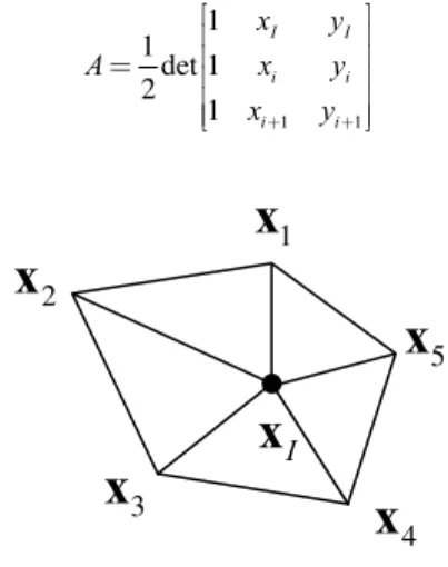
Here, k is the size of the adjoint node list, Fig. 1,
(
x yi, i)
are the components of the node xi and A is the cell area given by1 1
1 1
det 1 2
1
I I i i i i
x y
A x y
x+ y+
⎡ ⎤
⎢ ⎥
⎢ ⎥
= ⎢ ⎥
⎢ ⎥
⎢ ⎥
⎣ ⎦
(7)
Figure 1. PUFEM support function – supp (φI(X)).
In the literature those approximations that considers m=1 are known as Shepard approximations. In Sheppard´s case the global shape functions reduce to
[ ]
( )
(
)
(
)
1
1 1
1 n I I
i i
p w
w −
=
= → = ∴ = −
−
∑
A x D x x
x x
. (8)
Since,
(
)
1
1
n
i i
w =
− =
∑
x x , we have( )
T( ) ( )
1( )
(
)
I I w I
−
⎡ ⎤
Φ x =p x ⎣Α x⎦ D x = x−x . (9)
Thus, the use of this approach reproduces the traditional FEM. The use of the MLSA method enables us to improve the space of the approximation functions and reproduce polynomials of higher order. One way to achieve higher order polynomial approximations is to increase the size of the base p x
( )
by adding monomials.Unfortunately, this process leads to global shape functions that are undefined at some points of their support. This problem is a direct consequence of the singularity of the matrix Α
( )
x , defined inEq.(5), in a set of points. In order to identify these points we consider a point x that belongs to a generic triangular element (integration cell), of a typical support of a global shape function derived by using a classical linear finite element base function as the weight function for the MLSA, as illustrated in the Fig. 2.
I
x
5
x
1x
2
x
3
x
Figure 2. Typical support of the resulting global shape function.
Now, by restricting the base of the MLSA to m=3, i.e., for
[
1]
T
x y
=
p , we can derive at the point x the following
expression for the moment matrix Α
( )
x( )
(
) ( ) ( )
(
) ( ) ( )
(
) ( ) ( )
(
) ( ) ( )
3
1 1 1
1
2 2 2 3 3 3
T T
i i i i
T T
w w
w w
=
⎡ ⎤ ⎡ ⎤
= − ⎢⎣ ⎥⎦= − ⎢⎣ ⎥⎦+
⎡ ⎤ ⎡ ⎤
+ − ⎢⎣ ⎥⎦+ − ⎢⎣ ⎥⎦
∑
Α x x x p x p x x x p x p x
x x p x p x x x p x p x
(10)
Notice that, in this particular case, the full rank of Α
( )
xisrank⎡⎣A x
( )
⎤ =⎦ 3. Moreover, in order to determine the global shapefunctions ΦI
( )
x we must compute the inverse of Α( )
x . However,( )
Α x is singular at a set of points. These points can be easily identified once we observe that the weight functions do satisfy the property that, i.e., wI
( )
xj =w(
xj−xI)
=δIj, where xj is a node and wI( )
xj the weigh function. As a result, we verify:At x=xi→rank⎡⎣A x
( )
⎤⎦=1.Also by considering xi andxj, so that the segment joining
these points are parallel to the x/y global axis, we verify:
(
1 λ)
i λ j, with λ[ ]
0,1∈ − + ∈
x x x →rank⎡⎣A x
( )
⎤⎦=2.Moreover, even when more terms are added to the basis p x
( )
,the singularity ofΑ
( )
x is maintained at these points. In order toovercome these singularity problems, we propose the use of an extended PUFEM formulation.
PUFEM Extension Formulation
The main idea to avoid the singularity showed in the earlier section is to allow the PUFEM weight function to overlap its support by a given ε as ilustrated in Fig. 3. By the use of this approach we assure the influence of the neighborhood weight functions over those problematic points so that we can eliminate the singularity problems in the matrix Α
( )
x .Moreover, from the general properties of the MLSA, the global shape functions generated by this approach satisfies the partition of unity condition, i.e.,
( )
11
n I I=
Φ =
∑
x . (11)Figure 3. Extended PUFEM support – X*i is an extended node.
The extended points showed in Fig. 3 are determined as:
(
1)
, with 1i λ I λ i λ ε
∗= − + = +
x x x . (12)
Now, by taking ε→0, we derive global shape functions that satisfy, in the limit, the “Kronecker delta condition”, i.e.,
( )
0
lim i j ij
ε→ Φ x =δ , (13)
where xj is a node.
This implies that the essential boundary conditions can be imposed in the same way as in the traditional FEM provided we consider a sufficiently small value for ε. In the examples presented in this work we made use of 8
10
ε= −
. Therefore, for a finite ε, a small violation of the Kronecker delta condition occurs, i.e., of the essential boundary condition.
0 1 2 3 4 5 6
0 0 . 2 0 . 4 0 . 6 0 . 8 1
x
Φ 2 Φ 3 Φ 4 Φ 2 + Φ 3 + Φ 4
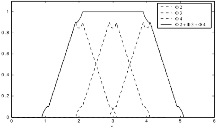
Figure 4. Global shape functions φI(x) in the one-dimensional case and the
partition of unity.
Some examples of one-dimensional shape functions, ΦI
( )
x ,generated by the extended PUFEM method, are shown in Fig.4. Notice that Φ2
( )
x represents a global shape function centered at x= 2. Moreover, the non-linearity seen near the nodes appears due to the overlapping of the weighting functions. It is important to point out that, in this example, we are using a very large perturbation0.1
ε= in order to magnify the perturbation effect over the final global shape functions. Notice that, the derived base functions define, in fact, a partition of unity.
3
x
1
x
2
x
x
I
x
5
x
∗ 1x
∗2
x
∗3
x
∗4
x
∗The extended PUFEM allow us to increase the polynomial approximation order by considering a larger base for p x
( )
.However, the resulting moment matrix Α
( )
x becomes large and thecost of determining its inverse becomes prohibitive. An alternate way to circumvent these high computational costs is to consider a hierarchical enhancement procedure.
Hierarchical Enhancement
According to the work of Taylor et al (1998) a hierarchical enhancement can be obtained using the following strategy
( )
n{
( )
}
h T
I I I I I
u x =
∑
Φ u +P x b , (14)where the vector P xI
( )
is a set of approximation functions, thattogether with the original basis ΦI will compose the final approximation space. The coefficients bI and uIare the
components of the approximation function and are determined by applying the Galerkin method. The advantage of this procedure is due to the reduced cost of computing the global shape function ΦI,
for a small base such as used in this work, i.e., m = 3 which means
[
1]
T
x y
=
p for Ω ⊂2D, and the increase of the polynomial
order with the addition of the new terms. In the work presented by Oden et al (1998) it is suggested that, to avoid linear dependency, we must not include elements from the space span
{
ΦI( )
x}
aselements of P xI
( )
. Moreover, we can mention that when onlypolynomials are used to compose P xI
( )
and p x( )
a carefulanalysis should be done in the final approximation form to avoid the stability problems identified with the addition of the new terms (see of Taylor et al (1998)).
(
) (
2)(
) (
)
2...
T
I =⎡⎣⎢ x−xI x−xI y−yI y−yI ⎤⎥⎦
P , (15)
Notice that, the hierarchical enhancement procedure is very simple to implement, when compared with the traditional FEM. However, the hierarchical procedure is considerably more expensive computationally than the traditional FEM, due to the large number of degrees of freedom generated per node.
Also, it is important to notice that, the increase in the polynomial approximation order by the consideration of a larger base for p x
( )
is limited in practice due to the prohibitive cost ofcomputing the inverse of the derived moment matrix Α
( )
x . On theother side, the usage of a hierarchical enhancement procedure is responsible for serious stability problems when determining the solution of the problem. These stability problems are associated with the quasi-linear dependence, of the base of the approximate solution space generated by the hierarchical enhancement procedure, at the integration points. Thus the resulting stiffness or tangent stiffness matrix is ill conditioned. This result is valid for all meshless methods. Thus, a compromise must be considered between both procedures. Notice that in the particular case of the EFG method, as proposed by Belytschko et al (1994), the importance of the proposed extended PUFEM with the objective of imposing the essential boundary condition is very well identified. One way to overcome the ill conditioned of the global matrix, associated with the derived linear system, when considering more terms in the hierarchical procedure, is to add to the global matrix a term of the
type αI, where I is the identity matrix and α is a sufficiently small positive scalar. The final solution is then determined by applying an iterative improvement of the solution, of the given linear system, by reducing the value of α.
Elastoplastic Model
Here, we make use of the elastoplastic model, proposed by Lemaitre (1992), which is derived in the framework of the thermodynamics of irreversible process. In this framework we postulate the existence of the Helmholtz specific free energy
( , , )e
r
Ψε α , where α is the backstrain tensor, r is the isotropic hardening strain measure, and εe
is the elastic part of the strain tensor ε. Now, considering the local state method and enforcing the Clausius-Duhem inequality we derive the following state equations:
, D and
e R
r
Ψ Ψ Ψ
= = =
σ χ
ε α
∂ ∂ ∂
ρ ρ ρ
∂ ∂ ∂ (16)
Here, ρ is the mass density; χD
is the deviatoric tensor associated with the back stress tensor χ, which is related to the kinematic hardening; and R is the isotropic hardening stress measure associated with the isotropic hardening. Moreover, the elastoplastic model considers the Helmholtz specific free energy potential to be given as:
1 1 1
( )
2 3
e e br
R r e
b −
∞ ∞
Ψ = Cε ε⋅ + + + α α⋅
ρ χ γ (17)
where, C is the forth order elasticity tensor and χ∞,R∞, b and γ are
material parameters associated with the hardening laws. Now, from Eq. (16) and Eq. (17) we derive the following state equations:
e
σ= Cε , (18)
for the elasticity equation;
(1 br)
R=R∞ −e− , (19)
for the isotropic hardening equation;
2 3
D
∞
=
χ χ γα, (20)
for the kinematic hardening equation.
Dissipation F
In order to describe the evolution of the dissipative process we postulate the existence of a pseudo-potential of dissipation which may be expressed as:
( , , D; , , ,)e
F=F σ Rχ ε rα (21).
The complementary equations can be derived from the pseudo-potential by applying the hypothesis of normal dissipation. This leads to the following expressions:
, and
p
D
F F F
r R
= = =
ε α
σ χ
∂ ∂ ∂
λ λ λ
Here, εp is the plastic strain rate and λ the plasticity multiplier rate.
In order define the pseudo-potential of dissipation; associated with the elastoplastic evolution laws, we introduce a yield criteria function, f. Here, we consider fto be given by:
y
( D D) 0
eq
f= σ −χ − −R σ = (23)
where
1
3 2
2
( D D) ( D D) ( D D)
eq ⎡ ⎤
− =⎢⎣ − ⋅ − ⎥⎦
σ χ σ χ σ χ and σy denotes the yield
stress.
At this point, we consider the pseudo-potential of dissipation, related to the elastoplastic evolution model, to be given as:
y 3
( )
4
D D D D
eq
F R
∞
= σ −χ − −σ + χ χ⋅
χ (24)
Now we derive, from Eq.(24), with the application of the hypothesis of normal dissipation, the following elastoplastic evolution laws:
• The plastic strain evolution law
3 ( )
2 ( )
D D p
D D eq
ε = −
−
σ χ
σ χ
λ
(25)
• The isotropic hardening evolution law
r=λ (26)
• The kinematic hardening evolution law
3 ( )
2 ( )
D D D D D eq ∞ ⎡ − ⎤ ⎢ ⎥ = ⎢ − ⎥ − ⎢ ⎥ ⎣ ⎦
σ χ χ
α
σ χ
λ
χ (27)
It is more convenient, however, to write Eq. (26) and Eq. (27) with respect to R and χD
respectively. This is done through the substitution of Eq. (26) and Eq. (27) into the time derivatives of Eq. (19) and Eq. (20). Then we derive:
• The isotropic hardening evolution law
( )
R=λb R∞−R (28)
• The kinematic hardening evolution law
( )
( )
D D D D D D eq ∞ ∞ ⎡ − ⎤ ⎢ ⎥ = ⎢ − ⎥ − ⎢ ⎥ ⎣ ⎦
σ χ χ
χ
σ χ
λχ γ
χ (29)
The determination of the plasticity multiplier rate λ is obtained by the enforcement of the consistency conditions, given by:
0 and 0
f= f= . Applying these conditions to the Eq. (23) and making use of the evolution laws we derive:
3 2 3 2 ( ) ( ) ( ) ( ) D D
D D D D D eq
b R R
∞ ∞ − ⋅ =⎡ ⎤ − − − ⋅ − ⎢ ⎥ ⎣ ⎦
σ χ σ
σ χ χ σ χ
λ
χ γ + γ . (30)
Here, we also define the accumulated plastic strain rate that is given by 1 2 2 3 p p
p=⎛⎜⎜⎜⎝ ⋅ ⎟⎞⎟⎟⎟
⎠
ε ε . (31)
Algorithm Description for the Global Equilibrium Equations
Let 2
R
Ω ⊂ be a bounded domain with a Lipschitz boundary ∂Ω, subjected to the boundary conditions σn=tatΓN -
prescribed surface traction and u=uatΓE - prescribed
displacement with ∂Ω = Γ ∪ ΓN E and Γ ∩ Γ = ∅N E . Let t denote a
loading parameter and f the prescribed body force. Then, by applying the Galerkin method, we can derive the weak formulation of the problem which is stated as: Given t, determine 1
( )
H
∈ Ω
u so
that
( )
1 0 ( ) ( ) , Nd d d H
Ω Ω Γ
⋅ Ω = ⋅ Ω + ⋅ Γ ∀ ∈ Ω
∫
σ u εv∫
f v∫
t v v (32)At this point, we can apply the extended PUFEM and obtain the global shape functions that define the approximation space. Let
1
n+
U denote the vector of nodal coefficients, associated with the approximating global shape functions, defined at the load parameter
1
n
t+ . Then, the discretized formulation of the problem may be
expressed as: Given tn+1, determine Un+1 so that
1 1 1
( n+)= e( n+)− i( n+)=
h U F U F U 0 (33)
Here, F Ue( n+1) and F Ui( n+1) are the discretized external and internal nodal load vector respectively. Now, by combining an incremental load procedure with Newton`s method we derive the following scheme:
(i) Initialize the trial solution by setting 0 1
n+ = n
U U , where Un is
the converged solution at load step tn,
(ii) While (error > tol) do • Solve for 1
i n+
∆U , at the i-th iteration, by solving
1 1 ( 1)
i i i n+∆ n+ = − n+
K U h U
• Determine new trial solution 11
i n
+ +
U by the following update procedure
1
1 1 1
i i i n n n
+
+ = ∆ + + +
U U U
• Compute the new error measure by
Error = 1
1 ( i )
n
+ +
h U
End while
Here, 1
1
1 ( i )
i n n i n + + +
= h U K
U ∂
∂ and may be expressed as
1 1
i T i
n+ n+ d
Ω
=
∫
ΩK B J B where B is the strain-displacement matrix
associated with the extended PUFEM global shape functions and
1
i n+
J is the tangent operator defined by the elastoplastic model.
Local Integration
With the objective of simplifying the description of the algorithm we introduce the vectors
( p, D, ) andR ( , , )
= =
defined in Eq.(25),(28) and (29), may be written in a compact form as
( , ) =
Q λGσQ (34)
Now, with the application of the generalized trapezoidal rule of integration we derive the following incremental evolution law:
( n+ , n+ )
∆ = ∆Q λGσ θ Q θ =0. (35)
Here, we define the following operators: ∆( )=( )n+1−( )n and ( )n+θ= −(1 θ)( )n+θ( )n+1 with θ 0,1∈
[ ]
.Algorithm
The proposed algorithm is based in the work of Benellal et al (1988), belongs to the general class of return mapping algorithms, and is described by the following procedure:
(i) Given εn+1, we assume a purely elastic increment. As a result, ∆ =Q 0, 0∆λ = and the resulting stress, denoted as the trial stress state, is computed as:
1
*
1 n
TR n+ = +
σ Cε (36)
where *
1 1
p n+ = n+ − n
ε ε ε . Here, p
n
ε is the plastic strain tensor determined at the load parameter tn.
(ii) With the trial stress defined in Eq.(36), we check the yield criteria function. If ( TR1, ) 0
n n
f σ + Q < then hypothesis (i) is correct and the local procedure is complete and only the stress components of qmust be updated, i.e., 1 TR1
n+ = n+
σ σ and Qn+1=Qn. However, if f(σn+1,Qn+1)≥0 then we must perform an elastoplastic correction.
(iii) In order to perform the plastic corrections, relative to the load parameter tn+1, we must enforce: the incremental law, in Eq.(35); the yield criteria; and the elastic constitutive equation. As a consequence we derive the following set of nonlinear equations:
1 1 1 1
2...4 1
1
5 1 1
( ) ( , ) 0
( ) ( , ) 0
( ) 0
n n n
n n n
e n n
g f
g
g
+ + +
+ + +
−
+ +
= =
= ∆ −∆ =
= − =
q σ Q
q Q G σ Q
q ε C σ
θ θ
λ (37)
where 1 1 1
e p
n+ = n+ − n+
ε ε ε .
The solution of the nonlinear system of equations, Eq.(37), may be achieved by the application of Newton’s method. In this case we obtain the following procedure:
(i) Initialize the trial solution 0
1 ( 1, ,0)
n+ = n+ n
q σ Q ,
(ii) While (error > tol) do: • Determination of 1
k n+
∆q , associated with the k-th iteration, by solving the system:
1 1 ( 1)
k k k n+∆ n+ = − n+
M q g q
• Computation of 1 1
k n
+ +
q by using the following update procedure 1
1 1 1
k k k n n n
+
+ = ∆ + + +
q q q
• Determination of the error measure
Error = 1
1( 1)
k n n
+
+ +
g q
End while
Here,
1
k n+1 K
n+
= g
M q ∂
∂ and g
( )
⋅ is a vector function whose components are composed by the scalar functions and the components of the vector and tension functions defined in Eq.(37).Tangent Operator 1
i n+
J
After the local integration algorithm has converged, the corresponding consistent operator associated with the discretization may be determined by letting all the variables q and εvary slightly around the solution at the converged solution at iteration n+1. Thus,
=
σ J ε
δ δ (38)
with
1
1 ( , , p, ( ) )
n n n n n
n
∂
∂
+
+
− =
=
σ σ ε ε εu ε
J
ε u u (39)
Now, in order to compute the above differentiation we must enforce the incremental evolution laws. As a result, we have for the i-th component that:
1 1
0
i i
j kl j n kl n
g g
q ε
q + ε +
⎡⎛⎜⎢ ⎞⎟ ⎛⎜ ⎞⎟ ⎤⎥
⎟ ⎟
⎜ ⎟ +⎜ =
⎢⎜⎜⎜ ⎟⎟⎟ ⎜⎜⎝ ⎟⎟⎟⎠ ⎥
⎢⎝ ⎠ ⎥
⎣ ⎦
∂ ∂
δ δ
∂ ∂ (40)
Examples
One-Dimensional Plane Stress Case
The Fig. 5 shows the one-dimensional body taken into account in this analysis. The body is submitted to a monotonic traction load
t . The materials properties used in this example are: σy = 520 MPa, χ∞= 200 MPa, R∞= 4305MPa, b = 0.2 and γ = 20.
For the monotonic one-dimensional case we can check exactly isotropic and kinematic hardening. The isotropic hardening must follow the Eq.(19), and we can show that the state, Eq.(20), reduces to:
(
1 e γεp)
χ χ −
∞
= − . (41)
Figure 5. One-dimensinal body discretization.
In the Fig. 6 we show the results obtained from the model described in the Fig. 5.
(a)
(b)
(c)
(d)
Figure 6. a) Analytical x Numerical hardening; b) loading history; c) accumulated plastic strain; d) stress-strain response.
Bi-Dimensional Plane Stress Case
The Fig. 7 shows the body used in bi-dimensional example. This body is under an axial monotonic load t as described in the figure.
The material parameters used in this example are the same given in the earlier one-dimensional case.
t
lines of simmetry
Figure 7. Body under uniaxial load.
The discretized model is constructed based on the lines of symmetry showed in the Fig. 7. The integration mesh used is displayed in the Fig. 8.
Figure 8. Integration mesh.
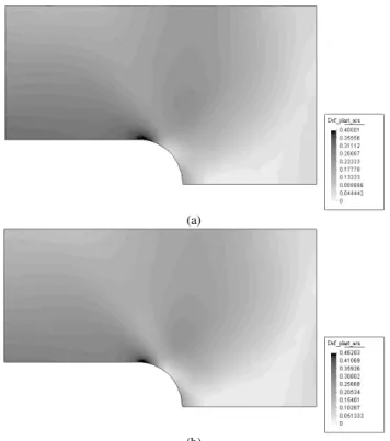
In the Fig. 9 are showed the results in a contour fill format for the accumulated plastic strain in the same time step.
(a)
(b)
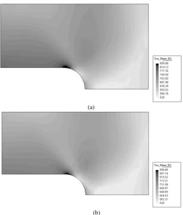
Figure 10 displays the contour fill results for the equivalent stress ( D D)
eq
−
σ χ in the same load step taken into account by the two different types of approximation.
(a)
(b)
Figure 10. Equivalent stress (σD - χD)eq - Comparison between a simple
global shape approximation (a) and hierarchical enhancement with completely quadratic monomials (b) at the same loading step.
Notice that, as expected, we observe an improved result for the hierarchical enhancement approach, with complete quadratic monomials, when compared with the one obtained by using a simple global shape approximation procedure. However, when the hierarchical enhancement is increased to include the complete cubic monomials, we experience instability problems. Thus, special procedures, as stated in the Hierarchical Enhancement section must be considered in order to cope with the instability problem.
Conclusions
In this work we proposed an extended Partition of Unity Finite Element Method that is able to overcome the singularity problems that arises in the determination of the global shape functions, when considering a large set of base functions in the MLSA framework. Moreover, the proposed method can be naturally combined with mesh-free methods, such as the EFG, allowing us to impose, as close as desired, the essential boundary condition avoiding the, some times questionable, usage of the penalty or the multiplier methods.
In order to attest the performance of the method we considered the solution of J2 plasticity problems. The method has shown to be very robust and efficient and the approximate enforcement of the essential boundary conditions to be very effective. Also, since the derived element tangent stiffness matrices are evaluated at the integration points that can be selected as interior points of the triangular integration cell, the resulting global tangent stiffness matrix is numerically well conditioned.
In order to increase the approximation space we have implemented a hierarchical enhancement procedure. An improvement of the results is verified as expected. However, we have observed some stability problems when considering the addition of cubic monomials. In order to circumvent this stability problem we must consider some special stabilization procedures as suggested in the Hierarchical Enhancement section. Thus, for an efficient usage of the method we need to make a compromise between the increase of the base of functions in the MLSA approach and the addition of higher order polynomial terms in the hierarchical enhancement procedure. Notice also that the proposed method allows, as is done in the EFGM, the consideration for example of special singular functions in the base of functions of the MLSA when determining stress intensity factors in fracture mechanical problems among others. This shows that the method can be applied to solve a large variety of mechanical problems in a very simple and effective way.
Acknowledgments
The support of the CNPq – Conselho Nacional de Desenvolvimento Científico e Tecnológico – is gratefully acknowledged.
References
Belytschko, T. and Fleming, M., 1999, “Smoothing, enrichment and contact in the element free galerkin method”, Computer and Structures, Vol. 71, pp. 173-195.
Belytschko, T., Krongauz, Y., Organ, D., Fleming, M. and Krysl P., 1996, “Meshless methods: An overview and recent developments”, Computer Methods in Applied Mechanics and Engineering, Vol.139, pp.3-47.
Belytschko, T., Lu, Y. Y. and Gu, L., 1994, “Element Free Galerkin Methods”, International Journal For Numerical Methods in Engineering, Vol. 37, pp.229-256.
Benallal, A., Billardon, R. and Doghri, I., 1988, “An Integration Algorithm and the Corresponding Consistent Tangent Operator for Fully Coupled Elastoplastic and Damage Equations”, Communications in Applied Numerical Methods, Vol. 4, pp.731-740.
Duarte, C.A. and Oden, J. T., 1995, “Hp-Clouds-a meshless method to solve boundary-value problems”, Technical Report 95-05, Texas Institute for Computational and Applied Mathematics, University of Texas at Austin.
Hegen,D., 1996, “Element-free Galerkin methods in combination with finite element approaches”, Comput. Methods Appl. Mech. Engrg., 135, pp143-166.
Kaljevic, I. and Saigal, S., 1997, “An Improved Element Free Galerkin Formulation, International Journal for Numerical Methods in Engineering, Vol. 40, pp.2953-2974.
Krongauz,Y. And Belytschko,T., 1996, “Enforcement of essential boundary conditions in meshless approximations using finite elements”, Compt. Methods Appl. Mech. Engrg., 131, pp 133-145.
Lancaster, P. and Salkauskas, K., 1981, “Surfaces generated by moving least squares methods, Mathematics of Computation”, Vol.37, pp. 141-158.
Lemaitre, J., 1992, “A Course on Damage Mechanics”, Springer-Verlag, Germany.
Melenk, J. M. and Babuska, I., 1996, “The Partition of Unit Finite Element Method”, Computer Methods in Applied Mechanics and Engineering, Vol. 139, pp. 389-314.
Oden, J. T., Duarte, C. A. M. and Zienkiewicz O. C., 1998, “A new cloud-based hp finite element method”, Computer Methods in Applied Mechanics and Engineering, Vol.153, pp.117-126.
Rossi, R., 1997, “Análise Numérica de Fadiga de Baixo Ciclo Através da Teoria de Dano”, Dissertação de Mestrado, UFSC.
Taylor, R. L., Zienkiewicz O. C. and Oñate E., 1998, “A hierarchical finite element method based on the partition of unity”, Computer Methods in Applied Mechanics and Engineering, Vol.152, pp.73-84.