W. F. N. Santos
Combustion and Propulsion Laboratory National Institute for Space Research 12630-000 Cachoeira Paulista, SP. Brazil [email protected]Leading-Edge Bluntness Effects on
Aerodynamic Heating and Drag of
Power Law Body in Low-Density
Hypersonic Flow
A numerical study is reported on power law shaped leading edges situated in a rarefied hypersonic flow. The sensitivity of the heat flux and drag coefficient to shape variations of such leading edges is calculated by using a Direct Simulation Monte Carlo method. Calculations show that the stagnation point heating on power law leading edges with finite radius of curvature follows the same relation for classical blunt body in continuum flow; it scales inversely with the square root of the curvature radius at the nose. Furthermore, for those leading edges with zero or infinity radii of curvature, the heat transfer behavior is in surprising agreement with that for classical blunt body far from the nose of the leading edge.
Keywords: Aerodynamic heating, DSMC, hypersonic flow, rarefied flow, blunt body
Introduction
The successful design of high-lift, low-drag hypersonic configurations will depend on the ability to incorporate relatively sharp leading edges that combine good aerodynamic properties with acceptable heating rates. As aerodynamic heating may cause serious problems at these speeds, the removal of heat near the front of the body must be considered. For this purpose, the vehicle leading edges must be sufficiently blunt in order to reduce the heat transfer rate to acceptable levels, and possibly to allow for internal heat conduction. The use of blunt-nosed shapes tends to alleviate the aerodynamic heating problem since the heat flux for blunt bodies scales inversely with the square root of the nose radius. In addition, the reduction in heating rate for a blunt body is accompanied by an increase in heat capacity, due to the increased volume. Since the stagnation region is one of the most thermally stressed zones, this particular region is of considerable practical as well as theoretical interest. Nevertheless, designing a hypersonic vehicle leading edge involves a tradeoff between making the leading edge sharp enough to obtain acceptable aerodynamic and propulsion efficiency and blunt enough to reduce the aerodynamic heating in the stagnation region.1
Mason and Lee (1994) have demonstrated that some geometrically blunt configurations may actually behave as if they were aerodynamically sharp. Power law shapes (y~xn, 0 < n < 1) were shown to have an infinite body slope at the nose and yet have zero radius of curvature at the nose for certain values of power law exponent n. Their analysis describes the details of the geometry and aerodynamics of low-drag axisymmetric bodies by using Newtonian theory. However, one of the important aspects of the problem, stagnation point heat transfer, was not considered.
A number of theoretical and numerical predictions of stagnation point heat transfer on blunt bodies has been reported in the literature (Sibulkin, 1952, Lees, 1956, Roming, 1956, Fay and Riddell, 1958, Cohen, 1961, Sutton and Graves, 1971, Zoby, Moss and Sutton, 1981, Zuppardi and Verde, 1998, and DeJarnette et al. 1987). The work of Fay and Riddell (1958) is the reference point for the scientists working on aerodynamic heating. Due to their simplicity, the Fay-Riddell correlation formulas are still in use today for the thermal analysis of hypersonic vehicles.
Paper accepted June, 2005. Technical Editor: Clóvis R. Maliska.
Theoretical formulations, experimental data, and semi-empirical formulas (DeJarnette et al., 1987) all agree in the fact that stagnation point heat transfer for blunt body in continuum flow is inversely proportional to the square root of the nose radius of the leading edge, i.e.,
n R
q∝1 (1)
In addition to the shape of the body, the stagnation point heat transfer is dependent on Mach number, Reynolds number and Knudsen number.
The purpose of this paper is to investigate the effect of the power law exponent on the heat transfer to the body surface and the drag acting on the surface of such leading edges. Attention will be addressed to the heat transfer behavior in comparison to the Eq. (1), since the radius of curvature for such shapes goes to zero or infinity for certain power law exponents.
The flow conditions represent those experienced by a spacecraft at an altitude of 70 km. This altitude is associated with the transitional flow regime that is characterized by Knudsen number Kn of the order of 10-2 or larger. Therefore, the focus of the present study is the low-density region in the upper atmosphere, where numerical gaskinetic procedures are available to simulate hypersonic flows. High-speed flows under low-density conditions deviate from a perfect gas behavior because of the excitation of the internal modes of energy. At high altitudes, and therefore low density, the molecular collision rate is low and the energy exchange occurs under nonequilibrium conditions. In such a circumstance, the degree of molecular nonequilibrium is such that the Navier-Stokes equations are inappropriate. For the simulation of such complicated flow phenomena, models and assumptions that must be checked separately are necessary. In the current study, the Direct Simulation Monte Carlo (DSMC) method is used to calculate the rarefied hypersonic two-dimensional flow.
Nomenclature
A = constant in power-law body Cd = drag coefficient, 2F/ρ∞V∞
2 H Ch = heat transfer coefficient, 2qw/ρ∞V∞3 c = molecular velocity, m/s
e =specific energy, J/kg F= drag force, N
H = body height at the base, m
Kn= Knudsen number, dimensionless L = body length, m
M = Mach number, dimensionless m = mass, kg
N = number of molecules, dimensionless n = body power law exponent, dimensionless q = heat flux, W/m2
R = circular cylinder radius, m Rc = radius of curvature, m
Re = Reynolds number, dimensionless Rn = nose radius, m
s = arc length, m T = temperature, K V = velocity, m/s
x = cartesian axis in physical space, m y = cartesian axis in physical space, m
Greek Symbols
η = coordinate normal to body surface, m µ = air dynamic viscosity, kg/(m s) ρ = air density, kg/m3
Subscripts
i refers to incident molecule r refers to reflected molecule w wall conditions
∞
freestream conditions
Leading-Edge Geometry Definition
In dimensional form, the body power law shapes are given by the following expression,
n Ax
y= (2)
where n is the power law exponent and A is the power law constant, which is a function of n.
The radius of curvature Rc for the shapes defined by Eq. (2), obtained from the general formula for the longitudinal radius of curvature, is as follows,
[
2(2 )/3 2 2(2 1)/3]
2/3 )( )
1 (
1 − + −
−
= n n
c x nA x
n nA
R (3)
By taking the limit of Eq. (3) as x→ 0, one obtains the value of the radius of curvature at the nose of the leading edge. The first term in the square bracket vanishes for n≥ 2, a range of not practical interest. The exponent of the second term in the bracket controls the result for practical cases. For values of 0 < n < 1, the nose radius goes to infinite for n < 1/2, it is finite and equal to A2/2 for n = 1/2, and it goes to zero for n > 1/2. Therefore, only one value of n produces a nonzero finite value for the leading-edge radius.
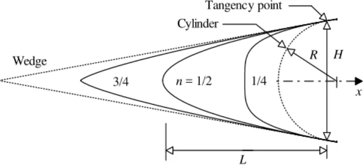
The power-law shapes are modeled by assuming a sharp leading edge of half angle θ with a circular cylinder of radius R inscribed tangent to this wedge. The power law shapes, inscribed between the wedge and the cylinder, are also tangent to the wedge and the circular cylinder at the same common point where they have the same slope angle. The circular cylinder diameter provides a reference for the amount of blunting desired on the leading edge. It is assumed that the wedge half angle is 10 deg, the circular cylinder diameter of 10-2m and power law exponents of 1/4, 1/2 and 3/4, which yield infinite, finite and zero, respectively, for the radius of curvature. Figure 1 illustrates schematically this construction for this set of power law leading edges.
Wedge
Cylinder
n = 1/2 1/4 3/4
L
R H
x
Tangency point
Figure 1. Drawing illustrating the leading edge geometry.
From geometric considerations, the power law constant A is obtained by matching slope on the wedge, circular cylinder and power law body at the tangency point. The common body height H at the tangency point is equal to 2Rcosθ. In this way, for the power law shapes to be investigated in this work, the power law constant A and the body length L from the nose to the tangency point are listed in Table 1.
Table 1. Characteristics of the power law shapes.
Exponent n A(m1-n) L(m) L/H
1/4 1.7034 x 10⁻² 7.8496 x 10⁻³ 0.774
1/2 4.1671 x 10⁻² 1.3963 x 10⁻² 1.418
3/4 8.9438 x 10⁻² 2.0944 x 10⁻² 2.127
A geometrically blunt body is defined to be one with a slope (dy/dx = ∞) at the tip that corresponds to an angle of 90 deg. On the other hand, a geometrically sharp body is defined to be one with a finite slope (dy/dx≠ ∞) at the tip, and the leading-edge radius is zero. The body slope angles at the nose (x = 0) for power law shapes are 90 deg for values of 0 < n < 1. Moreover, the radius of curvature changes from zero to infinity at the same range of n. Therefore, the power law shapes are blunt even though some of them have a zero nose radius. As a result, some power law shapes exhibit both blunt and sharp geometric properties.
Computational Method and Procedure
A number of significant problems in fluid mechanics involve transitional flows, i.e., flows for which the mean free path is of the same order of magnitude as a characteristic dimension of the problem. The most successful numerical technique for modeling complex transitional flows has been the Direct Simulation Monte Carlo (DSMC) method. The fundamental work on DSMC method has been described in the well-known book by Bird (1994). In a review on DSMC methodologies, Bird (1998) has discussed the recent advances of the DSMC method and examined its range of validity. Ivanov and Gimelshein (2002) discuss the current challenges of the DSMC method and examine the issues related to the efficiency and accuracy of the method in the near continuum regime, as well as its use for modeling of rarefied flows with real gas effects.
simulation time of the DSMC method is a real physical time and all DSMC calculations are treated as unsteady state. The solution of the steady-state case is the asymptotic limit of the unsteady flow.
In this study, the molecular collisions are modeled using the variable hard sphere (VHS) molecular model (Bird, 1981). In this model, the temperature dependency of the viscosity is considered by a variable cross section that is inversely proportional to the relative collision energy between the colliding molecules. The energy exchange between kinetic and internal modes is controlled by Borgnakke-Larsen statistical model (Borgnakke and Larsen, 1975). The essential feature of this model is that a part of collisions is treated as completely inelastic, and the reminder of the molecular collisions is regarded as elastic. Simulations are performed using air as working fluid with two chemical species, N2 and O2. Energy exchanges between the translational and internal modes are considered. The vibrational temperature is controlled by the distribution of energy between the translational and rotational modes after an inelastic collision. The probability of an inelastic collision determines the rate at which energy is transferred between the translational and internal modes after an inelastic collision. For a given collision, the probabilities are designated by the inverse of the relaxation numbers, which correspond to the number of collisions necessary, on average, for a molecule to relax. The relaxation numbers are traditionally given as constants, 5 for rotation and 50 for vibration. Diffuse reflection with full thermal accommodation is assumed for the gas-surface interaction modeling. In this model, the reflection of the impinging molecules is not related to the pre-impingement state of the molecules.
The physical space is divided into a certain number of regions, which are subdivided into computational cells. The dimensions of the cells must be such that the change in flow properties across each cell is small compared to the mean free path. The cell provides a convenient reference for the sampling of the macroscopic gas properties. The smallest unit of physical space is the subcell, where the collision partners are selected for the establishment of the collision rate. Time is advanced in discrete steps such that each step is small in comparison with the mean collision time, which is defined as the mean time between the successive collisions suffered by any particular molecule. More details for estimating the computational requirements of DSMC simulations are presented at length by Rieffel (1999).
x
L y
η
ξ v
u
θ H/2
Outer c om putational boundary
Regions
Body s hape
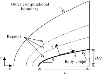
Figure 2. Schematic view of the computational domain.
The computational domain is made large enough so that the upstream and side boundaries can be specified as freestream conditions. A view of the computational domain is depicted in Fig. 2. Only half of the body needs to be considered because of its
symmetry. The flow at the downstream outflow boundary is predominantly supersonic and vacuum conditions are specified (Bird, 1994).
Numerical accuracy in DSMC method depends on the grid resolution chosen as well as the number of particles per computational cell. Both effects were investigated to determine the number of cells and the number of particles required to achieve grid independence solutions for the thermal nonequilibrium flow that arises near the leading edges. A discussion of both effects on the aerodynamic surface quantities is described in the appendix.
The freestream conditions used in the present calculations are those given by Santos (2001). Table 2 and Table 3 summarized the freesteam conditions and the gas properties (Bird, 1994), respectively. The freestream velocity V∞ is assumed to be constant at 2.9 km/s, which corresponds to freestream Mach number M∞ of 10. The wall temperature Tw is assumed constant at 880 K, chosen to be four times the freestream temperature.
The overall Knudsen number is defined as the ratio of the molecular mean free path in the freestream gas to a characteristic dimension of the flowfield. In the present study, the characteristic dimension was defined as being the diameter of the circular cylinder (see Fig. 1). Therefore, the freestream Knudsen number corresponds to Kn∞ (= λ∞/2R) of 0.0903. Finally, the freestream Reynolds number by unit meter Re∞ is 17889.
Table 2. Freestream conditions.
Parameter Value Unit
Velocity (V∞) 2900 m/s
Temperature (T∞) 220.0 K
Pressure (p∞) 5.582 N/m2
Density (ρ∞) 8.753 x 10⁻⁵ kg/m3 Viscosity (µ∞) 1.455 x 10⁻⁵ Ns/m2 Number density (n∞) 1.821 x 10²¹ m-3
Mean free path (λ∞) 9.03 x 10⁻⁴ m
Table 3. Gas properties.
Parameter O2 N2 Unit
Molecular mass (m) 5.312 x 10⁻²⁶ 4.650 x 10⁻²⁶ kg Molecular diameter (d) 4.010 x 10⁻¹⁰ 4.110 x 10⁻¹⁰ m
Mole fraction (X) 0.237 0.763
Viscosity index (ω) 0.77 0.74
Computational Results and Discussion
Attention is now focused on the heat transfer calculations and on the drag coefficient obtained from the DSMC results. The simulations were performed, as mentioned above, for power law exponents of 1/4, 1/2, and 3/4. The present calculations correspond to freestream Mach number of 10, wall temperature of 880 K, and freestream conditions associated to an altitude of 70 km.
The heat transfer coefficient Ch is defined as being,
3 2 1 ∞ ∞
=
V q
Ch w
ρ (4)
∑
⎪ ⎪ ⎭ ⎪ ⎪ ⎬ ⎫
⎪ ⎪ ⎩ ⎪ ⎪ ⎨ ⎧
⎥⎦ ⎤ ⎢⎣
⎡ + +
+ ⎥⎦ ⎤ ⎢⎣
⎡ + +
= + =
=
N
j
r Vj Rj j j
i Vj Rj j j
r i w
e e c m
e e c m
q q q
1 2
2
2 1 2 1
(5)
where N is the number of molecules colliding with the surface by unit time and unit area, m is the mass of the molecules, c is the thermal velocity of the molecules, eR and eV stand for the rotational and vibrational energies, and subscripts i and r refer to incident and reflected molecules.
The heat flux qw is based upon the gas-surface interaction model of fully accommodated, completely diffuse re-emission. This is the most common model assumed, even though it is well known that some degree of specular reflection and less than complete accommodation are more realistic assumptions (Gilmore and Harvey, 1994).
0.0 0.2 0.4 0.6 0.8
0.0001 0.001 0.01 0.1 1 10 30
C
h
= 3/4 = 1/2 = 1/4 n
n
n
s/λ∞
Figure 3. Heat transfer coefficient as a function of the arc length for power law exponents of 1/4, 1/2 and 3/4.
0.0 0.2 0.4 0.6 0.8 1.0
90 80 70 60 50 40 30 20 10
C
h
FM = 3/4 = 1/2 = 1/4
θ (degree)
n
n
n
Figure 4. Heat transfer coefficient as a function of the body slope angle for power law exponents of 1/4, 1/2 and 3/4.
0.0 1.0 2.0 3.0
0.0 4.0 8.0 12.0 16.0 20.0
K(n)
= 1/4
= 1/2
= 3/4
s/λ∞
n
n
n
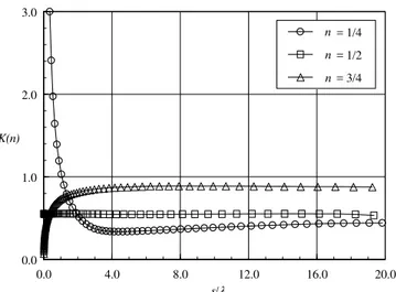
Figure 5. Distribution of K(n) as a function of the arc length for power law exponents of 1/4, 1/2 and 3/4.
0.0 1.0 2.0 3.0
0.001 0.01 0.1 1 10 20
K(n)
= 1/4
= 1/2
= 3/4
s/λ∞ n
n
n
Figure 6. Distribution of K(n) in the vicinity of the stagnation as a function of the arc length for power law exponents of 1/4, 1/2 and 3/4.
The effect of the power law exponent on the heat transfer coefficient Ch is illustrated in Fig. 3 as a function of the dimensionless arc length s/λ∞, measured from the stagnation point. It is seen that the heat transfer coefficient is sensitive to the power law exponent n near the stagnation point. It presents the maximum value in the stagnation point and drops off a short distance away of the leading edge as the power law exponent increases. Also, it is seen that the blunter the leading edge is the lower the heat transfer coefficient in the stagnation region.
The leading edge geometry effect can also be seen by comparing the computational results with that predicted by considering free molecular (FM) flow (Bird, 1994). Figure 4 displays this comparison for the heat transfer coefficient as a function of the body slope angle θ. These curves indicate that the heat transfer coefficient Ch increases as the leading edge becomes sharp, and approaches the free molecular value for the conditions investigated in this work.
even though the radius of curvature goes to zero for the n = 3/4 case, and goes to infinity for the n = 1/4 case.
In order to verify the dependence of the heat transfer coefficient Ch on the leading edge radius of curvature, the product Ch√(Rc/λ∞), named here by function K(n), is obtained from the DSMC results for the power law shapes investigated. Hence, Ch√(Rc/λ∞) represents the dimensionless form of Eq. (1). Figures 5 (linear scaling) and 6 (log scaling) demonstrate this product as a function of the dimensionless arc length along the body surface. Interesting features can be drawn from Figs. 5 and 6. In the vicinity of the stagnation point, the dependence of the heat transfer coefficient on the radius of curvature follows that predicted by the continuum flow, Eq. (1), for the power law shape with finite radius, n = 1/2 case. As would be expected, the dependence of the heat transfer coefficient on the radius of curvature in the stagnation region does not hold for power law leading edges defined by cases with n≠ 1/2. Moreover, the function K(n) surprising reaches a constant value downstream to the stagnation region for the cases investigated. The constant value, which is a function of the power law exponent, is reached faster for the n = 3/4 than for the n = 1/4 case. As a result, it is seen that the heat transfer to the body is inversely proportional to the square root of the curvature radius of the power law shapes far from the stagnation region, independently of the power law exponent for the range 1/4 < n < 3/4.
Referring to Figs. 5 and 6, at first glance, one could conclude that power law shape defined by n = 3/4 gives lower value for heat flux at the stagnation point than n = 1/2 shape. Unfortunately, this does not hold as is demonstrated in Fig. 3.
The drag on a surface in a gas flow results from the interchange of momentum between the surface and the molecules colliding with the surface. The total drag is obtained by the integration of the pressure and shear stress distributions from the nose of the leading edge to the station L, which corresponds to the tangent point common to all of the body shapes (see Fig. 1). It is important to mention that the values for the total drag presented in this section were obtained by assuming the shapes acting as leading edges. Therefore, no base pressure effects were taken into account in the calculations. Results are normalized by ½ρ∞V∞2H and presented as total drag coefficient Cd and its components of pressure drag coefficient and skin friction drag coefficient.
0.25 0.5 0.75
0.0 0.3 0.6 0.9 1.2 1.5
C
d
Power law exponent n C
fd Cpd Cd
Figure 7. Pressure drag, skin friction drag and total drag coefficient as a function of the power law exponent n.
0 20 40 60 80 100
0.25 0.50 0.75
Power law exponent n Pressure drag Skin friction drag
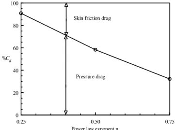
%Cd
Figure 8. Pressure and skin friction drag contributions on the total drag as a function of the power law exponent n.
Figure 7 illustrates the total drag coefficient as a function of the power law exponent n. The contributions of the pressure drag coefficient and the skin friction coefficient are also displayed in this figure. For n = 1/4 case, the total drag coefficient is dominated by pressure drag, a characteristic of a blunt body. In contrast, for n = 3/4, the total drag coefficient is dominated by the skin friction drag, a characteristic of a sharp body. As the net effect on total drag depends on these opposite behaviors, appreciable changes are observed in the total drag coefficient for the power law exponent range investigated. As a reference, the total drag coefficient for the n = 1/4 case is around 24% higher than that for the n = 3/4 case.
Figure 8 displays the percentage of the skin friction drag and pressure drag on total drag. It is seen that for power law exponent of 1/4, the shear forces account for only 9% of the total drag forces on the leading edge, whereas for power law exponent of 3/4, it accounts for
68%.
Concluding Remarks
Through the use of DSMC method, the heat flux to and drag acting on power law shapes have been investigated. The calculations provided information concerning the nature of the heat transfer coefficient and the total drag coefficient along the body surface resulting from variations in the body shape for the idealized situation of two-dimensional hypersonic rarefied flow. Results for power law exponents of 1/4, 1/2, and 3/4 indicate that the heat flux approaches that one predicted by the free molecular flow as the power law shape becomes aerodynamically sharp, for the flow conditions considered. A substantial reduction of the aerodynamic heating at the stagnation point is observed as the power law exponent decreases. On the other hand, a power law exponent decrease is associated with a drag increase. Furthermore, the stagnation point heating for the power law shapes does not follow that one for classical blunt body in the vicinity of the leading edge for power law exponents different from 1/2. Nevertheless, the heat transfer varies inversely with the square root of the radius of curvature far from the stagnation region.
Appendix
interest for the present study since insufficient grid resolution can reduce significantly the accuracy of the predicted aerodynamic heating and forces acting on the body surface. Hence, heat transfer, pressure and skin friction coefficients were used as the representative parameters for the grid sensitivity study. However, because of the reduced number of pages in the paper, the analysis will be shown only for heat transfer coefficient related to the n = 1/2 case.
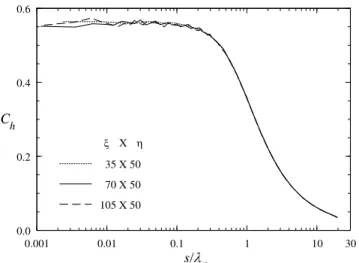
The effect of altering the size of the computational cells is investigated for a series of three simulations with grids of 35 (coarse), 70 (standard) and 105 (fine) cells in the ξ-direction and 50 cells in the η-direction (see Fig. 2). Each grid was made up of nonuniform cell spacing in both directions. The effect of changing the number of cells in the ξ-direction is illustrated in Fig. A1 as it impacts the calculated heat transfer coefficient. The comparison shows that the calculated results are rather insensitive to the range of cell spacing considered.
In analogous fashion, an examination was made in the η-direction. The sensitivity of the calculated results to cell size variations in the η-direction is displayed in Fig. A2 for heat transfer coefficient. In this figure, a new series of three simulations with grid of 70 cells in the ξ-direction and 25 (coarse), 50 (standard) and 75 (fine) cells in the η-direction is compared. The cell spacing in both directions is again nonuniform. According to Fig. A2, the results for the three grids are approximately the same, indicating that the standard grid, 70 X 50 cells, is essentially grid independent. For the standard case, the cell size in the η-direction is always less than the local mean free path length in the vicinity of the surface.
A similar examination was made for the number of molecules. The sensitivity of the calculated results to number of molecule variations is demonstrated in Fig. A3 for heat transfer coefficient. The standard grid, 70 x 50 cells, corresponds to a total of 112,300 molecules. Two new cases using the same grid were investigated. These new cases correspond to, on average, 63,600 and 170,300 molecules in the entire computational domain. It is seen that the standard grid with a total of 112,300 molecules is enough for the computation of the aerodynamic surface quantities.
s/λ∞
s/λ∞
0.0 0.2 0.4 0.6
0.0 0.2 0.4 0.6
0.001 0.01 0.1 1 10 30
0.001 0.01 0.1 1 10 30
Ch
35 X 50
70 X 50
105 X 50
ξ X η
Figure A1. Effect of altering the cell size in the ξ-direction on heat transfer coefficient.
s/λ∞
s/λ∞
0.0 0.2 0.4 0.6
0.0 0.2 0.4 0.6
0.001 0.01 0.1 1 10 30
0.001 0.01 0.1 1 10 30
Ch
70 X 25
70 X 50
70 X 75
ξ X η
Figure A2. Effect of altering the cell size in the η-direction on heat transfer coefficient.
s/
λ
∞0.0 0.2 0.4 0.6
0.0 0.2 0.4 0.6
0.001 0.01 0.1 1 10 30
0.001 0.01 0.1 1 10 30
Ch
63,600 Mols.
112,300 Mols.
170,300 Mols.
Figure A3. Effect of altering the number of molecules on heat transfer coefficient.
References
Bird, G. A., 1981, “Monte Carlo Simulation in an Engineering Context”, Progress in Astronautics and Aeronautics: Rarefied gas Dynamics, ed. by Sam S. Fisher, AIAA New York, Vol. 74, part I, pp.239-255.
Bird, G. A., 1994, “Molecular Gas Dynamics and the Direct Simulation of Gas Flows”, 1st edition, Oxford University Press, Oxford, England, UK., 458p.
Bird, G. A., 1998, “Recent Advances and Current Challenges for DSMC”, Computers Math. Applic., Vol. 35, pp. 1-14.
Borgnakke, C., and Larsen, P. S., 1975, “Statistical Collision Model for Monte Carlo Simulation of Polyatomic Gas Mixture”, J of computational Physics, Vol. 18, pp.405-420.
Cohen, N. B., 1961, “Boundary-Layer Similar Solutions and Correlation Equations for Laminar Heat-Transfer Distribution in Equilibrium Air at Velocities up to 41,000 feet per second”, NASA TR R-118.
DeJarnette, F. R., Hamilton, H. H., Weilmuenster, K. J., and Cheatwood, F. M., 1987, “A Review of some Approximate Methods Used in Aerodynamic Heating Analysis”, J. of Thermophysics and Heat Transfer, Vol. 1, pp. 5-12.
Fay, J. A., and Riddell, F. R., 1958, “Theory of Stagnation Point Heat Transfer in Dissociated Air”, J. of Aeronautical Sciences, Vol. 25, pp. 73-85.
Haas, B. L., and Fallavollita, M. A., 1994, “Flow Resolution and Domain Influence in Rarefied Hypersonic Blunt-Body Flows”, J. of Thermophysics and Heat Transfer, Vol. 8, pp.751-757.
Ivanov, M. S. and Gimelshein, S. F. 2002, “Current Status and Prospects of the DSMC Modeling of Near-Continuum Flows of Non-Reacting and Reacting Gases”, Rarefied Gas Dynamics, 23rd International Symposium, Whistler, BC, Canada, Eds. A. D. Ketsdever and E. P. Muntz, pp. 339-348.
Lees, L., 1956, “Laminar Heat Transfer over Blunt-Nosed Bodies at Hypersonic Flight Speeds”, Jet Propulsion, Vol. 26, pp. 259-269.
Mason, W. H., and Lee, J., 1994, “Aerodynamically Blunt and Sharp Bodies”, J. of Spacecraft and Rockets, Vol. 31, pp.378-382.
Rieffel, M. A., 1999, “A Method for Estimating the Computational Requirements of DSMC Simulations”, J. of Computational Physics, Vol. 149, pp. 95-113.
Romig, M., 1956, “Stagnation Point Heat Transfer for Hypersonic Flow”, Jet Propulsion, Vol. 26, pp. 1098-1101.
Santos, W. F. N., 2001, “Direct Simulation Monte Carlo of Rarefied hypersonic Flow on Power Law Shaped Leading Edges”, Ph.D. Thesis, University of Maryland, College Park, MD, USA, 324p.
Sibulkin, M., 1952, “Heat Transfer Near the Forward Stagnation Point of a Body of Revolution”, J. of Aeronautical Sciences, Vol. 19 pp. 570-571.
Sutton, K., and Graves, R. A. Jr, 1971, “A General Stagnation-Point Convective-Heating Equation for Arbitrary Gas Mixtures”, NASA TR R-376.
Zoby, E. V., Moss, N. J., and Sutton, K., 1981, “Approximate Convective-Heating Equations for Hypersonic Flows”, J. of Spacecraft and Rockets, Vol. 18, pp.64-70.